The Safer Affordable Fuel-Efficient (SAFE) Vehicles Rule for Model Years 2021-2026 Passenger Cars and Light Trucks, 42986-43500 [2018-16820]

Download as PDF 42986 Federal Register / Vol. 83, No. 165 / Friday, August 24, 2018 / Proposed Rules DEPARTMENT OF TRANSPORTATION National Highway Traffic Safety Administration 49 CFR Parts 523, 531, 533, 536, and 537 ENVIRONMENTAL PROTECTION AGENCY 40 CFR Parts 85 and 86 [NHTSA–2018–0067; EPA–HQ–OAR–2018– 0283; FRL–9981–74–OAR] RIN 2127–AL76; RIN 2060–AU09 The Safer Affordable Fuel-Efficient (SAFE) Vehicles Rule for Model Years 2021–2026 Passenger Cars and Light Trucks Environmental Protection Agency and National Highway Traffic Safety Administration. ACTION: Notice of proposed rulemaking. AGENCY: The National Highway Traffic Safety Administration (NHTSA) and the Environmental Protection Agency (EPA) are proposing the ‘‘Safer Affordable Fuel-Efficient (SAFE) Vehicles Rule for Model Years 2021–2026 Passenger Cars and Light Trucks’’ (SAFE Vehicles Rule). The SAFE Vehicles Rule, if finalized, would amend certain existing Corporate Average Fuel Economy (CAFE) and tailpipe carbon dioxide emissions standards for passenger cars and light trucks and establish new standards, all covering model years 2021 through 2026. More specifically, NHTSA is proposing new CAFE standards for model years 2022 through 2026 and amending its 2021 model year CAFE standards because they are no longer maximum feasible standards, and EPA is proposing to amend its carbon dioxide emissions standards for model years 2021 through 2025 because they are no longer appropriate and reasonable in addition to establishing new standards for model year 2026. The preferred alternative is to retain the model year 2020 standards (specifically, the footprint target curves for passenger cars and light trucks) for both programs through model year 2026, but comment is sought on a range of alternatives discussed throughout this document. Compared to maintaining the post-2020 standards set forth in 2012, current estimates indicate that the proposed SAFE Vehicles Rule would save over 500 billion dollars in societal costs and reduce highway fatalities by 12,700 lives (over the lifetimes of vehicles through MY 2029). U.S. fuel consumption would increase by about sradovich on DSK3GMQ082PROD with PROPOSALS2 SUMMARY: VerDate Sep<11>2014 23:42 Aug 23, 2018 Jkt 244001 half a million barrels per day (2–3 percent of total daily consumption, according to the Energy Information Administration) and would impact the global climate by 3/1000th of one degree Celsius by 2100, also when compared to the standards set forth in 2012. DATES: Comments: Comments are requested on or before October 23, 2018. Under the Paperwork Reduction Act, comments on the information collection provisions must be received by the Office of Management and Budget (OMB) on or before October 23, 2018. See the SUPPLEMENTARY INFORMATION section on ‘‘Public Participation,’’ below, for more information about written comments. Public Hearings: NHTSA and EPA will jointly hold three public hearings in Washington, DC; the Detroit, MI area; and in the Los Angeles, CA area. The agencies will announce the specific dates and addresses for each hearing location in a supplemental Federal Register notice. The agencies will accept oral and written comments to the rulemaking documents, and NHTSA will also accept comments to the Draft Environmental Impact Statement (DEIS) at these hearings. The hearings will start at 10 a.m. local time and continue until everyone has had a chance to speak. See the SUPPLEMENTARY INFORMATION section on ‘‘Public Participation,’’ below, for more information about the public hearings. You may send comments, identified by Docket No. EPA–HQ– OAR–2018–0283 and/or NHTSA–2018– 0067, by any of the following methods: • Federal eRulemaking Portal: https:// www.regulations.gov. Follow the instructions for sending comments. • Fax: EPA: (202) 566–9744; NHTSA: (202) 493–2251. • Mail: Æ EPA: Environmental Protection Agency, EPA Docket Center (EPA/DC), Air and Radiation Docket, Mail Code 28221T, 1200 Pennsylvania Avenue NW, Washington, DC 20460, Attention Docket ID No. EPA–HQ–OAR–2018– 0283. In addition, please mail a copy of your comments on the information collection provisions for the EPA proposal to the Office of Information and Regulatory Affairs, Office of Management and Budget (OMB), Attn: Desk Officer for EPA, 725 17th St. NW, Washington, DC 20503. Æ NHTSA: Docket Management Facility, M–30, U.S. Department of Transportation, West Building, Ground Floor, Rm. W12–140, 1200 New Jersey Avenue SE, Washington, DC 20590. • Hand Delivery: ADDRESSES: PO 00000 Frm 00002 Fmt 4701 Sfmt 4702 Æ EPA: Docket Center (EPA/DC), EPA West, Room B102, 1301 Constitution Avenue NW, Washington, DC, Attention Docket ID No. EPA–HQ–OAR–2018– 0283. Such deliveries are only accepted during the Docket’s normal hours of operation, and special arrangements should be made for deliveries of boxed information. Æ NHTSA: West Building, Ground Floor, Rm. W12–140, 1200 New Jersey Avenue SE, Washington, DC 20590, between 9 a.m. and 4 p.m. Eastern Time, Monday through Friday, except Federal holidays. Instructions: All submissions received must include the agency name and docket number or Regulatory Information Number (RIN) for this rulemaking. All comments received will be posted without change to https:// www.regulations.gov, including any personal information provided. For detailed instructions on sending comments and additional information on the rulemaking process, see the ‘‘Public Participation’’ heading of the SUPPLEMENTARY INFORMATION section of this document. Docket: For access to the dockets to read background documents or comments received, go to https:// www.regulations.gov, and/or: • For EPA: EPA Docket Center (EPA/ DC), EPA West, Room 3334, 1301 Constitution Avenue NW, Washington, DC 20460. The Public Reading Room is open from 8:30 a.m. to 4:30 p.m., Monday through Friday, excluding legal holidays. The telephone number for the Public Reading Room is (202) 566–1744. • For NHTSA: Docket Management Facility, M–30, U.S. Department of Transportation, West Building, Ground Floor, Rm. W12–140, 1200 New Jersey Avenue SE, Washington, DC 20590. The Docket Management Facility is open between 9 a.m. and 4 p.m. Eastern Time, Monday through Friday, except Federal holidays. FOR FURTHER INFORMATION CONTACT: EPA: Christopher Lieske, Office of Transportation and Air Quality, Assessment and Standards Division, Environmental Protection Agency, 2000 Traverwood Drive, Ann Arbor, MI 48105; telephone number: (734) 214– 4584; fax number: (734) 214–4816; email address: lieske.christopher@ epa.gov, or contact the Assessment and Standards Division, email address: otaqpublicweb@epa.gov. NHTSA: James Tamm, Office of Rulemaking, Fuel Economy Division, National Highway Traffic Safety Administration, 1200 New Jersey Avenue SE, Washington, DC 20590; telephone number: (202) 493– 0515. E:\FR\FM\24AUP2.SGM 24AUP2 Federal Register / Vol. 83, No. 165 / Friday, August 24, 2018 / Proposed Rules SUPPLEMENTARY INFORMATION: I. Overview of Joint NHTSA/EPA Proposal II. Technical Foundation for NPRM Analysis III. Proposed CAFE and CO2 Standards for MYs 2021–2026 IV. Alternative CAFE and GHG Standards Considered for MYs 2021/22–2026 V. Proposed Standards, the Agencies’ Statutory Obligations, and Why the Agencies Propose To Choose Them Over the Alternatives VI. Preemption of State and Local Laws VII. Impacts of the Proposed CAFE and CO2 Standards VIII. Impacts of Alternative CAFE and CO2 Standards Considered for MYs 2021/22– 2026 IX. Vehicle Classification X. Compliance and Enforcement XI. Public Participation XII. Regulatory Notices and Analyses I. Overview of Joint NHTSA/EPA Proposal sradovich on DSK3GMQ082PROD with PROPOSALS2 A. Executive Summary In this notice, the National Highway Traffic Safety Administration (NHTSA) and the Environmental Protection Agency (EPA) (collectively, ‘‘the agencies’’) are proposing the ‘‘Safer Affordable Fuel-Efficient (SAFE) Vehicles Rule for Model Years 2021– 2026 Passenger Cars and Light Trucks’’ (SAFE Vehicles Rule). The proposed SAFE Vehicles Rule would set Corporate Average Fuel Economy (CAFE) and carbon dioxide (CO2) emissions standards, respectively, for passenger cars and light trucks manufactured for sale in the United States in model years (MYs) 2021 through 2026.1 CAFE and CO2 standards have the power to transform the vehicle fleet and affect Americans’ lives in significant, if not always immediately obvious, ways. The proposed SAFE Vehicles Rule seeks to ensure that government action on these standards is appropriate, reasonable, consistent with law, consistent with current and foreseeable future economic realities, and supported by a transparent assessment of current facts and data. The agencies must act to propose and finalize these standards and do not have discretion to decline to regulate. Congress requires NHTSA to set CAFE standards for each model year.2 Congress also requires EPA to set emissions standards for light-duty vehicles if EPA has made an ‘‘endangerment finding’’ that the pollutant in question—in this case, 1 NHTSA sets CAFE standards under the Energy Policy and Conservation Act of 1975 (EPCA), as amended by the Energy Independence and Security Act of 2007 (EISA). EPA sets CO2 standards under the Clean Air Act (CAA). 2 49 U.S.C. 32902. VerDate Sep<11>2014 23:42 Aug 23, 2018 Jkt 244001 CO2—‘‘cause[s] or contribute[s] to air pollution which may reasonably be anticipated to endanger public health or welfare.’’ 3 NHTSA and EPA are proposing these standards concurrently because tailpipe CO2 emissions standards are directly and inherently related to fuel economy standards,4 and if finalized, these rules would apply concurrently to the same fleet of vehicles. By working together to develop these proposals, the agencies reduce regulatory burden on industry and improve administrative efficiency. Consistent with both agencies’ statutes, this proposal is entirely de novo, based on an entirely new analysis reflecting the best and most up-to-date information available to the agencies at the time of this rulemaking. The agencies worked together in 2012 to develop CAFE and CO2 standards for MYs 2017 and beyond; in that rulemaking action, EPA set CO2 standards for MYs 2017–2025, while NHTSA set final CAFE standards for MYs 2017–2021 and also put forth ‘‘augural’’ CAFE standards for MYs 2022–2025, consistent with EPA’s CO2 standards for those model years. EPA’s CO2 standards for MYs 2022–2025 were subject to a ‘‘mid-term evaluation,’’ by which EPA bound itself through regulation to re-evaluate the CO2 standards for those model years and to undertake to develop new CO2 standards through a regulatory process if it concluded that the previously finalized standards were no longer appropriate. EPA regulations on the mid-term evaluation process required EPA to issue a Final Determination no later than April 1, 2018 on whether the GHG standards for MY 2022–2025 lightduty vehicles remain appropriate under 3 42 U.S.C. 7521, see also 74 FR 66495 (Dec. 15, 2009) (‘‘Endangerment and Cause or Contribute Findings for Greenhouse Gases under Section 202(a) of the Clean Air Act’’). 4 See, e.g., 75 FR 25324, at 25327 (May 7, 2010) (‘‘The National Program is both needed and possible because the relationship between improving fuel economy and reducing tailpipe CO2 emissions is a very direct and close one. The amount of those CO2 emissions is essentially constant per gallon combusted of a given type of fuel. Thus, the more fuel efficient a vehicle is, the less fuel it burns to travel a given distance. The less fuel it burns, the less CO2 it emits in traveling that distance. [citation omitted] While there are emission control technologies that reduce the pollutants (e.g., carbon monoxide) produced by imperfect combustion of fuel by capturing or converting them to other compounds, there is no such technology for CO2. Further, while some of those pollutants can also be reduced by achieving a more complete combustion of fuel, doing so only increases the tailpipe emissions of CO2. Thus, there is a single pool of technologies for addressing these twin problems, i.e., those that reduce fuel consumption and thereby reduce CO2 emissions as well.’’) PO 00000 Frm 00003 Fmt 4701 Sfmt 4702 42987 section 202(a) of the Clean Air Act.5 The regulations also required the issuance of a draft Technical Assessment Report (TAR) by November 15, 2017, an opportunity for public comment on the draft TAR, and, before making a Final Determination, an opportunity for public comment on whether the GHG standards for MY 2022–2025 remain appropriate. In July 2016, the draft TAR was issued for public comment jointly by the EPA, NHTSA, and the California Air Resources Board (CARB).6 Following the draft TAR, EPA published a Proposed Determination for public comment on December 6, 2016 and provided less than 30 days for public comments over major holidays.7 EPA published the January 2017 Determination on EPA’s website and regulations.gov finding that the MY 2022–2025 standards remained appropriate.8 On March 15, 2017, President Trump announced a restoration of the original mid-term review timeline. The President made clear in his remarks, ‘‘[i]f the standards threatened auto jobs, then commonsense changes’’ would be made in order to protect the economic viability of the U.S. automotive industry.’’ 9 In response to the President’s direction, EPA announced in a March 22, 2017, Federal Register notice, its intention to reconsider the Final Determination of the mid-term evaluation of GHGs emissions standards for MY 2022–2025 light-duty vehicles.10 The Administrator stated that EPA would coordinate its reconsideration with the rulemaking process to be undertaken by NHTSA regarding CAFE standards for cars and light trucks for the same model years. On August 21, 2017, EPA published a notice in the Federal Register announcing the opening of a 45-day public comment period and inviting stakeholders to submit any additional comments, data, and information they believed were relevant to the Administrator’s reconsideration of the 5 40 CFR 86.1818–12(h)(1); see also 77 FR 62624 (Oct. 15, 2012). 6 81 FR 49217 (Jul. 27, 2016). 7 81 FR 87927 (Dec. 6, 2016). 8 Docket item EPA–HQ–OAR–2015–0827–6270 (EPA–420–R–17–001). This conclusion generated a significant amount of public concern. See, e.g., Letter from Auto Alliance to Scott Pruitt, Administrator, Environmental Protection Agency (Feb. 21, 2017); Letter from Global Automakers to Scott Pruitt, Administrator, Environmental Protection Agency (Feb. 21, 2017). 9 See https://www.whitehouse.gov/briefingsstatements/remarks-president-trump-americancenter-mobility-detroit-mi/. 10 82 FR 14671 (Mar. 22, 2017). E:\FR\FM\24AUP2.SGM 24AUP2 42988 Federal Register / Vol. 83, No. 165 / Friday, August 24, 2018 / Proposed Rules January 2017 Determination.11 EPA held a public hearing in Washington DC on September 6, 2017.12 EPA received more than 290,000 comments in response to the August 21, 2017 notice.13 EPA has since concluded, based on more recent information, that those standards are no longer appropriate.14 NHTSA’s ‘‘augural’’ CAFE standards for MYs 2022–2025 were not final in 2012 because Congress prohibits NHTSA from finalizing new CAFE standards for more than five model years in a single rulemaking.15 NHTSA was therefore obligated from the beginning to undertake a new rulemaking to set CAFE standards for MYs 2022–2025. The proposed SAFE Vehicles Rule begins the rulemaking process for both agencies to establish new standards for MYs 2022–2025 passenger cars and light trucks. Standards are concurrently being proposed for MY 2026 in order to provide regulatory stability for as many years as is legally permissible for both agencies together. Separately, the proposed SAFE Vehicles Rule includes revised standards for MY 2021 passenger cars and light trucks. The information now available and the current analysis 11 82 FR 39551 (Aug. 21, 2017). FR 39976 (Aug. 23, 2017). 13 The public comments, public hearing transcript, and other information relevant to the Mid-term Evaluation are available in docket EPA– HQ–OAR–2015–0827. 14 83 FR 16077 (Apr. 2, 2018). 15 49 U.S.C. 32902. sradovich on DSK3GMQ082PROD with PROPOSALS2 12 82 VerDate Sep<11>2014 23:42 Aug 23, 2018 Jkt 244001 suggest that the CAFE standards previously set for MY 2021 are no longer maximum feasible, and the CO2 standards previously set for MY 2021 are no longer appropriate. Agencies always have authority under the Administrative Procedure Act to revisit previous decisions in light of new facts, as long as they provide notice and an opportunity for comment, and it is plainly the best practice to do so when changed circumstances so warrant.16 Thus, the proposed SAFE Vehicles Rule would maintain the CAFE and CO2 standards applicable in MY 2020 for MYs 2021–2026, while taking comment on a wide range of alternatives, including different stringencies and retaining existing CO2 standards and the augural CAFE standards.17 Table I–4 16 See FCC v. Fox Television, 556 U.S. 502 (2009). This does not mean that the miles per gallon and grams per mile levels that were estimated for the MY 2020 fleet in 2012 would be the ‘‘standards’’ going forward into MYs 2021–2026. Both NHTSA and EPA set CAFE and CO2 standards, respectively, as mathematical functions based on vehicle footprint. These mathematical functions that are the actual standards are defined as ‘‘curves’’ that are separate for passenger cars and light trucks, under which each vehicle manufacturer’s compliance obligation varies depending on the footprints of the cars and trucks that it ultimately produces for sale in a given model year. It is the MY 2020 CAFE and CO2 curves which we propose would continue to apply to the passenger car and light truck fleets for MYs 2021–2026. The mpg and g/mi values which those curves would eventually require of the fleets in those model years would be known for certain only at the ends of each of those model years. While it is convenient to discuss CAFE and CO2 standards as a set ‘‘mpg,’’ ‘‘g/mi,’’ or ‘‘mpg-e’’ number, attempting to define those values today will end up being inaccurate. 17 Note: PO 00000 Frm 00004 Fmt 4701 Sfmt 4702 below presents those alternatives. We note further that prior to MY 2021, CO2 targets include adjustments reflecting the use of automotive refrigerants with reduced global warming potential (GWP) and/or the use of technologies that reduce the refrigerant leaks, and optionally offsets for nitrous oxide and methane emissions. In the interests of harmonizing with the CAFE program, EPA is proposing to exclude air conditioning refrigerants and leakage, and nitrous oxide and methane emissions for compliance with CO2 standards after model year 2020 but seeks comment on whether to retain these element, and reinsert A/C leakage offsets, and remain disharmonized with the CAFE program. EPA also seeks comment on whether to change existing methane and nitrous oxide standards that were finalized in the 2012 rule. Specifically, EPA seeks information from the public on whether those existing standards are appropriate, or whether they should be revised to be less stringent or more stringent based on any updated data. While actual requirements will ultimately vary for automakers depending upon their individual fleet mix of vehicles, many stakeholders will likely be interested in the current estimate of what the MY 2020 CAFE and CO2 curves would translate to, in terms of miles per gallon (mpg) and grams per mile (g/mi), in MYs 2021–2026. These estimates are shown in the following tables. BILLING CODE 4910–59–P E:\FR\FM\24AUP2.SGM 24AUP2 Federal Register / Vol. 83, No. 165 / Friday, August 24, 2018 / Proposed Rules 42989 Table 1-1- Average of OEM' s CAFE an d CO2 E sf 1mat ed R eqmreme nts for Passenger Cars Model Year Avg. ofOEMs' Est. Requirements CAFE (mpg) C02 (g/mi) 2017 2018 2019 2020 2021 2022 2023 2024 2025 2026 39.1 40.5 42.0 43.7 43.7 43.7 43.7 43.7 43.7 43.7 220 210 201 191 204 204 204 204 204 204 Table 1-2- Average of OEM' . d R eqmrem ents for Light Trucks s CAFE an d CO 2 E st1mate Model Year Avg. ofOEMs' Est. Requirements CAFE (mpg) C02 (g/mi) 2017 2018 2019 2020 2021 2022 2023 2024 2025 2026 29.5 30.1 30.6 31.3 31.3 31.3 31.3 31.3 31.3 31.3 294 284 277 269 284 284 284 284 284 284 Table 1-3- Average of OEMs' Estimated CAFE and C02 Requirements (Passenger Cars and Li~ht Trucks) VerDate Sep<11>2014 23:42 Aug 23, 2018 Jkt 244001 PO 00000 34.0 34.9 35.8 36.9 36.9 36.9 36.9 37.0 37.0 37.0 Frm 00005 Fmt 4701 254 244 236 227 241 241 241 241 240 240 Sfmt 4725 E:\FR\FM\24AUP2.SGM EP24AU18.001</GPH> 2017 2018 2019 2020 2021 2022 2023 2024 2025 2026 24AUP2 EP24AU18.000</GPH> sradovich on DSK3GMQ082PROD with PROPOSALS2 Model Year Avg. ofOEMs' Est. Requirements CAFE (mpg) C0 2 (g/mi) 42990 Federal Register / Vol. 83, No. 165 / Friday, August 24, 2018 / Proposed Rules In the tables above, estimated required CO2 increases between MY 2020 and MY 2021 because, again, EPA is proposing to exclude CO2-equivalent emission improvements associated with air conditioning refrigerants and leakage (and, optionally, offsets for nitrous oxide and methane emissions) after model year 2020. As explained above, the agencies are taking comment on a wide range of Ta bl e I- 4 - R egu atory AI ternat1ves c urrently un der c ons1 eratwn Alternative Change in stringency A/C efficiency and offcycle .. provisiOns Baseline/ No-Action MY 2021 standards remain in place; MYs 2022-2025 augural CAFE standards are finalized and GHG standards remain unchanged; MY 2026 standards are set at MY 2025 levels Existing standards through MY 2020, then 0%/year increases for both passenger cars and light trucks, for MY s 2021-2026 Existing standards through MY 2020, then 0.5%/year increases for both passenger cars and light trucks, for MY s 2021-2026 Existing standards through MY 2020, then 0.5%/year increases for both passenger cars and light trucks, for MY s 2021-2026 No change 1 (Proposed) 2 3 4 5 6 7 8 sradovich on DSK3GMQ082PROD with PROPOSALS2 alternatives and have specifically modeled eight alternatives (including the proposed alternative) and the current requirements (i.e., baseline/noaction). The modeled alternatives are provided below: Existing standards through MY 2020, then 1%/year increases for passenger cars and 2%/year increases for light trucks, for MYs 2021-2026 Existing standards through MY 2021, then 1%/year increases for passenger cars and 2%/year increases for light trucks, for MY s 2022-2026 Existing standards through MY 2020, then 2%/year increases for passenger cars and 3 %/year increases for light trucks, for MYs 2021-2026 Existing standards through MY 2020, then 2%/year increases for passenger cars and 3 %/year increases for light trucks, for MYs 2021-2026 Existing standards through MY 2021, then 2%/year increases for passenger cars and 3 %/year increases for light trucks, for MY s 2022-2026 No change No change Phase out these adjustments overMYs 2022-2026 No change C02 Equivalent AC Refrigerant Leakage, Nitrous Oxide and Methane Emissions Included for Compliance? Yes, for all MYs 18 No, beginning 19 in MY 2021 No, beginning in MY 2021 No, beginning in MY 2021 No, beginning in MY 2021 No change No, beginning in MY 2022 No change No, beginning in MY 2021 Phase out these adjustments overMYs 2022-2026 No change No, beginning in MY 2021 No, beginning in MY 2022 Summary of Rationale Since finalizing the agencies’ previous joint rulemaking in 2012 titled ‘‘Final Rule for Model Year 2017 and Later Light-Duty Vehicle Greenhouse Gas Emission and Corporate Average Fuel Economy Standards,’’ and even since EPA’s 2016 and early 2017 ‘‘mid-term evaluation’’ process, the agencies have gathered new information, and have performed new analysis. That new information and analysis has led the 18 Carbon dioxide equivalent of air conditioning refrigerant leakage, nitrous oxide and methane emissions are included for compliance with the EPA standards for all MYs under the baseline/no action alternative. Carbon dioxide equivalent is calculated using the Global Warming Potential (GWP) of each of the emissions. 19 Beginning in MY 2021, the proposal provides that the GWP equivalents of air conditioning refrigerant leakage, nitrous oxide and methane emissions would no longer be able to be included with the tailpipe CO2 for compliance with tailpipe CO2 standards. VerDate Sep<11>2014 23:42 Aug 23, 2018 Jkt 244001 PO 00000 Frm 00006 Fmt 4701 Sfmt 4702 E:\FR\FM\24AUP2.SGM 24AUP2 EP24AU18.002</GPH> BILLING CODE 4910–59–C sradovich on DSK3GMQ082PROD with PROPOSALS2 Federal Register / Vol. 83, No. 165 / Friday, August 24, 2018 / Proposed Rules 42991 agencies to the tentative conclusion that holding standards constant at MY 2020 levels through MY 2026 is maximum feasible, for CAFE purposes, and appropriate, for CO2 purposes. Technologies have played out differently in the fleet from what the agencies assumed in 2012. The technology to improve fuel economy and reduce CO2 emissions has not changed dramatically since prior analyses were conducted: A wide variety of technologies are still available to accomplish the goals of the programs, and a wide variety of technologies would likely be used by industry to accomplish these goals. There remains no single technology that the majority of vehicles made by the majority of manufacturers can implement at low cost without affecting other vehicle attributes that consumers value more than fuel economy and CO2 emissions. Even when used in combination, technologies that can improve fuel economy and reduce CO2 emissions still need to (1) actually work together and (2) be acceptable to consumers and avoid sacrificing other vehicle attributes while also avoiding undue increases in vehicle cost. Optimism about the costs and effectiveness of many individual technologies, as compared to recent prior rounds of rulemaking, is somewhat tempered; a clearer understanding of what technologies are already on vehicles in the fleet and how they are being used, again as compared to recent prior rounds of rulemaking, means that technologies that previously appeared to offer significant ‘‘bang for the buck’’ may no longer do so. Additionally, in light of the reality that vehicle manufacturers may choose the relatively cost-effective technology option of vehicle lightweighting for a wide array of vehicles and not just the largest and heaviest, it is now recognized that as the stringency of standards increases, so does the likelihood that higher stringency will increase on-road fatalities. As it turns out, there is no such thing as a free lunch.20 Technology that can improve both fuel economy and/or performance may not be dedicated solely to fuel economy. As fleet-wide fuel efficiency has improved over time, additional improvements have become both more complicated and more costly. There are two primary reasons for this phenomenon. First, as discussed, there is a known pool of technologies for improving fuel economy and reducing CO2 emissions. Many of these technologies, when actually implemented on vehicles, can be used to improve other vehicle attributes such as ‘‘zero to 60’’ performance, towing, and hauling, etc., either instead of or in addition to improving fuel economy and reducing CO2 emissions. As one example, a V6 engine can be turbocharged and downsized so that it consumes only as much fuel as an inline 4-cylinder engine, or it can be turbocharged and downsized so that it consumes less fuel than it would originally have consumed (but more than the inline 4-cylinder would) while also providing more low-end torque. As another example, a vehicle can be lightweighted so that it consumes less fuel than it would originally have consumed, or so that it consumes the same amount of fuel it would originally have consumed but can carry more content, like additional safety or infotainment equipment. Manufacturers employing ‘‘fuel-saving/emissionsreducing’’ technologies in the real world make decisions regarding how to employ that technology such that fewer than 100% of the possible fuel-saving/ emissions-reducing benefits result. They do this because this is what consumers want, and more so than exclusively fuel economy improvements. This makes actual fuel economy gains more expensive. Thus, even though the technologies may be largely the same, previous assumptions about how much fuel can be saved or how much emissions can be reduced by employing various technologies may not have played out as prior analyses suggested, meaning that previous assumptions about how much it would cost to save that much fuel or reduce that much in emissions fall correspondingly short. For example, the agencies assumed in the 2010 final rule that dual clutch transmissions would be widely used to improve fuel economy due to expectations of strong effectiveness and very low cost: In practice, dual clutch transmissions had significant customer acceptance issues, and few manufacturers employ them in the U.S. market today.21 The agencies included some ‘‘technologies’’ in the 2012 final rule analysis that were defined ambiguously and/or in ways that precluded observation in the known (MYs 2008 and 2010) fleets, likely leading to double counting in cases where the known vehicles already reflected the assumed efficiency improvement. For example, the agencies assumed that transmission ‘‘shift optimizers’’ would be available and fairly widely used in MYs 2017–2025, but involving software controls, a ‘‘technology’’ not defined in a way that would be observed in the fleet (unlike, for example, a dual clutch transmission). To be clear, this is no one’s ‘‘fault’’— the CAFE and CO2 standards do not require manufacturers to use particular technologies in particular ways, and both agencies’ past analyses generally sought to illustrate technology paths to compliance that were assumed to be as cost-effective as possible. If manufacturers choose different paths for reasons not accounted for in regulatory analysis, or choose to use technologies differently from what the agencies previously assumed, it does not necessarily mean that the analyses were unreasonable when performed. It does mean, however, that the fleet ought to be reflected as it stands today, with the technology it has and as that technology has been used, and consider what technology remains on the table at this point, whether and when it can realistically be available for widespread use in production, and how much it would cost to implement. Incremental additional fuel economy benefits are subject to diminishing returns. As fleet-wide fuel efficiency improves and CO2 emissions are reduced, the incremental benefit of continuing to improve/reduce inevitably decreases. This is because, as the base level of fuel economy improves, fewer gallons are saved from subsequent incremental improvements. Put simply, a one mpg increase for vehicles with low fuel economy will result in far greater savings than an identical 1 mpg increase for vehicles with higher fuel economy, and the cost for achieving a one-mpg increase for low fuel economy vehicles is far less than for higher fuel economy vehicles. This means that improving fuel economy is subject to diminishing returns. Annual fuel consumption can be calculated as follows: 20 Mankiw, N. Gregory, Principles of Macroeconomics, Sixth Edition, 2012, at 4. 21 In fact, one manufacturer saw enough customer pushback that it launched a buyback program. See, e.g., Steve Lehto, ‘‘What you need to know about the settlement for Ford Powershift owners,’’ Road and Track, Oct. 19, 2017. Available at https:// www.roadandtrack.com/car-culture/a10316276/ what-you-need-to-know-about-the-proposedsettlement-for-ford-powershift-owners/ (last accessed Jul. 2, 2018). VerDate Sep<11>2014 23:42 Aug 23, 2018 Jkt 244001 PO 00000 Frm 00007 Fmt 4701 Sfmt 4702 E:\FR\FM\24AUP2.SGM 24AUP2 For purposes of illustration, assume a vehicle owner who drives a light vehicle 15,000 miles per year (a typical assumption for analytical purposes).22 If that owner trades in a vehicle with fuel economy of 15 mpg for one with fuel economy of 20 mpg, the owner’s annual fuel consumption would drop from 1,000 gallons to 750 gallons—saving 250 gallons annually. If, however, that owner were to trade in a vehicle with fuel economy of 30 mpg for one with fuel economy of 40 mpg, the owner’s annual gasoline consumption would drop from 500 gallons/year to 375 gallons/year—only 125 gallons even though the mpg improvement is twice as large. Going from 40 to 50 mpg would save only 75 gallons/year. Yet, each additional fuel economy improvement becomes much more expensive as the low-hanging fruit of low-cost technological improvement options are picked.23 Automakers, who must nonetheless continue adding technology to improve fuel economy and reduce CO2 emissions, will either sacrifice other performance attributes or raise the price of vehicles—neither of which is attractive to most consumers. If fuel prices are high, the value of those gallons may be enough to offset the cost of further fuel economy improvements, but (1) the most recent reference case projections in the Energy Information Administration’s (EIA’s) Annual Energy Outlook (AEO 2017 and AEO 2018) do not indicate particularly high fuel prices in the foreseeable future, given underlying assumptions,24 and (2) as the baseline level of fuel economy continues to increase, the marginal cost of the next gallon saved similarly increases with the cost of the technologies required to meet the savings. The following figure illustrates the fact that fuel savings and corresponding avoided costs diminish with increasing fuel economy, showing the same basic pattern as a 2014 illustration developed by EIA.25 22 A different vehicle-miles-traveled (VMT) assumption would change the absolute numbers in the example, but would not change the mathematical principles. Today’s analysis uses mileage accumulation schedules that average about 15,000 miles annually over the first six years of vehicle operation. 23 The examples in the text above are presented in mpg because that is a metric which should be readily understandable to most readers, but the example would hold true for grams of CO2 per mile as well. If a vehicle emits 300 g/mi CO2, a 20 percent improvement is 60 g/mi, so that the vehicle would emit 240 g/mi. At 180 g/mi, a 20% improvement is 36 g/mi, so the vehicle would get 144 g/mi. In order to continue achieving similarly large (on an absolute basis) emissions reductions, mathematics require the percentage reduction to continue increasing. 24 The U.S. Energy Information Administration (EIA) is the statistical and analytical agency within the U.S. Department of Energy (DOE). EIA is the nation’s premiere source of energy information, and every fuel economy rulemaking since 2002 (and every joint CAFE and CO2 rulemaking since 2009) has applied fuel price projections from EIA’s Annual Energy Outlook (AEO). AEO projections, documentation, and underlying data and estimates are available at https://www.eia.gov/outlooks/aeo/. 25 Today in Energy: Fuel economy improvements show diminishing returns in fuel savings, U.S. Energy Information Administration (Jul. 11, 2014), https://www.eia.gov/todayinenergy/detail.php?id= 17071. VerDate Sep<11>2014 23:42 Aug 23, 2018 Jkt 244001 PO 00000 Frm 00008 Fmt 4701 Sfmt 4725 E:\FR\FM\24AUP2.SGM 24AUP2 EP24AU18.004</GPH> Federal Register / Vol. 83, No. 165 / Friday, August 24, 2018 / Proposed Rules EP24AU18.003</GPH> sradovich on DSK3GMQ082PROD with PROPOSALS2 42992 Federal Register / Vol. 83, No. 165 / Friday, August 24, 2018 / Proposed Rules sradovich on DSK3GMQ082PROD with PROPOSALS2 This effect is mathematical in nature and long-established, but when combined with relatively low fuel prices potentially through 2050, and the likelihood that a large majority of American consumers could consequently continue to place a higher value on vehicle attributes other than fuel economy, it makes manufacturers’ ability to sell light vehicles with everhigher fuel economy and ever-lower carbon dioxide emissions increasingly difficult. Put more simply, if gas is cheap and each additional improvement saves less gas anyway, most consumers would rather spend their money on attributes other than fuel economy when they are considering a new vehicle purchase, whether that is more safety technology, a better infotainment package, a more powerful powertrain, or other features (or, indeed, they may prefer to spend the savings on something other than automobiles). Manufacturers trying to sell consumers more fuel economy in such circumstances may convince consumers who place weight on efficiency and reduced carbon emissions, but consumers decide for themselves what attributes are worth to them. And while some contend that consumers do not sufficiently consider or value future fuel savings when making vehicle purchasing decisions,26 information regarding the benefits of higher fuel economy has never been made more readily available than today, with a host of online tools and mandatory prominent disclosures on new vehicles on the Monroney label showing fuel savings compared to average vehicles. This is not a question of ‘‘if you build it, they will come.’’ Despite the widespread availability of fuel economy information, and despite manufacturers building and marketing vehicles with higher fuel economy and increasing their offerings of hybrid and electric vehicles, in the past several years as gas prices have remained low, consumer preferences have shifted markedly away from higher-fuel-economy smaller and midsize passenger vehicles toward crossovers and truck-based utility vehicles.27 Some consumers plainly 26 In docket numbers EPA–HQ–OAR–2015–0827 and NHTSA–2016–0068, see comments submitted by, e.g., Consumer Federation of America (NHTSA– 2016–0068–0054, at p. 57, et seq.) and the Environmental Defense Fund (EPA–HQ–OAR– 2015–0827–4086, at p. 18, et seq.). 27 Carey, N. Lured by rising SUV sales, automakers flood market with models, Reuters (Mar. 29, 2018), available at https:// www.reuters.com/article/us-autoshow-new-yorksuvs/lured-by-rising-suv-sales-automakers-floodmarket-with-models-idUSKBN1H50KI (last accessed Jun. 13, 2018). Many commentators have recently argued that manufacturers are deliberately VerDate Sep<11>2014 23:42 Aug 23, 2018 Jkt 244001 value fuel economy and low CO2 emissions above other attributes, and thanks in part to CAFE and CO2 standards, they have a plentiful selection of high-fuel economy and low CO2-emitting vehicles to choose from, but those consumers represent a relatively small percentage of buyers. Changed petroleum market has supported a shift in consumer preferences. In 2012, the agencies projected fuel prices would rise significantly, and the United States would continue to rely heavily upon imports of oil, subjecting the country to heightened risk of price shocks.28 Things have changed significantly since 2012, with fuel prices significantly lower than anticipated, and projected to remain low through 2050. Furthermore, the global petroleum market has shifted dramatically with the United States taking advantage of its own oil supplies through technological advances that allow for cost-effective extraction of shale oil. The U.S. is now the world’s largest oil producer and expected to become a net petroleum exporter in the next decade.29 At least partially in response to lower fuel prices, consumers have moved more heavily into crossovers, sport utility vehicles and pickup trucks, than anticipated at the time of the last rulemaking. Because standards are based on footprint and specified separately for passenger cars and light trucks, these shifts do not necessarily pose compliance challenges by themselves, but they tend to reduce the overall average fuel economy rates and increasing vehicle footprint size in order to get ‘‘easier’’ CAFE and CO2 standards. This misunderstands, somewhat, how the footprintbased standards work. While it is correct that largerfootprint vehicles have less stringent ‘‘targets,’’ the difficulty of compliance rests in how far above or below those vehicles are as compared to their targets, and more specifically, whether the manufacturer is selling so many vehicles that are far short of their targets that they cannot average out to compliant levels through other vehicles sold that beat their targets. For example, under the CAFE program, a manufacturer building a fleet of largerfootprint vehicles may have an objectively lower mpg-value compliance obligation than a manufacturer building a more mixed fleet, but it may still be more challenging for the first manufacturer to reach its compliance obligation if it is selling only very-low-mpg variants at any given footprint. There is only so much that increasing footprint makes it ‘‘easier’’ for a manufacturer to reach compliance. 28 The 2012 final rule analysis relied on the Energy Information Administration’s Annual Energy Outlook 2012 Early Release, which assumed significantly higher fuel prices than the AEO 2017 (or AEO 2018) currently available. See 77 FR 62624, 62715 (Oct. 15, 2012) for the 2012 final rule’s description of the fuel price estimates used. 29 Annual Energy Outlook 2018, U.S. Energy Information Administration, at 53 (Feb. 6, 2018), https://www.eia.gov/outlooks/aeo/pdf/ AEO2018.pdf. PO 00000 Frm 00009 Fmt 4701 Sfmt 4702 42993 increase the overall average CO2 emission rates of the new vehicle fleet. Consumers are also demonstrating a preference for more powerful engines and vehicles with higher seating positions and ride height (and accompanying mass increase relative to footprint) 30—all of which present challenges for achieving increased fuel economy levels and lower CO2 emission rates. The Consequence of Unreasonable Fuel Economy and CO2 Standards: Increased vehicle prices keep consumers in older, dirtier, and less safe vehicles. Consumers tend to avoid purchasing things that they neither want or need. The analysis in today’s proposal moves closer to being able to represent this fact through an improved model for vehicle scrappage rates. While neither this nor a sales response model, also included in today’s analysis, nor the combination of the two, are consumer choice models, today’s analysis illustrates market-wide impacts on the sale of new vehicles and the retention of used vehicles. Higher vehicle prices, which result from morestringent fuel economy standards, have an effect on consumer purchasing decisions. As prices increase, the market-wide incentive to extract additional travel from used vehicles increases. The average age of the inservice fleet has been increasing, and when fleet turnover slows, not only does it take longer for fleet-wide fuel economy and CO2 emissions to improve, but also safety improvements, criteria pollutant emissions improvements, many other vehicle attributes that also provide societal benefits take longer to be reflected in the overall U.S. fleet as well because of reduced turnover. Raising vehicle prices too far, too fast, such as through very stringent fuel economy and CO2 emissions standards (especially considering that, on a fleetwide basis, new vehicle sales and turnover do not appear strongly responsive to fuel economy), has effects beyond simply a slowdown in sales. Improvements over time have better longer-term effects simply by not alienating consumers, as compared to great leaps forward that drive people out of the new car market or into vehicles that do not meet their needs. The industry has achieved tremendous gains in fuel economy over the past decade, and these increases will continue at least through 2020. Along with these gains, there have also been tremendous increases in vehicle prices, as new vehicles become increasingly unaffordable—with the average new vehicle transaction price 30 See E:\FR\FM\24AUP2.SGM id. 24AUP2 42994 Federal Register / Vol. 83, No. 165 / Friday, August 24, 2018 / Proposed Rules recently exceeding $36,000—up by more than $3,000 since 2014 alone.31 In fact, a recent independent study indicated that the average new car price is unaffordable to median-income families in every metropolitan region in the United States except one: Washington, DC.32 That analysis used the historically accepted approach that consumers should make a downpayment of at least 20% of a vehicle’s purchase price, finance for no longer than four years, and make payments of 10% or less of the consumer’s annual income to car payments and insurance. But the market looks nothing like that these days, with average financing terms of 68 months, and an increasing proportion exceeding 72 or even 84 months.33 Longer financing terms may sradovich on DSK3GMQ082PROD with PROPOSALS2 31 See, e.g., Average New-Car Prices Rise Nearly 4 Percent for January 2018 On Shifting Sales Mix, According To Kelley Blue Book, Kelley Blue Book, https://mediaroom.kbb.com/2018-02-01-AverageNew-Car-Prices-Rise-Nearly-4-Percent-For-January2018-On-Shifting-Sales-Mix-According-To-KelleyBlue-Book (last accessed Jun. 15, 2018). 32 Bell, C. What’s an ‘affordable’ car where you live? The answer may surprise you, Bankrate.com (Jun. 28, 2017), available at https:// www.bankrate.com/auto/new-car-affordabilitysurvey/ (last accessed Jun. 15, 2018). 33 Average Auto Loan Interest Rates: 2018 Facts and Figures, ValuePenguin, available at https:// VerDate Sep<11>2014 23:42 Aug 23, 2018 Jkt 244001 allow a consumer to keep their monthly payment affordable but can have serious potential financial consequences. Longer-term financing leads (generally) to higher interest rates, larger finance charges and total consumer costs, and a longer period of time with negative equity. In 2012, the agencies expected prices to increase under the standards announced at that time. The agencies estimated that, compared to a continuation of the model year 2016 standards, the standards issued through model year 2025 would eventually increase average prices by about $1,500– $1,800.34 35 36 Circumstances have www.valuepenguin.com/auto-loans/average-autoloan-interest-rates (last accessed Jun. 15, 2018). 34 77 FR 62624, 62666 (Oct. 15, 2012). 35 The $1,500 figure reported in 2012 by NHTSA reflected application of carried-forward credits in model year 2025, rather than an achieved CAFE level that could be sustainably compliant beyond 2025 (with standards remaining at 2025 levels). As for the 2016 draft TAR, NHTSA has since updated its modeling approach to extend far enough into the future that any unsustainable credit deficits are eliminated. Like analyses published by EPA in 2016, 2017, and early 2018, the $1,800 figure reported in 2012 by EPA did not reflect either simulation of manufacturers’ multiyear plans to progress from the initial MY 2008 fleet to the MY 2025 fleet or any accounting for manufacturers’ potential application of banked credits. Today’s analysis of both CAFE and CO2 standards accounts PO 00000 Frm 00010 Fmt 4701 Sfmt 4702 changed, the analytical methods and inputs have been updated (including updates to address issues still present in analyses published in 2016, 2017, and early 2018), and today, the analysis suggests that, compared to the proposed standards today, the previously-issued standards would increase average vehicle prices by about $2,100. While today’s estimate is similar in magnitude to the 2012 estimate, it is relative to a baseline that includes increases in stringency between MY 2016 and MY 2020. Compared to leaving vehicle technology at MY 2016 levels, today’s analysis shows the previously-issued standards through model year 2025 could eventually increase average vehicle prices by approximately $2,700. A pause in continued increases in fuel economy standards, and cost increases attributable thereto, is appropriate. explicitly for multiyear planning and credit banking. 36 While EPA did not refer to the reported $1,800 as an estimate of the increase in average prices, because EPA did not assume that manufacturers would reduce profit margins, the $1,800 estimate is appropriately interpreted as an estimate of the average increase in vehicle prices. E:\FR\FM\24AUP2.SGM 24AUP2 Federal Register / Vol. 83, No. 165 / Friday, August 24, 2018 / Proposed Rules sradovich on DSK3GMQ082PROD with PROPOSALS2 Energy Conservation EPCA requires that NHTSA, when determining the maximum feasible levels of CAFE standards, consider the need of the Nation to conserve energy. However, EPCA also requires that NHTSA consider other factors, such as 37 Data on new vehicle prices are from U.S. Bureau of Economic Analysis, National Income and Product Accounts, Supplemental Table 7.2.5S, Auto and Truck Unit Sales, Production, Inventories, Expenditures, and Price (https://www.bea.gov/ iTable/iTable.cfm?reqid=19&step=2#reqid= 19&step=3&isuri=1&1921=underlying&1903=2055, last accessed Jul. 20, 2018). Median Household Income data are from U.S. Census Bureau, Table A– 1, Households by Total Money Income, Race, and Hispanic Origin of Householder: 1967 to 2016 (https://www.census.gov/data/tables/2017/demo/ income-poverty/p60-259.html, last accessed Jul. 20, 2018). VerDate Sep<11>2014 23:42 Aug 23, 2018 Jkt 244001 technological feasibility and economic practicability. The analysis suggests that, compared to the standards issued previously for MYs 2021–2025, today’s proposed rule will eventually (by the early 2030s) increase U.S. petroleum consumption by about 0.5 million barrels per day—about two to three percent of projected total U.S. consumption. While significant, this additional petroleum consumption is, from an economic perspective, dwarfed by the cost savings also projected to result from today’s proposal, as indicated by the consideration of net benefits appearing below. Safety Benefits From Preferred Alternative Today’s proposed rule is anticipated to prevent more than 12,700 on-road fatalities 38 and significantly more injuries as compared to the standards set forth in the 2012 final rule over the lifetimes of vehicles as more new, safer vehicles are purchased than the current (and augural) standards. A large portion of these safety benefits will come from 38 Over PO 00000 the lifetime of vehicles through MY 2029. Frm 00011 Fmt 4701 Sfmt 4702 improved fleet turnover as more consumers will be able to afford newer and safer vehicles. Recent NHTSA analysis shows that the proportion of passengers killed in a vehicle 18 or more model years old is nearly double that of a vehicle three model years old or newer.39 As the average car on the road is approaching 12 years old, apparently the oldest in our history,40 major safety benefits will occur by reducing fleet age. Other safety benefits will occur from other areas such as avoiding the increased driving 39 Passenger Vehicle Occupant Injury Severity by Vehicle Age and Model Year in Fatal Crashes, Traffic Safety Facts Research Note, DOT HS 812 528. Washington, DC: National Highway Traffic Safety Administration. April 2018. 40 See, e.g., IHS Markit, Vehicles Getting Older: Average Age of Light Cars and Trucks in U.S. Rises Again in 2016 to 11.5 years, IHS Markit Says, IHS Markit (Nov. 22, 2016), https://news.ihsmarkit.com/ press-release/automotive/vehicles-getting-olderaverage-age-light-cars-and-trucks-us-rises-again-201 (‘‘. . . consumers are continuing the trend of holding onto their vehicles longer than ever. As of the end of 2015, the average length of ownership measured a record 79.3 months, more than 1.5 months longer than reported in the previous year. For used vehicles, it is nearly 66 months. Both are significantly longer lengths of ownership since the same measure a decade ago.’’). E:\FR\FM\24AUP2.SGM 24AUP2 EP24AU18.005</GPH> Preferred Alternative For all of these reasons, the agencies are proposing to maintain the MY 2020 fuel economy and CO2 emissions standards for MYs 2021–2026. Our goal is to establish standards that promote both energy conservation and safety, in light of what is technologically feasible and economically practicable, as directed by Congress. 42995 Federal Register / Vol. 83, No. 165 / Friday, August 24, 2018 / Proposed Rules that would otherwise result from higher fuel efficiency (known as the rebound effect) and avoiding the mass reductions in passenger cars that might otherwise be required to meet the standards established in 2012.41 Together these and other factors lead to estimated annual fatalities under the proposed standards that are significantly reduced 42 relative to those that would occur under current (and augural) standards. The Preferred Alternative Would Have Negligible Environmental Impacts on Air Quality Improving fleet turnover will result in consumers getting into newer and cleaner vehicles, accelerating the rate at which older, more-polluting vehicles are removed from the roadways. Also, reducing fuel economy (relative to levels that would occur under previously-issued standards) would increase the marginal cost of driving newer vehicles, reducing mileage accumulated by those vehicles, and reducing corresponding emissions. On the other hand, increasing fuel consumption would increase emissions resulting from petroleum refining and related ‘‘upstream’’ processes. Our analysis shows that none of the regulatory alternatives considered in this proposal would noticeably impact net emissions of smog-forming or other ‘‘criteria’’ or toxic air pollutants, as illustrated by the following graph. That said, the resultant tailpipe emissions reductions should be especially beneficial to highly trafficked corridors. Climate Change Impacts From Preferred Alternative The estimated effects of this proposal in terms of fuel savings and CO2 emissions, again perhaps somewhat counter-intuitively, is relatively small as compared to the 2012 final rule.43 NHTSA’s Environmental Impact Statement performed for this rulemaking shows that the preferred alternative would result in 3/1,000ths of a degree Celsius increase in global average temperatures by 2100, relative to the standards finalized in 2012. On a net CO2 basis, the results are similarly minimal. The following graph compares the estimated atmospheric CO2 concentration (789.76 ppm) in 2100 under the proposed standards to the estimated level (789.11 ppm) under the standards set forth in 2012—or an 8/ 100ths of a percentage increase: 41 The agencies are specifically requesting comment on the appropriateness and level of the effects of the rebound effect. The agencies also seek comment on changes as compared to the 2012 modeling relating to mass reduction assumptions. During that rulemaking, the analysis limited the amount of mass reduction assumed for certain vehicles, which impacted the results regarding potential for adverse safety effects, even while acknowledging that manufacturers would not necessarily choose to avoid mass reductions in the ways that the agencies assumed. See, 77 FR 623624, 62763 (Oct. 15, 2012). By choosing where and how to limit assumed mass reduction, the 2012 rule’s safety analysis reduced the projected apparent risk to safety associated with aggressive fuel economy and CO2 targets. That specific assumption has been removed for today’s analysis. 42 The reduction in annual fatalities varies each calendar year, averaging 894 fewer fatalities annually for the CAFE program and 1,150 fewer fatalities for the CO2 program over calendar years 2036–2045. 43 Counter-intuitiveness is relative, however. The estimated effects of the 2012 final rule on climate were similarly small in magnitude, as shown in the Final EIS accompanying that rule and available on NHTSA’s website. VerDate Sep<11>2014 23:42 Aug 23, 2018 Jkt 244001 PO 00000 Frm 00012 Fmt 4701 Sfmt 4702 E:\FR\FM\24AUP2.SGM 24AUP2 EP24AU18.006</GPH> sradovich on DSK3GMQ082PROD with PROPOSALS2 42996 Federal Register / Vol. 83, No. 165 / Friday, August 24, 2018 / Proposed Rules sradovich on DSK3GMQ082PROD with PROPOSALS2 Maintaining the MY 2020 curves for MYs 2021–2026 will save American consumers, the auto industry, and the public a considerable amount of money VerDate Sep<11>2014 23:42 Aug 23, 2018 Jkt 244001 as compared to if EPA retained the previously-set CO2 standards and NHTSA finalized the augural standards. This was identified as the preferred alternative, in part, because it maximizes net benefits compared to the PO 00000 Frm 00013 Fmt 4701 Sfmt 4702 other alternatives analyzed, recognizing the statutory considerations for both agencies. Comment is sought on whether this is an appropriate basis for selection. E:\FR\FM\24AUP2.SGM 24AUP2 EP24AU18.007</GPH> Net Benefits From Preferred Alternative 42997 Federal Register / Vol. 83, No. 165 / Friday, August 24, 2018 / Proposed Rules These estimates, reported as changes relative to impacts under the standards issued in 2012, account for impacts on vehicles produced during model years 2016–2029, as well as (through changes in utilization) vehicles produced in earlier model years, throughout those vehicles’ useful lives. Reported values are in 2016 dollars, and reflect threepercent and seven-percent discount rates. Under CAFE standards, costs are estimated to decrease by $502 billion overall at a three-percent discount rate ($335 billion at a seven-percent discount rate); benefits are estimated to decrease by $326 billion at a threepercent discount rate ($204 billion at a seven-percent discount rate). Thus, net benefits are estimated to increase by $176 billion at a three-percent discount rate and $132 billion at a seven-percent discount rate. The estimated impacts under CO2 standards are similar, with net benefits estimated to increase by $201 billion at a three-percent discount rate and $141 billion at a seven-percent discount rate. VerDate Sep<11>2014 23:42 Aug 23, 2018 Jkt 244001 Compliance Flexibilities This proposal also seeks comment on a variety of changes to NHTSA’s and EPA’s compliance programs for CAFE and CO2 as well as related programs. Compliance flexibilities can generally be grouped into two categories. The first category are those compliance flexibilities that reduce unnecessary compliance costs and provide for a more efficient program. The second category of compliance flexibilities are those that distort the market—such as by incentivizing the implementation of one type of technology by providing credit for compliance in excess of real-world fuel savings. Both programs provide for the generation of credits based upon fleetwide over-compliance, provide for adjustments to the test measured value of each individual vehicle based upon the implementation of certain fuel saving technologies, and provide additional incentives for the implementation of certain preferred technologies (regardless of actual fuel savings). Auto manufacturers and others have petitioned for a host of additional PO 00000 Frm 00014 Fmt 4701 Sfmt 4702 adjustment- and incentive-type flexibilities, where there is not always consumer interest in the technologies to be incentivized nor is there necessarily clear fuel-saving and emissionsreducing benefit to be derived from that incentivization. The agencies seek comment on all of those requests as part of this proposal. Over-compliance credits, which can be built up in part through use of the above-described per-vehicle adjustments and incentives, can be saved and either applied retroactively to accounts for previous non-compliance, or carried forward to mitigate future non-compliance. Such credits can also be traded to other automakers for cash or for other credits for different fleets. But such trading is not pursued openly. Under the CAFE program, the public is not made aware of inter-automaker trades, nor are shareholders. And even the agencies are not informed of the price of credits. With the exception of statutorily-mandated credits, the agencies seek comment on all aspects of the current system. The agencies are particularly interested in comments on flexibilities that may distort the market. E:\FR\FM\24AUP2.SGM 24AUP2 EP24AU18.008</GPH> sradovich on DSK3GMQ082PROD with PROPOSALS2 42998 Federal Register / Vol. 83, No. 165 / Friday, August 24, 2018 / Proposed Rules The agencies seek comment as to whether some adjustments and nonstatutory incentives and other provisions should be eliminated and stringency levels adjusted accordingly. In general, well-functioning banking and trading provisions increase market efficiency and reduce the overall costs of compliance with regulatory objectives. The agencies request comment on whether the current system as implemented might need improvements to achieve greater efficiencies. We seek comment on specific programmatic changes that could improve compliance with current standards in the most efficient way, ranging from requiring public disclosure of some or all aspects of credit trades, to potentially eliminating credit trading in the CAFE program. We request commenters to provide any data, evidence, or existing literature to help agency decision-making. sradovich on DSK3GMQ082PROD with PROPOSALS2 One National Standard Setting appropriate and maximum feasible fuel economy and tailpipe CO2 emissions standards requires regulatory efficiency. This proposal addresses a fundamental and unnecessary complication in the currently-existing regulatory framework, which is the regulation of GHG emissions from passenger cars and light trucks by the State of California through its GHG standards and Zero Emission Vehicle (ZEV) mandate and subsequent adoption of these standards by other States. Both EPCA and the CAA preempt State regulation of motor vehicle emissions (in EPCA’s case, standards that are related to fuel economy standards). The CAA gives EPA the authority to waive preemption for California under certain circumstances. EPCA does not provide for a waiver of preemption under any circumstances. In short, the agencies propose to maintain one national standard—a standard that is set exclusively by the Federal government. Proposed Withdrawal of California’s Clean Air Act Preemption Waiver EPA granted a waiver of preemption to California in 2013 for its ‘‘Advanced Clean Car’’ regulations, composed of its GHG standards, its ‘‘Low Emission Vehicle (LEV)’’ program and the ZEV program,44 and, as allowed under the CAA, a number of other States adopted California’s standards.45 The CAA states that EPA shall not grant a waiver of preemption if EPA finds that California’s determination that its 44 78 FR 2112 (Jan. 9, 2013). Section 177, 42 U.S.C. 7507. 45 CAA VerDate Sep<11>2014 23:42 Aug 23, 2018 Jkt 244001 standards are, in the aggregate, at least as protective of public health and welfare as applicable Federal standards, is arbitrary and capricious; that California does not need its own standards to meet compelling or extraordinary conditions; or that such California standards and accompanying enforcement procedures are not consistent with Section 202(a) of the CAA. In this proposal, EPA is proposing to withdraw the waiver granted to California in 2013 for the GHG and ZEV requirements of its Advanced Clean Cars program, in light of all of these factors. Attempting to solve climate change, even in part, through the Section 209 waiver provision is fundamentally different from that section’s original purpose of addressing smog-related air quality problems. When California was merely trying to solve its air quality issues, there was a relativelystraightforward technology solution to the problems, implementation of which did not affect how consumers lived and drove. Section 209 allowed California to pursue additional reductions to address its notorious smog problems by requiring more stringent standards, and allowed California and other States that failed to comply with Federal air quality standards to make progress toward compliance. Trying to reduce carbon emissions from motor vehicles in any significant way involves changes to the entire vehicle, not simply the addition of a single or a handful of control technologies. The greater the emissions reductions are sought, the greater the likelihood that the characteristics and capabilities of the vehicle currently sought by most American consumers will have to change significantly. Yet, even decades later, California continues to be in widespread non-attainment with Federal air quality standards.46 In the past decade, California has disproportionately focused on GHG emissions. Parts of California have a real and significant local air pollution problem, but CO2 is not part of that local problem. California’s Tailpipe CO2 Emissions Standards and ZEV Mandate Conflict With EPCA Moreover, California regulation of tailpipe CO2 emissions, both through its GHG standards and ZEV program, conflicts directly and indirectly with EPCA and the CAFE program. EPCA expressly preempts State standards 46 See California Nonattainment/Maintenance Status for Each County by Year for All Criteria Pollutants, current as of May 31, 2018, at https:// www3.epa.gov/airquality/greenbook/anayo_ca.html (last accessed June 15, 2018). PO 00000 Frm 00015 Fmt 4701 Sfmt 4702 42999 related to fuel economy. Tailpipe CO2 standards, whether in the form of fleetwide CO2 limits or in the form of requirements that manufacturers selling vehicles in California sell a certain number of low- and no-tailpipe-CO2 emissions vehicles as part of their overall sales, are unquestionably related to fuel economy standards. Standards that control tailpipe CO2 emissions are de facto fuel economy standards because CO2 is a direct and inevitable byproduct of the combustion of carbonbased fuels to make energy, and the vast majority of the energy that powers passenger cars and light trucks comes from carbon-based fuels. Improving fuel economy means getting the vehicle to go farther on a gallon of gas; a vehicle that goes farther on a gallon of gas produces less CO2 per unit of distance; therefore, improving fuel economy necessarily reduces tailpipe CO2 emissions, and reducing CO2 emissions necessarily improves fuel economy. EPCA therefore necessarily preempts California’s Advanced Clean Cars program to the extent that it regulates or prohibits tailpipe CO2 emissions. Section VI of this proposal, below, discusses the CAA waiver and EPCA preemption in more detail. Eliminating California’s regulation of fuel economy pursuant to Congressional direction will provide benefits to the American public. The automotive industry will, appropriately, deal with fuel economy standards on a national basis—eliminating duplicative regulatory requirements. Further, elimination of California’s ZEV program will allow automakers to develop such vehicles in response to consumer demand instead of regulatory mandate. This regulatory mandate has required automakers to spend tens of billions of dollars to develop products that a significant majority of consumers have not adopted, and consequently to sell such products at a loss. All of this is paid for through cross subsidization by increasing prices of other vehicles not just in California and other States that have adopted California’s ZEV mandate, but throughout the country. Request for Comment The agencies look forward to all comments on this proposal, and wish to emphasize that obtaining public input is extremely important to us in selecting from among the alternatives in a final rule. While the agencies and the Administration met with a variety of stakeholders prior to issuance of this proposal, those meetings have not resulted in a predetermined final rule outcome. The Administrative Procedure Act requires that agencies provide the E:\FR\FM\24AUP2.SGM 24AUP2 43000 Federal Register / Vol. 83, No. 165 / Friday, August 24, 2018 / Proposed Rules public with adequate notice of a proposed rule followed by a meaningful opportunity to comment on the rule’s content. The agencies are committed to following that directive. II. Technical Foundation for NPRM Analysis sradovich on DSK3GMQ082PROD with PROPOSALS2 A. Basics of CAFE and CO2 Standards Analysis The agencies’ analysis of CAFE and CO2 standards involves two basic elements: first, estimating ways each manufacturer could potentially respond to a given set of standards in a manner that considers potential consumer response; and second, estimating various impacts of those responses. Estimating manufacturers’ potential responses involves simulating manufacturers’ decision-making processes regarding the year-by-year application of fuel-saving technologies to specific vehicles. Estimating impacts involves calculating resultant changes in new vehicle costs, estimating a variety of costs (e.g., for fuel) and effects (e.g., CO2 emissions from fuel combustion) occurring as vehicles are driven over their lifetimes before eventually being scrapped, and estimating the monetary value of these effects. Estimating impacts also involves consideration of the response of consumers—e.g., whether consumers will purchase the vehicles and in what quantities. Both of these basic analytical elements involve the application of many analytical inputs. The agencies’ analysis uses the CAFE model to estimate manufacturers’ potential responses to new CAFE and CO2 standards and to estimate various impacts of those responses. The model makes use of many inputs, values of which are developed outside of the model and not by the model. For example, the model applies fuel prices; it does not estimate fuel prices. The model does not determine the form or stringency of the standards; instead, the model applies inputs specifying the form and stringency of standards to be analyzed and produces outputs showing effects of manufacturers working to meet those standards, which become the basis for comparing between different potential stringencies. DOT’s Volpe National Transportation Systems Center (often simply referred to as the ‘‘Volpe Center’’) develops, maintains, and applies the model for NHTSA. NHTSA has used the CAFE model to perform analyses supporting every CAFE rulemaking since 2001, and the 2016 rulemaking regarding heavyduty pickup and van fuel consumption VerDate Sep<11>2014 23:42 Aug 23, 2018 Jkt 244001 and GHG emissions also used the CAFE model for analysis.47 DOT recently arranged for a formal peer review of the model. In general, reviewers’ comments strongly supported the model’s conceptual basis and implementation, and commenters provided several specific recommendations. DOT staff agreed with many of these recommendations and have worked to implement them wherever practicable. Implementing some of them would require considerable further research, development, and testing, and will be considered going forward. For a handful of other recommendations, DOT staff disagreed, often finding the recommendations involved considerations (e.g., other policies, such as those involving fuel taxation) beyond the model itself or were based on concerns with inputs rather than how the model itself functioned. A report available in the docket for this rulemaking presents peer reviewers’ detailed comments and recommendations, and provides DOT’s detailed responses.48 The agencies also use four DOE and DOE-sponsored models to develop inputs to the CAFE model, including three developed and maintained by DOE’s Argonne National Laboratory. The agencies use the DOE Energy Information Administration’s (EIA’s) National Energy Modeling System (NEMS) to estimate fuel prices,49 and used Argonne’s Greenhouse gases, Regulated Emissions, and Energy use in Transportation (GREET) model to estimate emissions rates from fuel production and distribution processes.50 DOT also sponsored DOE/Argonne to use their Autonomie full-vehicle simulation system to estimate the fuel economy impacts for roughly a million combinations of technologies and vehicle types.51 52 47 While this rulemaking employed the CAFE model for analysis, EPA and DOT used different versions of the CAFE model for establishing their respective standards, and EPA also used the EPA MOVES model. See 81 FR 73478, 73743 (Oct. 25, 2016). 48 Docket No. NHTSA–2018–0067. 49 See https://www.eia.gov/outlooks/aeo/info_ nems_archive.php. Today’s notice uses fuel prices estimated using the Annual Energy Outlook (AEO) 2017 version of NEMS (see https://www.eia.gov/ outlooks/archive/aeo17/ and https://www.eia.gov/ outlooks/aeo/data/browser/#/?id=3-AEO2017 &cases=ref2017&sourcekey=0). 50 Information regarding GREET is available at https://greet.es.anl.gov/index.php. Availability of NEMS is discussed at https://www.eia.gov/ outlooks/aeo/info_nems_archive.php. Today’s notice uses fuel prices estimated using the AEO 2017 version of NEMS. 51 As part of the Argonne simulation effort, individual technology combinations simulated in Autonomie were paired with Argonne’s BatPAC PO 00000 Frm 00016 Fmt 4701 Sfmt 4702 EPA developed two models after 2009, referred to as the ‘‘ALPHA’’ and ‘‘OMEGA’’ models, which provide some of the same capabilities as the Autonomie and CAFE models. EPA applied the OMEGA model to conduct analysis of GHG standards promulgated in 2010 and 2012, and the ALPHA and OMEGA models to conduct analysis discussed in the above-mentioned 2016 Draft TAR and Proposed and Final Determinations regarding standards beyond 2021. In an August 2017 notice, the agencies requested comments on, among other things, whether EPA should use alternative methodologies and modeling, including DOE/ Argonne’s Autonomie full-vehicle simulation tool and DOT’s CAFE model.53 Having reviewed comments on the subject and having considered the matter fully, the agencies have determined it is reasonable and appropriate to use DOE/Argonne’s model for full-vehicle simulation, and to use DOT’s CAFE model for analysis of regulatory alternatives. EPA interprets Section 202(a) of the CAA as giving the agency broad discretion in how it develops and sets GHG standards for light-duty vehicles. Nothing in Section 202(a) mandates that EPA use any specific model or set of models for analysis of potential CO2 standards for light-duty vehicles. EPA weighs many factors when determining appropriate levels for CO2 standards, including the cost of compliance (see Section 202(a)(2)), lead time necessary for compliance (also Section 202(a)(2)), safety (see NRDC v. EPA, 655 F.2d 318, 336 n. 31 (D.C. Cir. 1981) and other impacts on consumers,54 and energy impacts associated with use of the technology.55 Using the CAFE model model to estimate the battery cost associated with each technology combination based on characteristics of the simulated vehicle and its level of electrification. Information regarding Argonne’s BatPAC model is available at https:// www.cse.anl.gov/batpac/. 52 Additionally, the impact of engine technologies on fuel consumption, torque, and other metrics was characterized using GT POWER simulation modeling in combination with other engine modeling that was conducted by IAV Automotive Engineering, Inc. (IAV). The engine characterization ‘‘maps’’ resulting from this analysis were used as inputs for the Autonomie full-vehicle simulation modeling. Information regarding GT Power is available at https://www.gtisoft.com/gt-suiteapplications/propulsion-systems/gt-power-enginesimulation-software. 53 82 FR 39533 (Aug. 21, 2017). 54 Since its earliest Title II regulations, EPA has considered the safety of pollution control technologies. See 45 FR 14496, 14503 (1980). 55 See George E. Warren Corp. v. EPA, 159 F.3d 616, 623–624 (D.C. Cir. 1998) (ordinarily permissible for EPA to consider factors not specifically enumerated in the Act). E:\FR\FM\24AUP2.SGM 24AUP2 sradovich on DSK3GMQ082PROD with PROPOSALS2 Federal Register / Vol. 83, No. 165 / Friday, August 24, 2018 / Proposed Rules allows consideration of the following factors: the CAFE model explicitly evaluates the cost of compliance for each manufacturer, each fleet, and each model year; it accounts for lead time necessary for compliance by directly incorporating estimated manufacturer production cycles for every vehicle in the fleet, ensuring that the analysis does not assume vehicles can be redesigned to incorporate more technology without regard to lead time considerations; it provides information on safety effects associated with different levels of standards and information about many other impacts on consumers, and it calculates energy impacts (i.e., fuel saved or consumed) as a primary function, besides being capable of providing information about many other factors within EPA’s broad CAA discretion to consider. Because the CAFE model simulates a wide range of actual constraints and practices related to automotive engineering, planning, and production, such as common vehicle platforms, sharing of engines among different vehicle models, and timing of major vehicle redesigns, the analysis produced by the CAFE model provides a transparent and realistic basis to show pathways manufacturers could follow over time in applying new technologies, which helps better assess impacts of potential future standards. Furthermore, because the CAFE model also accounts fully for regulatory compliance provisions (now including CO2 compliance provisions), such as adjustments for reduced refrigerant leakage, production ‘‘multipliers’’ for some specific types of vehicles (e.g., PHEVs), and carried-forward (i.e., banked) credits, the CAFE model provides a transparent and realistic basis to estimate how such technologies might be applied over time in response to CAFE or CO2 standards. There are sound reasons for the agencies to use the CAFE model going forward in this rulemaking. First, the CAFE and CO2 fact analyses are inextricably linked. Furthermore, the analysis produced by the CAFE model and DOE/Argonne’s Autonomie addresses several analytical needs. The CAFE model provides an explicit yearby-year simulation of manufacturers’ application of technology to their products in response to a year-by-year progression of CAFE standards and accounts for sharing of technologies and the implications for timing, scope, and limits on the potential to optimize powertrains for fuel economy. In the real world, standards actually are specified on a year-by-year basis, not simply some single year well into the VerDate Sep<11>2014 23:42 Aug 23, 2018 Jkt 244001 future, and manufacturers’ year-by-year plans involve some vehicles ‘‘carrying forward’’ technology from prior model years and some other vehicles possibly applying ‘‘extra’’ technology in anticipation of standards in ensuing model years, and manufacturers’ planning also involves applying credits carried forward between model years. Furthermore, manufacturers cannot optimize the powertrain for fuel economy on every vehicle model configuration—for example, a given engine shared among multiple vehicle models cannot practicably be split into different versions for each configuration of each model, each with a slightly different displacement. The CAFE model is designed to account for these real-world factors. Considering the technological heterogeneity of manufacturers’ current product offerings, and the wide range of ways in which the many fuel economyimproving/CO2 emissions-reducing technologies included in the analysis can be combined, the CAFE model has been designed to use inputs that provide an estimate of the fuel economy achieved for many tens of thousands of different potential combinations of fuelsaving technologies. Across the range of technology classes encompassed by the analysis fleet, today’s analysis involves more than a million such estimates. While the CAFE model requires no specific approach to developing these inputs, the National Academy of Sciences (NAS) has recommended, and stakeholders have commented, that fullvehicle simulation provides the best balance between realism and practicality. DOE/Argonne has spent several years developing, applying, and expanding means to use distributed computing to exercise its Autonomie full-vehicle simulation tool over the scale necessary for realistic analysis of CAFE or average CO2 standards. This scalability and related flexibility (in terms of expanding the set of technologies to be simulated) makes Autonomie well-suited for developing inputs to the CAFE model. Additionally, DOE/Argonne’s Autonomie also has a long history of development and widespread application by a much wider range of users in government, academia, and industry. Many of these users apply Autonomie to inform funding and design decisions. These real-world exercises have contributed significantly to aspects of Autonomie important to producing realistic estimates of fuel economy levels and CO2 emission rates, such as estimation and consideration of performance, utility, and driveability metrics (e.g., towing capability, shift PO 00000 Frm 00017 Fmt 4701 Sfmt 4702 43001 business, frequency of engine on/off transitions). This steadily increasing realism has, in turn, steadily increased confidence in the appropriateness of using Autonomie to make significant investment decisions. Notably, DOE uses Autonomie for analysis supporting budget priorities and plans for programs managed by its Vehicle Technologies Office (VTO). Considering the advantages of DOE/Argonne’s Autonomie model, it is reasonable and appropriate to use Autonomie to estimate fuel economy levels and CO2 emission rates for different combinations of technologies as applied to different types of vehicles. Commenters have also suggested that the CAFE model’s graphical user interface (GUI) facilitates others’ ability to use the model quickly—and without specialized knowledge or training—and to comment accordingly.56 For today’s proposal, DOT has significantly expanded and refined this GUI, providing the ability to observe the model’s real-time progress much more closely as it simulates year-by-year compliance with either CAFE or CO2 standards.57 Although the model’s ability to produce realistic results is independent of the model’s GUI, it is anticipated the CAFE model’s GUI will facilitate stakeholders’ meaningful review and comment during the comment period. Beyond these general considerations, several specific related technical comments and considerations underlie the agencies’ decision in this area, as discussed, where applicable, in the remainder of this Section. Other commenters expressed a number of concerns with whether DOT’s CAFE model could be used for CAA analysis. Many of these concerns focused on inputs used by the CAFE model for prior rulemaking analyses.58 59 60 Because inputs are 56 From Docket Number EPA–HQ–OAR–2015– 0827, see Comment by Global Automakers, Docket ID EPA–HQ–OAR–2015–0827–9728, at 34. 57 The updated GUI provides a range of graphs updated in real time as the model operates. These graphs can be used to monitor fuel economy or CO2 ratings of vehicles in manufacturers’ fleets and to monitor year-by-year CAFE (or average CO2 ratings), costs, avoided fuel outlays, and avoided CO2-related damages for specific manufacturers and/or specific fleets (e.g., domestic passenger car, light truck). Because these graphs update as the model progresses, they should greatly increase users’ understanding of the model’s approach to considerations such as multiyear planning, payment of civil penalties, and credit use. 58 For example, EDF’s recent comments (EDF at 12, Docket ID. EPA–HQ–OAR–2015–0827–9203) stated ‘‘the data that NHTSA needs to input into its model is sensitive confidential business information that is not transparent and cannot be independently verified . . .’’ and claimed ‘‘the E:\FR\FM\24AUP2.SGM Continued 24AUP2 43002 Federal Register / Vol. 83, No. 165 / Friday, August 24, 2018 / Proposed Rules sradovich on DSK3GMQ082PROD with PROPOSALS2 exogenous to any model, they do not determine whether it would be reasonable and appropriate for EPA to use DOT’s model for analysis. Other concerns focused on characteristics of the CAFE model that were developed to better align the model with EPCA and EISA; the model has been revised to accommodate both EPCA/EISA and CAA analysis, as explained further below. Some commenters also argued that use of any models other than ALPHA and OMEGA for CAA analysis would constitute an arbitrary and capricious delegation of EPA’s decisionmaking authority to DOT, if DOT models are used for analysis instead. These comments were made prior to the development of the CAA analysis function in the CAFE model, and, moreover, appear to conflate the analytical tool used to inform decisionmaking with the action of making the decision. As explained elsewhere in this document and as made repeatedly clear over the past several rulemakings, the CAFE model neither sets standards nor dictates where and how to set standards; it simply informs as to the effects of setting different levels of standards. In this rulemaking, EPA will be making its own decisions regarding what CO2 standards would be appropriate under the CAA. The CAA does not require EPA to create a specific model or use a specific model of its own creation in setting GHG standards. The fact EPA’s OMEGA model’s focus on direct technological inputs and costs—as opposed to industry selfreported data—ensures the model more accurately characterizes the true feasibility and cost effectiveness of deploying greenhouse gas reducing technologies.’’ Neither statement is correct, as nothing about either the CAFE or OMEGA model either obviates or necessitates the use of CBI to develop inputs. 59 In recent comments (CARB at 28, Docket ID. EPA–HQ–OAR–2015–0827–9197), CARB stated ‘‘another promising technology entering the market was not even included in the NHTSA compliance modeling’’ and that EPA assumes a five-year redesign cycle, whereas NHTSA assumes a six to seven-year cycle.’’ Though presented as criticisms of the models, these comments—at least with respect to the CAFE model—actually concern model inputs. NHTSA did not agree with CARB about the commercialization potential of the engine technology in question (‘‘Atkinson 2’’) and applied model inputs accordingly. Also, rather than applying a one-size-fits-all assumption regarding redesign cadence, NHTSA developed estimates specific to each vehicle model and applied these as model inputs. 60 NRDC’s recent comments (NRDC at 37, Docket ID. EPA–HQ–OAR–2015–0827–9826) state EPA should not use the CAFE model because it ‘‘allows manufacturers to pay civil penalties in lieu of meeting the standards, an alternative compliance pathway currently allowed under EISA and EPCA.’’ While the CAFE model can simulate civil penalty payment, NRDC’s comment appears to overlook the fact that this result depends on model inputs; the inputs can easily be specified such that the CAFE model will set aside civil penalty payment as an alternative to compliance. VerDate Sep<11>2014 23:42 Aug 23, 2018 Jkt 244001 decision may be informed by non-EPAcreated models does not, in any way, constitute a delegation of its statutory power to set standards or decisionmaking authority.61 Arguing to the contrary would suggest, for example, that EPA’s decision would be invalid because it relied on EIA’s Annual Energy Outlook for fuel prices rather than developing its own model for estimating future trends in fuel prices. Yet, all Federal agencies that have occasion to use forecasts of future fuel prices regularly (and appropriately) defer to EIA’s expertise in this area and rely on EIA’s NEMS-based analysis in the AEO, even when those same agencies are using EIA’s forecasts to inform their own decision-making. Moreover, DOT’s CAFE model with inputs from DOE/Argonne’s Autonomie model has produced analysis supporting rulemaking under the CAA. In 2015, EPA proposed new GHG standards for MY 2021–2027 heavy-duty pickups and vans, finalizing standards in 2016. Supporting the NPRM and final rule, EPA relied on analysis implemented by DOT using DOT’s CAFE model, and DOT used inputs developed by DOE/ Argonne using DOE/Argonne’s Autonomie model. The following sections provide a brief technical overview of the CAFE model, including changes NHTSA made to the model since 2012, before discussing inputs to the model and then diving more deeply into how the model works. For more information on the latter topic, see the CAFE model documentation July 2018 draft, available in the docket for this rulemaking and on NHTSA’s website. 1. Brief Technical Overview of the Model The CAFE model is designed to simulate compliance with a given set of CAFE or CO2 standards for each manufacturer selling vehicles in the United States. The model begins with a representation of the current (for today’s analysis, model year 2016) vehicle model offerings for each manufacturer 61 ‘‘[A] federal agency may turn to an outside entity for advice and policy recommendations, provided the agency makes the final decisions itself.’’ U.S. Telecom. Ass’n v. FCC, 359 F.3d 554, 565–66 (D.C. Cir. 2004). To the extent commenters meant to suggest outside parties have a reliance interest in EPA using ALPHA and OMEGA to set standards, EPA does not agree a reliance interest is properly placed on an analytical methodology (as opposed to on the standards themselves). Even if it were, all parties that closely examined ALPHA and OMEGA-based analyses in the past either also simultaneously closely examined CAFE and Autonomie-based analyses in the past, or were fully capable of doing so, and thus, should face no additional difficulty now they have only one set of models and inputs/outputs to examine. PO 00000 Frm 00018 Fmt 4701 Sfmt 4702 that includes the specific engines and transmissions on each model variant, observed sales volumes, and all fuel economy improvement technology that is already present on those vehicles. From there it adds technology, in response to the standards being considered, in a way that minimizes the cost of compliance and reflects many real-world constraints faced by automobile manufacturers. After simulating compliance, the model calculates impacts of the simulated standard: technology costs, fuel savings (both in gallons and dollars), CO2 reductions, social costs and benefits, and safety impacts. Today’s analysis reflects several changes made to the CAFE model since 2012, when NHTSA used the model to estimate the effects, costs, and benefits of final CAFE standards for light-duty vehicles produced during MYs 2017– 2021 and augural standards for MYs 2022–2025. Key changes relevant to this analysis include the following: • Expansion of model inputs, procedures, and outputs to accommodate technologies not included in prior analyses, • Updated approach to estimating the combined effect of fuel-saving technologies using large scale simulation modeling, • Modules that dynamically estimate new vehicle sales and existing vehicle scrappage in response to changes to new vehicle prices that result from manufacturers’ compliance actions, • A safety module that estimates the changes in light-duty traffic fatalities resulting from changes to vehicle exposure, vehicle retirement rates, and reductions in vehicle mass to improve fuel economy, • Disaggregation of each manufacturer’s fleet into separate ‘‘domestic’’ passenger car and ‘‘import’’ passenger car fleets to better represent the statutory requirements of the CAFE program, • Changes to the algorithm used to apply technologies, enabling more explicit accounting of shared vehicle components (engines, transmissions, platforms) and ‘‘inheritance’’ of major technology within or across powertrains and/or platforms over time, • An industry labor quantity module, which estimates net changes in the amount of U.S. automobile labor for dealerships, Tier 1 and 2 supplier companies, and original equipment manufacturers (OEMs), • Cost estimation of batteries for electrification technologies incorporates an updated version of Argonne National Laboratory’s BatPAC (battery) model for hybrid electric vehicles (HEVs), plug-in E:\FR\FM\24AUP2.SGM 24AUP2 Federal Register / Vol. 83, No. 165 / Friday, August 24, 2018 / Proposed Rules hybrid electric vehicles (PHEVs), and battery electric vehicles (BEVs), consistent with how we estimate effectiveness for those values, • Expanded accounting for CAFE credits carried over from years prior to those included in the analysis (a.k.a. ‘‘banked’’ credits) and application to future CAFE deficits to better evaluate anticipated manufacturer responses to proposed standards,62 • The ability to represent a manufacturer’s preference for fine payment (rather than achieving full compliance exclusively through fuel economy improvements) on a year-byyear basis, • Year-by-year simulation of how manufacturers could comply with EPA’s CO2 standards, including Æ Calculation of vehicle models’ CO2 emission rates before and after application of fuel-saving (and, therefore, CO2-reducing) technologies, Æ Calculation of manufacturers’ fleet average CO2 emission rates, Æ Calculation of manufacturers’ fleet average CO2 emission rates under attribute-based CO2 standards, Æ Accounting for adjustments to average CO2 emission rates reflecting reduction of air conditioner refrigerant leakage, Æ Accounting for the treatment of alternative fuel vehicles for CO2 compliance, Æ Accounting for production ‘‘multipliers’’ for PHEVs, BEVs, compressed natural gas (CNG) vehicles, and fuel cell vehicles (FCVs), Æ Accounting for transfer of CO2 credits between regulated fleets, Æ Accounting for carried-forward (a.k.a. ‘‘banked’’) CO2 credits, including credits from model years earlier than modeled explicitly. sradovich on DSK3GMQ082PROD with PROPOSALS2 2. Sensitivity Cases and Why We Examine Them Today’s notice presents estimated impacts of the proposed CAFE and CO2 standards defining the proposals, relative to a baseline ‘‘no action’’ regulatory alternative under which the standards announced in 2012 remain in place through MY 2025 and continue unchanged thereafter. Relative to this same baseline, today’s notice also presents analysis estimating impacts under a range of other regulatory 62 While EPCA/EISA precludes NHTSA from considering manufacturers’ potential use of credits in model years for which the agency is establishing new standards, NHTSA considers credit use in earlier model years. Also, as allowed by NEPA, NHTSA’s EISs present results of analysis that considers manufacturers’ potential use of credits in all model years, including those for which the agency is establishing new standards. VerDate Sep<11>2014 23:42 Aug 23, 2018 Jkt 244001 alternatives the agencies are considering. All but one involve different standards, and three involve a gradual discontinuation of CAFE and GHG adjustments reflecting the application of technologies that improve air conditioner efficiency or, in other ways, improve fuel economy under conditions not represented by longstanding fuel economy test procedures. Like the baseline no action alternative, all of these alternatives are more stringent than the preferred alternative. Section III and Section IV describe the preferred and other regulatory alternatives, respectively. These alternatives were examined because they will be considered as options for the final rule. The agencies seek comment on these alternatives, seek any relevant data and information, and will review responses. That review could lead to the selection of one of the other regulatory alternatives for the final rule or some combination of the other regulatory alternatives (e.g., combining passenger cars standards from one alternative with light truck standards from a different alternative). Because outputs depend on inputs (e.g., the results of the analysis in terms of quantities and kinds of technologies required to meet different levels of standards, and the societal and private benefits associated with manufacturers meeting different levels of standards depend on input data, estimates, and assumptions), the analysis also explores the sensitivity of results to many of these inputs. For example, the net benefits of any regulatory alternative will depend strongly on fuel prices well beyond 2025. Fuel prices a decade and more from now are not knowable with certainty. The sensitivity analysis involves repeating the ‘‘central’’ or ‘‘reference case’’ analysis under alternative inputs (e.g., higher fuel prices in one case, lower fuel prices in another case), and exploring changes in analytical results, which is discussed further in the agencies’ Preliminary Regulatory Impact Analysis (PRIA) accompanying today’s notice. B. Developing the Analysis Fleet for Assessing Costs, Benefits, and Effects of Alternative CAFE Standards The following sections describe what the analysis fleet is and why it is used, how it was developed for this NPRM, and the analysis-fleet-related topics on which comment is sought. 1. Purpose of Developing and Using an Analysis Fleet The starting point for the evaluation of the potential feasibility of different stringency levels for future CAFE and PO 00000 Frm 00019 Fmt 4701 Sfmt 4702 43003 CO2 standards is the analysis fleet, which is a snapshot of the recent vehicle market. The analysis fleet provides a snapshot to project what vehicles will exist in future model years covered by the standards and what technologies they will have, and then evaluate what additional technologies can feasibly be applied to those vehicles in a cost-effective way to raise their fuel economy and lower their CO2 emission levels.63 Part of reflecting what vehicles will exist in future model years is knowing which vehicles are produced by which manufacturers, how many of each are sold, and whether they are passenger cars or light trucks. This is important because it improves our understanding of the overall impacts of different levels of CAFE and CO2 standards; overall impacts result from industry’s response to standards, and industry’s response is made up of individual manufacturer responses to the standards in light of the overall market and their individual assessment of consumer acceptance. Having an accurate picture of manufacturers’ existing fleets (and the vehicle models in them) that will be subject to future standards helps us better understand individual manufacturer responses to those future standards in addition to potential changes in those standards. Another part of reflecting what vehicles will exist in future model years is knowing what technologies are already on those vehicles. Accounting for technologies already being on vehicles helps avoid ‘‘double-counting’’ the value of those technologies, by assuming they are still available to be applied to improve fuel economy and reduce CO2 emissions. It also promotes more realistic determinations of what additional technologies can feasibly be applied to those vehicles: if a manufacturer has already started down a technological path to fuel economy or performance improvements, we do not assume it will completely abandon that path because that would be unrealistic and would not accurately represent manufacturer responses to standards. Each vehicle model (and configurations of each model) in the analysis fleet, therefore, has a comprehensive list of its technologies, which is important because different configurations may have different technologies applied to 63 The CAFE model does not generate compliance paths a manufacturer should, must, or will deploy. It is intended as a tool to demonstrate a compliance pathway a manufacturer could choose. It is almost certain all manufacturers will make compliance choices differing from those projected in the CAFE model. E:\FR\FM\24AUP2.SGM 24AUP2 43004 Federal Register / Vol. 83, No. 165 / Friday, August 24, 2018 / Proposed Rules sradovich on DSK3GMQ082PROD with PROPOSALS2 them.64 Additionally, the analysis accounts for platforms within manufacturers’ fleets, recognizing platforms will share technologies, and the vehicles that make up that platform should receive (or not receive) additional technological improvements together. The specific engineering characteristics of each model/ configuration are available in the aforementioned input file.65 For the regulatory alternatives considered in today’s proposal, estimates of rates at which various technologies might be expected to penetrate manufacturers’ fleets (and the overall market) are summarized below in Sections VI and VII, and in Chapter 6 of the accompanying PRIA and in detailed model output files available at NHTSA’s website. A solid characterization of a recent model year as an analytical starting point helps to realistically estimate ways manufacturers could potentially respond to different levels of standards, and the modeling strives to realistically simulate how manufacturers could progress from that starting point. Nevertheless, manufacturers can respond in many ways beyond those represented in the analysis (e.g., applying other technologies, shifting production volumes, changing vehicle footprint), such that it is impossible to predict with any certainty exactly how each manufacturer will respond. Therefore, recent trends in manufacturer performance and technology application, although of interest in terms of understanding manufacturers’ current compliance positions, are not in themselves innately indicative of future potential. Yet, another part of reflecting what vehicles will exist in future model years is having reasonable real-world assumptions about when certain technologies can be applied to vehicles. Each vehicle model/configuration in the analysis fleet also has information about its redesign schedule, i.e., the last year it was redesigned and when the agencies expect it to be redesigned again. Redesign schedules are a key part of manufacturers’ business plans, as each new product can cost more than $1.0B and involve a significant portion of a manufacturer’s scarce research, 64 Considering each vehicle model/configuration also improves the ability to consider the differential impacts of different levels of potential standards on different manufacturers, since all vehicle model/ configurations ‘‘start’’ at different places, in terms of the technologies they already have and how those technologies are used. 65 Available with the model and other input files supporting today’s announcement at https:// www.nhtsa.gov/corporate-average-fuel-economy/ compliance-and-effects-modeling-system. VerDate Sep<11>2014 23:42 Aug 23, 2018 Jkt 244001 development, and manufacturing and equipment budgets and resources.66 Manufacturers have repeatedly told the agencies that sustainable business plans require careful management of resources and capital spending, and that the length of time each product remains in production is crucial to recouping the upfront product development and plant/ equipment costs, as well as the capital needed to fund the development and manufacturing equipment needed for future products. Because the production volume of any given vehicle model varies within a manufacturer’s product line and also varies among different manufacturers, redesign schedules typically vary for each model and manufacturer. Some (relatively few) technological improvements are small enough they can be applied in any model year; others are major enough they can only be cost-effectively applied at a vehicle redesign, when many other things about the vehicle are already changing. Ensuring the CAFE model makes technological improvements to vehicles only when it is feasible to do so also helps the analysis better represent manufacturer responses to different levels of standards. A final important aspect of reflecting what vehicles will exist in future model years and potential manufacturer responses to standards is estimating how future sales might change in response to different potential standards. If potential future standards appear likely to have major effects in terms of shifting production from cars to trucks (or vice versa), or in terms of shifting sales between manufacturers or groups of manufacturers, that is important for the agencies to consider. For previous analyses, the CAFE model used a static forecast contained in the analysis fleet input file, which specified changes in production volumes over time for each vehicle model/ configuration. This approach yielded results that, in terms of production volumes, did not change between scenarios or with changes in important model inputs. For example, very stringent standards with very high technology costs would result in the same estimated production volumes as less stringent standards with very low technology costs. New for today’s proposal, the CAFE model begins with the first-year production volumes (i.e., MY 2016 for today’s analysis) and adjusts ensuing sales mix year by year (between cars and 66 Shea, T. Why Does It Cost So Much For Automakers To Develop New Models?, Autoblog (Jul. 27, 2010), https://www.autoblog.com/2010/07/ 27/why-does-it-cost-so-much-for-automakers-todevelop-new-models/. PO 00000 Frm 00020 Fmt 4701 Sfmt 4702 trucks, and between manufacturers) endogenously as part of the analysis, rather than using external forecasts of future car/truck split and future manufacturer sales volumes. This leads the model to produce different estimates of future production volumes under different standards and in response to different inputs, reflecting the expectation that regulatory standards and other external factors will, in fact, impact the market. The input file for the CAFE model characterizing the analysis fleet 67 includes a large amount of data about vehicle models/configurations, their technological characteristics, the manufacturers and fleets to which they belong, and initial prices and production volumes which provide the starting points for projection (by the sales model) to ensuing model years. The following sections discuss aspects of how the analysis fleet was built for this proposal and seek comment on those topics. 2. Source Data for Building the Analysis Fleet The source data for the vehicle models/configurations in the analysis fleet and their technologies is a central input for the analysis. The sections below discuss pros and cons of different potential sources and what was used for this proposal. (a) Use of Confidential Business Information Versus Publicly-Releasable Sources Since 2001, CAFE analysis has used either confidential, forward-estimating product plans from manufacturers, or publicly available data on vehicles already sold, as a starting point for determining what technologies can be applied to what vehicles in response to potential different levels of standards. These two sources present a tradeoff. Confidential product plans comprehensively represent what vehicles a manufacturer expects to produce in coming years, accounting for plans to introduce new vehicles and fuel-saving technologies and, for example, plans to discontinue other vehicles and even brands. This information can be very thorough and can improve the accuracy of the analysis, but for competitive reasons, most of this information must be redacted prior to publication with rulemaking documentation. This makes it difficult for public commenters to reproduce the analysis for themselves as 67 Available with the model and other input files supporting today’s announcement at https:// www.nhtsa.gov/corporate-average-fuel-economy/ compliance-and-effects-modeling-system. E:\FR\FM\24AUP2.SGM 24AUP2 sradovich on DSK3GMQ082PROD with PROPOSALS2 Federal Register / Vol. 83, No. 165 / Friday, August 24, 2018 / Proposed Rules they develop their comments. Some non-industry commenters have also expressed concern manufacturers would have an incentive in the submitted plans to (deliberately or not) underestimate their future fuel economy capabilities and overstate their expectations about, for example, the levels of performance of future vehicle models in order to affect the analysis. Since 2010, EPA and NHTSA have based analysis fleets almost exclusively on information from commercial and public sources, starting with CAFE compliance data and adding information from other sources. An analysis fleet based primarily on public sources can be released to the public, solving the issue of commenters being unable to reproduce the overall analysis when they want to. However, industry commenters have argued such an analysis fleet cannot accurately reflect manufacturers actual plans to apply fuel-saving technologies (e.g., manufacturers may apply turbocharging to improve not just fuel economy, but also to improve vehicle performance) or manufacturers’ plans to change product offerings by introducing some vehicles and brands and discontinuing other vehicles and brands, precisely because that information is typically confidential business information (CBI). A fully-publicly-releasable analysis fleet holds vehicle characteristics unchanged over time and arguably lacks some level of accuracy when projected into the future. For example, over time, manufacturers introduce new products and even entire brands. On the other hand, plans announced in press releases do not always ultimately bear out, nor do commercially-available third-party forecasts. Assumptions could be made about these issues to improve the accuracy of a publicly-releasable analysis fleet, but concerns include that this information would either be largely incorrect, or information would be released that manufacturers would consider CBI. We seek comment on how to address this issue going forward, recognizing the competing interests involved and also recognizing typical timeframes for CAFE and CO2 standards rulemakings. (b) Use of MY 2016 CAFE Compliance Data Versus Other Starting Points Based on the assumption that a publicly-available analysis fleet continues to be desirable, for this NPRM, an analysis fleet was constructed starting with CAFE compliance VerDate Sep<11>2014 23:42 Aug 23, 2018 Jkt 244001 information from manufacturers.68 Information from MY 2016 was chosen as the foundation for today’s analysis fleet because, at the time the rulemaking analysis was initiated, the 2016 fleet represented the most up-to-date information available in terms of individual vehicle models and configurations, production technology levels, and production volumes. If MY 2017 data had been used while this analysis was being developed, the agencies would have needed to use product planning information that could not be made available to the public until a later date. The analysis fleet was initially developed with 2016 mid-model year compliance data because final compliance data was not available at that time, and the timing provided manufacturers the opportunity to review and comment on the characterization of their vehicles in the fleet. With a view toward developing an accurate characterization of the 2016 fleet to serve as an analytical starting point, corrections and updates to mid-year data (e.g., to production estimates) were sought, in addition to corroboration or correction of technical information obtained from commercial and other sources (to the extent that information was not included in compliance data), although future product planning information from manufacturers (e.g., future product offerings, products to be discontinued) was not requested, as most manufacturers view such information as CBI. Manufacturers offered a range of corrections to indicate engineering characteristics (e.g., footprint, curb weight, transmission type) of specific vehicle model/ configurations, as well as updates to fuel economy and production volume estimates in mid-year reporting. After following up on a case-by-case basis to investigate significant differences, the analysis fleet was updated. Sales, footprint, and fuel economy values with final compliance data were also updated if that data was available. In a few cases, final production and fuel economy values may be slightly different for specific model year 2016 vehicle models and configurations than are indicated in today’s analysis; however, other vehicle characteristics (e.g., footprint, curb weight, technology content) important to the analysis should be accurate. While some commenters have, in the past, raised concerns that non-final CAFE compliance data is subject to change, 68 CO emissions rates are directly related to fuel 2 economy levels, and the CAFE model uses the latter to calculate the former. PO 00000 Frm 00021 Fmt 4701 Sfmt 4702 43005 the potential for change is likely not significant enough to merit using final data from an earlier model year reflecting a more outdated fleet. Moreover, even ostensibly final CAFE compliance data can sometimes be subject to later revision (e.g., if errors in fuel economy tests are discovered), and the purpose of today’s analysis is not to support enforcement actions but rather to provide a realistic assessment of manufacturers’ potential responses to future standards. Manufacturers integrated a significant amount of new technology in the MY 2016 fleet, and this was especially true for newly-designed vehicles launched in MY 2016. While subsequent fleets will involve even further application of technology, using available data for MY 2016 provides the most realistic detailed foundation for analysis that can be made available publicly in full detail, allowing stakeholders to independently reproduce the analysis presented in this proposal. Insofar as future product offerings are likely to be more similar to vehicles produced in 2016 than to vehicles produced in earlier model years, using available data regarding the 2016 model year provides the most realistic, publicly releasable foundation for constructing a forecast of the future vehicle market for this proposal. A number of comments to the Draft TAR, EPA’s Proposed Determination, and EPA’s 2017 Request for Comment 69 stated that the most up-to-date analysis fleet possible should be used, because a more up-to-date analysis fleet will better capture how manufacturers apply technology and will account better for vehicle model/configuration introductions and deletions.70 On the other hand, some commenters suggested that because manufacturers continue improving vehicle performance and utility over time, an older analysis fleet should be used to estimate how the fleet could have evolved had manufacturers applied all technological potential to 69 82 FR 39551 (Aug. 21, 2017). example, in 2016 comments to dockets EPA–HQ–OAR–2015–0827 and NHTSA–2016– 0068, the Alliance of Automobile Manufacturers commented that ‘‘the Alliance supports the use of the most recent data available in establishing the baseline fleet, and therefore believes that NHTSA’s selection [of, at the time, model year 2015] was more appropriate for the Draft TAR.’’ (Alliance at 82, Docket ID. EPA–HQ–OAR–2015–0827–4089) Global Automakers commented that ‘‘a one-year difference constitutes a technology change-over for up to 20% of a manufacturer’s fleet. It was also generally understood by industry and the agencies that several new, and potentially significant, technologies would be implemented in MY 2015. The use of an older, outdated baseline can have significant impacts on the modeling of subsequent Reference Case and Control Case technologies.’’ (Global Automakers at A–10, Docket ID. EPA–HQ– OAR–2015–0827–4009). 70 For E:\FR\FM\24AUP2.SGM 24AUP2 43006 Federal Register / Vol. 83, No. 165 / Friday, August 24, 2018 / Proposed Rules sradovich on DSK3GMQ082PROD with PROPOSALS2 fuel economy rather than continuing to improve vehicle performance and utility.71 Because manufacturers change and improve product offerings over time, conducting analysis with an older analysis fleet (or with a fleet using fuel economy levels and CO2 emissions rates that have been adjusted to reflect an assumed return to levels of performance and utility typical of some past model year) would miss this real-world trend. While such an analysis could demonstrate what industry could do if, for example, manufacturers devoted all technological improvements toward raising fuel economy and reducing CO2 emissions (and if consumers decided to purchase these vehicles), we do not believe it would be consistent with a transparent examination of what effects different levels of standards would have on individual manufacturers and the fleet as a whole. Generally, all else being equal, using a newer analysis fleet will produce more realistic estimates of impacts of potential new standards than using an outdated analysis fleet. However, among relatively current options, a balance must be struck between, on one hand, inputs’ freshness, and on the other, inputs’ completeness and accuracy.72 During assembly of the inputs for today’s analysis, final compliance data was available for the MY 2015 model year but not in a few cases for MY 2016. However, between mid-year compliance information and manufacturers’ specific updates discussed above, a robust and detailed characterization of the MY 2016 fleet was developed. However, while information continued to develop regarding the MY 2017 and, to a lesser extent MY 2018 and even MY 2019 fleets, this information was—even in mid-2017—too incomplete and inconsistent to be assembled with 71 For example, in 2016 comments to dockets EPA–HQ–OAR–2015–0827 and NHTSA–2016– 0068, UCS stated ‘‘in modeling technology effectiveness and use, the agencies should use 2010 levels of performance as the baseline.’’ (UCS at 4, Docket ID. EPA–HQ–OAR–2015–0827–4016). 72 Comments provided through a recent peer review of the CAFE model recognize the need for this balance. For example, referring to NHTSA’s 2016 analysis documented in the draft TAR, one of the peer reviewers commented as follows: ‘‘The NHTSA decision to use MY 2015 data is wise. In the TAR they point out that a MY 2016 foundation would require the use of confidential data, which is less desirable. Clearly they would also have a qualitative vision of the MY 2016 landscape while employing MY 2015 as a foundation. Although MY 2015 data may still be subject to minor revision, this is unlikely to impact the predictive ability of the model . . . A more complex alternative approach might be to employ some 2016 changes in technology, and attempt a blend of MY 2015 and MY 2016, while relying of estimation gained from only MY 2015 for sales. This approach may add some relevancy in terms of technology, but might introduce substantial error in terms of sales.’’ VerDate Sep<11>2014 23:42 Aug 23, 2018 Jkt 244001 confidence into an analysis fleet for modeling supporting deliberations regarding today’s proposal. In short, the 2016 fleet was, in fact, the most up-to-date fleet that could be produced for this NPRM. Moreover, during late 2016 and early 2017, nearly all manufacturers provided comments on the characterization of their vehicles in the analysis fleet, and many provided specific feedback about their vehicles, including aerodynamic drag coefficients, tire rolling resistance values, transmission efficiencies, and other information used in the analysis. NHTSA worked with manufacturers to clarify and correct some information and integrated the information into a single input file for use in the CAFE model. Accordingly, the current analysis fleet is reasonable to use for purposes of the NPRM analysis. As always, however, ways to improve the analysis fleet used for subsequent modeling to evaluate potential new CAFE and CO2 standards will undergo continuous consideration. As described above, the compliance data is only the starting point for developing the analysis fleet; much additional information comes directly from manufacturers (such as details about technologies, platforms, engines, transmissions, and other vehicle information, that may not be present in compliance data), and other information must come from commercial and public sources (for example, fleet-wide information like market share, because individual manufacturers do not provide this kind of information). If newer compliance data (i.e., MY 2017) becomes available and can be analyzed during the pendency of this rulemaking, and if all of the other necessary steps can be performed, the analysis fleet will be updated, as feasible, and made publicly available. The agencies seek comment on the option used today and any other options, as well as on the tradeoffs between, on one hand, fidelity with manufacturers’ actual plans and, on the other, the ability to make detailed analysis inputs and outputs publicly available. (c) Observed Technology Content of 2016 Fleet As explained above, the analysis fleet is defined not only by the vehicle models/configurations it contains but also by the technologies on those vehicles. Each vehicle model/ configuration in the analysis fleet has an associated list of observed technologies and equipment that can improve fuel PO 00000 Frm 00022 Fmt 4701 Sfmt 4702 economy and reduce CO2 emissions.73 With a portfolio of descriptive technologies arranged by manufacturer and model, the analysis fleet can be summarized and project how vehicles in that fleet may improve over time via the application of additional technology. In many cases, vehicle technology is clearly observable from the 2016 compliance data (e.g., compliance data indicates clearly which vehicles have turbochargers and which have continuously variable transmissions), but in some cases technology levels are less observable. For the latter, like levels of mass reduction, the analysis categorized levels of technology already used in a given vehicle. Similarly, engineering judgment was used to determine if higher mass reduction levels may be used practicably and safely in a given vehicle. Either in mid-year compliance data for MY 2016 or, separately and at the agencies’ invitation (as discussed above), most manufacturers identified most of the technology already present in each of their MY 2016 vehicle model/ configurations. This information was not as complete for all manufacturers’ products as needed for today’s analysis, so in some cases, information was supplemented with publicly available data, typically from manufacturer media sites. In limited cases, manufacturers did not supply information, and information from commercial and publicly available sources was used. (d) Mapping Technology Content of 2016 Fleet to Argonne Technology Effectiveness Simulation Work While each vehicle model/ configuration in the analysis fleet has its list of observed technologies and equipment, the ways in which manufacturers apply technologies and equipment do not always coincide perfectly with how the analysis characterizes the various technologies that improve fuel economy and reduce CO2 emissions. To improve how the observed vehicle fleet ‘‘fits into’’ the analysis, each vehicle model/ configuration is ‘‘mapped’’ to the full73 These technologies are generally grouped into the following categories: Vehicle technologies include mass reduction, aerodynamic drag reduction, low rolling resistance tires, and others. Engine technologies include engine attributes describing fuel type, engine aspiration, valvetrain configuration, compression ratio, number of cylinders, size of displacement, and others. Transmission technologies include different transmission arrangements like manual, 6-speed automatic, 8-speed automatic, continuously variable transmission, and dual-clutch transmissions. Hybrid and electric powertrains may complement traditional engine and transmission designs or replace them entirely. E:\FR\FM\24AUP2.SGM 24AUP2 Federal Register / Vol. 83, No. 165 / Friday, August 24, 2018 / Proposed Rules vehicle simulation modeling 74 by Argonne National Laboratory that is used to estimate the effectiveness of the fuel economy-improving/CO2 emissions-reducing technologies considered. Argonne produces fullvehicle simulation modeling for many combinations of technologies, on many types of vehicles, but it did not simulate literally every single vehicle model/ configuration in the analysis fleet because it would be impractical to assemble the requisite detailed information—much of which would likely only be provided on a confidential basis—specific to each vehicle model/configuration and because the scale of the simulation effort would correspondingly increase by at least two orders of magnitude. sradovich on DSK3GMQ082PROD with PROPOSALS2 74 Full-vehicle simulation modeling uses software and physics models to compute and estimate energy use of a vehicle during explicit driving conditions. Section II.D below contains more information on the Argonne work for this analysis. VerDate Sep<11>2014 23:42 Aug 23, 2018 Jkt 244001 Instead, Argonne simulated 10 different vehicle types, corresponding to the ‘‘technology classes’’ generally used in CAFE analysis over the past several rulemakings (e.g., small car, small performance car, pickup truck, etc.). Each of those 10 different vehicle types was assigned a set of ‘‘baseline characteristics,’’ to which Argonne added combinations of fuel-saving technologies and then ran simulations to determine the fuel economy achieved when applying each combination of technologies to that vehicle type given its baseline characteristics. These inputs, discussed at greater length in Sections II.D and II.G, provide the basis for the CAFE model’s estimation of fuel economy levels and CO2 emission rates. In the analysis fleet, inputs assign each specific vehicle model/ configuration to a technology class, and once there, map to the simulation within that technology class most closely matching the combination of PO 00000 Frm 00023 Fmt 4701 Sfmt 4702 43007 observed technologies and equipment on that vehicle.75 This mapping to a specific simulation result most closely representing a given vehicle model/ configuration’s initial technology ‘‘state’’ enables the CAFE model to estimate the same vehicle model/ configuration’s fuel economy after application of some other combination of technologies, leading to an alternative technology state. BILLING CODE 4910–59–P 75 Mapping vehicle model/configurations in the analysis fleet to Argonne simulations was generally straightforward, but occasionally the mapping was complicated by factors like a vehicle model/ configuration being a great match for simulations within more than one technology class (in which case, the model/configuration was assigned to the technology class that it best matched), or when technologies on the model/configuration were difficult to observe directly (like friction reduction or parasitic loss characteristics of a transmission, in which case the agencies relied on manufacturerreported data or CBI to help map the vehicle to a simulation). E:\FR\FM\24AUP2.SGM 24AUP2 sradovich on DSK3GMQ082PROD with PROPOSALS2 43008 VerDate Sep<11>2014 Table 11-1- List of Tech •th Data S for Tech A. t Tech Group Single Overhead Cam Public Specifications Basic Engines Public Specifications Basic Engines Overhead Valve SOHC DOHC OHV Public Specifications Basic Engines Variable Valve Timing VVT Public Specifications Basic Engines Variable Valve Lift VVL Public Specifications Basic Engines Stoichiometric Gasoline Direct Injection SGDI Public Specifications Basic Engines Cylinder Deactivation DEAC Public Specifications Basic Engines Turbocharged Engine TURBOl Public Specifications Advanced Engines Advanced Turbocharged Engine TURB02 Manufacturer CBI Advanced Engines Turbocharged Engine with Cooled Exhaust Gas Recirculation CEGRl Manufacturer CBI Advanced Engines Fmt 4701 High Compression Ratio Engine HCRl Public Specifications Advanced Engines EPA High Compression Ratio Engine, with Cylinder Deactivation HCR2 Not commercialized in MY 2016 Advanced Engines Variable Compression Ratio Engine VCR Not commercialized in MY 2016 Advanced Engines Advanced Cylinder Deactivation (Skip Fire) ADEAC Not commercialized in MY 2016 Advanced Engines E:\FR\FM\24AUP2.SGM Advanced Diesel Engine ADSL Public Specifications Advanced Engines Advanced Diesel Engine Improvements DSLI Not commercialized in MY 2016 Advanced Engines Compressed Natural Gas CNG Public Specifications Advanced Engines Manual Transmission - 5 Speed MT5 Public Specifications Transmissions Manual Transmission - 6 Speed MT6 Public Specifications Transmissions 24AUP2 Manual Transmission - 7 Speed MT7 Public Specifications Transmissions Automatic Transmission- 5 Speed AT5 Public Specifications Transmissions Automatic Transmission- 6 Speed AT6 Public Specifications Transmissions Automatic Transmission - 6 Speed with Efficiency Improvements AT6L2 Manufacturer CBI Transmissions Automatic Transmission - 7 Speed AT7 Public Specifications Transmissions Automatic Transmission- 8 Speed AT8 Public Specifications Transmissions PO 00000 Sfmt 4725 EP24AU18.009</GPH> Dual Overhead Cam Federal Register / Vol. 83, No. 165 / Friday, August 24, 2018 / Proposed Rules Data Source for Mapping Jkt 244001 Abbreviation Frm 00024 23:42 Aug 23, 2018 Technology Name sradovich on DSK3GMQ082PROD with PROPOSALS2 VerDate Sep<11>2014 Manufacturer CBT Transmissions Automatic Transmission - 8 Speed with Maximum Efficiency Improvements Automatic Transmission- 9 Speed AT8L3 Not commercialized in MY 2016 Transmissions AT9 Public Specifications Transmissions Automatic Transmission- 10 Speed ATlO Public Specifications Transmissions Automatic Transmission- 10 Speed with Maximum Efficiency Improvements Dual Clutch Transmission - 6 Speed AT10L2 Not commercialized in MY 2016 Transmissions DCT6 Public Specifications Transmissions Dual Clutch Transmission - 8 Speed DCT8 Public Specifications Transmissions Continuously Variable Transmission CVT Public Specifications Transmissions Continuously Variable Transmission with Efficiency Improvements No Electrification Technologies (Baseline) CVTL2A/ CVT2B CONV Manufacturer CBI Transmissions Public Specifications Electrification 12V Start-Stop SS12V Public Specifications Electrification Belt Integrated Starter Generator BISG Public Specifications Electrification Sfmt 4725 Crank Integrated Starter Generator CISG Public Specifications Electrification Strong Hybrid Electric Vehicle, Parallel SHEVP2 Public Specifications Electrification E:\FR\FM\24AUP2.SGM Strong Hybrid Electric Vehicle, Power Split SHEVPS Public Specifications Electrification Plug-in Hybrid Vehicle with 30 miles of range PHEV30 Public Specifications Electrification Plug-in Hybrid Vehicle with 50 miles of range PHEV50 Public Specifications Electrification Battery Electric Vehicle with 200 miles of range BEV200 Public Specifications Electrification Fuel Cell Vehicle FCV Public Specifications Electrification Baseline Tire Rolling Resistance ROLLO Manufacturer CBI Rolling Resistance Tire Rolling Resistance, 10% Improvement ROLLlO Manufacturer CBI Rolling Resistance Tire Rolling Resistance, 20% Improvement ROLL20 Manufacturer CBI Rolling Resistance Baseline Mass Reduction Technology MRO Mass Reduction Mass Reduction- 5% of Glider MRl Public Specifications & Manufacturer CBI Public Specifications & Manufacturer CBI Jkt 244001 PO 00000 Frm 00025 Fmt 4701 24AUP2 Federal Register / Vol. 83, No. 165 / Friday, August 24, 2018 / Proposed Rules AT8L2 23:42 Aug 23, 2018 Automatic Transmission - 8 Speed with Efficiency Improvements Mass Reduction 43009 EP24AU18.010</GPH> sradovich on DSK3GMQ082PROD with PROPOSALS2 43010 VerDate Sep<11>2014 Manufacturer CBI Aerodynamic Drag Aerodynamic Drag, 10% Drag Coefficient Reduction AER010 Manufacturer CBI Aerodynamic Drag Aerodynamic Drag, 15% Drag Coefficient Reduction AER015 Manufacturer CBI Aerodynamic Drag Aerodynamic Drag, 20% Drag Coefficient Reduction AER020 Manufacturer CBI Aerodynamic Drag Electric Power Steering EPS Public Specifications Improved Accessories IACC Manufacturer CBI Low Drag Brakes LDB Manufacturer CBI 24AUP2 Secondary Axle Disconnect SAX Manufacturer CBI Additional Technologies Additional Technologies Additional Technologies Additional Technologies PO 00000 AER05 E:\FR\FM\24AUP2.SGM Jkt 244001 AEROO Aerodynamic Drag, 5% Drag Coefficient Reduction Frm 00026 Fmt 4701 Sfmt 4702 EP24AU18.011</GPH> MR2 Mass Reduction - 10% of Glider MR3 Mass Reduction- 15% of Glider MR4 Mass Reduction - 20% of Glider MR5 Mass Reduction Mass Reduction Mass Reduction Mass Reduction Aerodynamic Drag Federal Register / Vol. 83, No. 165 / Friday, August 24, 2018 / Proposed Rules 23:42 Aug 23, 2018 Baseline Aerodynamic Drag Technology Public Specifications & Manufacturer CBI Public Specifications & Manufacturer CBI Public Specifications & Manufacturer CBI Public Specifications & Manufacturer CBI Manufacturer CBI Mass Reduction - 7.5% of Glider Federal Register / Vol. 83, No. 165 / Friday, August 24, 2018 / Proposed Rules BILLING CODE 4910–59–C sradovich on DSK3GMQ082PROD with PROPOSALS2 (e) Shared Vehicle Platforms, Engines, and Transmissions Another aspect of characterizing vehicle model/configurations in the analysis fleet is based on whether they share a ‘‘platform’’ with other vehicle model/configurations. A ‘‘platform’’ refers to engineered underpinnings shared on several differentiated products. Manufacturers share and standardize components, systems, tooling, and assembly processes within their products (and occasionally with the products of another manufacturer) to cost-effectively maintain vibrant portfolios.76 Vehicle model/configurations derived from the same platform are so identified in the analysis fleet. Many manufacturers’ use of vehicle platforms is well documented in the public record and widely recognized among the vehicle engineering community. Engineering knowledge, information from trade publications, and feedback from manufacturers and suppliers was also used to assign vehicle platforms in the analysis fleet. When the CAFE model is deciding where and how to add technology to vehicles, if one vehicle on the platform receives new technology, other vehicles on the platform also receive the technology as part of their next major redesign or refresh.77 Similar to vehicle platforms, manufacturers create engines that share parts.78 One engine family 76 The concept of platform sharing has evolved with time. Years ago, manufacturers rebadged vehicles and offered luxury options only on premium nameplates (and manufacturers shared some vehicle platforms in limited cases). Today, manufacturers share parts across highly differentiated vehicles with different body styles, sizes, and capabilities that may share the same platform. For instance, the Honda Civic and Honda CR–V share many parts and are built on the same platform. Engineers design chassis platforms with the ability to vary wheelbase, ride height, and even driveline configuration. Assembly lines can produce hatchbacks and sedans to cost-effectively utilize manufacturing capacity and respond to shifts in market demand. Engines made on the same line may power small cars or mid-size sport utility vehicles. Additionally, although the agencies’ analysis, like past CAFE analyses, considers vehicles produced for sale in the U.S., the agency notes these platforms are not constrained to vehicle models built for sale in the United States; many manufacturers have developed, and use, global platforms, and the total number of platforms is decreasing across the industry. Several automakers (for example, General Motors and Ford) either plan to, or already have, reduced their number of platforms to less than 10 and account for the overwhelming majority of their production volumes on that small number of platforms. 77 The CAFE model assigns mass reduction technology at a platform level, but many other technologies may be assigned and shared at a vehicle nameplate or vehicle model level. 78 For instance, manufacturers may use different piston strokes on a common engine block or bore VerDate Sep<11>2014 23:42 Aug 23, 2018 Jkt 244001 may appear on many vehicles on a platform, and changes to that engine may or may not carry through to all the vehicles. Some engines are shared across a range of different vehicle platforms. Vehicle model/configurations in the analysis fleet that share engines belonging to the same platform are also identified as such. It is important to note that manufacturers define common engines differently. Some manufacturers consider engines as ‘‘common’’ if the engines shared an architecture, components, or manufacturing processes. Other manufacturers take a narrower definition, and only assume ‘‘common’’ engines if the parts in the engine assembly are the same. In some cases, manufacturers designate each engine in each application as a unique powertrain.79 Engine families for each manufacturer were tabulated and assigned 80 based on data-driven criteria. If engines shared a common cylinder count and configuration, displacement, valvetrain, and fuel type, those engines may have been considered together. Additionally, if the compression ratio, horsepower, and displacement of engines were only slightly different, those engines were considered to be the same for the purposes of redesign and sharing. Vehicles in the analysis fleet with the same engine family will therefore adopt engine technology in a coordinated fashion.81 By grouping engines together, the CAFE model controls future engine out common engine block castings with different diameters to create engines with an array of displacements. Head assemblies for different displacement engines may share many components and manufacturing processes across the engine family. Manufacturers may finish crankshafts with the same tools, to similar tolerances. Engines on the same architecture may share pistons, connecting rods, and the same engine architecture may include both six and eight cylinder engines. 79 For instance, a manufacturer may have listed two engines for a pair that share designs for the engine block, the crank shaft, and the head because the accessory drive components, oil pans, and engine calibrations differ between the two. In practice, many engines share parts, tooling, and assembly resources, and manufacturers often coordinate design updates between two similar engines. 80 Engine family is referred to in the analysis as an ‘‘engine code.’’ 81 Specifically, if such vehicles have different design schedules (i.e., refresh and redesign schedules), and a subset of vehicles using a given engine add engine technologies in the course of a redesign or refresh that occurs in an early model year (e.g., 2018), other vehicles using the same engine ‘‘inherit’’ these technologies at the soonest ensuing refresh or redesign. This is consistent with a view that, over time, most manufacturers are likely to find it more practicable to shift production to a new version of an engine than to indefinitely continue production of both the new engine and a ‘‘legacy’’ engine. PO 00000 Frm 00027 Fmt 4701 Sfmt 4702 43011 families to retain reasonable powertrain complexity.82 Like with engines, manufacturers often use transmissions that are the same or similar on multiple vehicles.83 To reflect this reality, shared transmissions were considered for manufacturers as appropriate. To define common transmissions, the agencies considered transmission type (manual, automatic, dual-clutch, continuously variable), number of gears, and vehicle architecture (front-wheel-drive, rearwheel-drive, all-wheel-drive based on a front-wheel-drive platform, or all-wheeldrive based on a rear-wheel-drive platform). If vehicles shared these attributes, these transmissions were grouped for the analysis. Vehicles in the analysis fleet with the same transmission configuration 84 will adopt transmission technology together, as described above.85 Having all vehicles that share a platform (or engines that are part of a family) adopt fuel economy-improving/ CO2 emissions-reducing technologies together, subject to refresh/redesign constraints, reflects the real-world considerations described above but also overlooks some decisions manufacturers might make in the real world in response to market pull, meaning that even though the analysis fleet is incredibly complex, it is also oversimplified in some respects compared to the real world. For example, the CAFE model does not currently attempt to simulate the potential for a manufacturer to shift the application of technologies to improve performance rather than fuel economy. Therefore, the model’s representation of the ‘‘inheritance’’ of technology can lead to estimates a manufacturer might eventually exceed fuel economy 82 This does mean, however, that for manufacturers that submitted highly atomized engine and transmission portfolios, there is a practical cap on powertrain complexity and the ability of the manufacturer to optimize the displacement of (a.k.a. ‘‘right size’’) engines perfectly for each vehicle configuration. 83 Manufacturers may produce transmissions that have nominally different machining to castings, or manufacturers may produce transmissions that are internally identical, except for final output gear ratio. In some cases, manufacturers sub-contract with suppliers that deliver whole transmissions. In other cases, manufacturers form joint-ventures to develop shared transmissions, and these transmission platforms may be offered in many vehicles across manufacturers. Manufacturers use supplier and joint-venture transmissions to a greater extent than engines. 84 Transmission configurations are referred to in the analysis as ‘‘transmission codes.’’ 85 Similar to the inheritance approach outlined for engines, if one vehicle application of a shared transmission family upgraded the transmission, other vehicle applications also upgraded the transmission at the next refresh or redesign year. E:\FR\FM\24AUP2.SGM 24AUP2 43012 Federal Register / Vol. 83, No. 165 / Friday, August 24, 2018 / Proposed Rules standards as technology continues to propagate across shared platforms and engines. In the past, there were some examples of extended periods during which some manufacturers exceeded one or both of the CAFE and/or GHG standards, but in plenty of other examples, manufacturers chose to introduce (or even reintroduce) technological complexity into their vehicle lineups in response to buyer preferences. Going forward, and recognizing the recent trend for consolidating platforms, it seems likely manufacturers will be more likely to choose efficiency over complexity in this regard; therefore, the potential should be lower that today’s analysis turns out to be over-simplified compared to the real world. Options will be considered to further refine the representation of sharing and inheritance of technology, possibly including model revisions to account for tradeoffs between fuel economy and performance when applying technology. Please provide comments on the sharing and inheritance-related aspects of the analysis fleet and the CAFE model along with information that would support refinement of the current approach or development and implementation of alternative approaches. (f) Estimated Product Design Cycles sradovich on DSK3GMQ082PROD with PROPOSALS2 Another aspect of characterizing vehicle model/configurations in the analysis fleet is based on when they can next be refreshed or redesigned. Redesign schedules play an important role in determining when new technologies may be applied. Many technologies that improve fuel economy and reduce CO2 emissions may be difficult to incorporate without a major product redesign. Therefore, each vehicle model in the analysis fleet has an associated redesign schedule, and the CAFE model uses that schedule to restrict significant advances in some technologies (like major mass reduction) to redesign years, while allowing manufacturers to include minor advances (such as improved tire rolling resistance) during a vehicle ‘‘refresh,’’ or a smaller update made to a vehicle, which can happen between redesigns. VerDate Sep<11>2014 23:42 Aug 23, 2018 Jkt 244001 In addition to refresh and redesign schedules associated with vehicle model/configurations, vehicles that share a platform subsequently have platform-wide refresh and redesign schedules for mass reduction technologies. To develop the refresh/redesign cycles used for the MY 2016 vehicles in the analysis fleet, information from commercially available sources was used to project redesign cycles through MY 2022, as for NHTSA’s analysis for the Draft TAR published in 2016.86 Commercially available sources’ estimates through MY 2022 are generally supported by detailed consideration of public announcements plus related intelligence from suppliers and other sources, and recognize that uncertainty increases considerably as the forecasting horizon is extended. For MYs 2023–2035, in recognition of that uncertainty, redesign schedules were extended considering past pacing for each product, estimated schedules through MY 2022, and schedules for other products in the same technology classes. As mentioned above, potentially confidential forward-looking information was not requested from manufacturers; nevertheless, all manufacturers had an opportunity to review the estimates of product-specific redesign schedules, a few manufacturers provided related forecasts and, for the most part, that information corroborated the estimates. Some commenters suggested supplanting these estimated redesign schedules with estimates applying faster 86 In some cases, data from commercially available sources was found to be incomplete or inconsistent with other available information. For instance, commercially available sources identified some newly imported vehicles as new platforms, but the international platform was midway through the product lifecycle. While new to the U.S. market, treating these vehicles as new entrants would have resulted in artificially short redesign cycles if carried forward, in some cases. Similarly, commercially available sources labeled some product refreshes as redesigns, and vice versa. In these limited cases, the data was revised to be consistent with other available information or typical redesign and refresh schedules, for the purpose of the CAFE modeling. In these limited cases, the forecast time between redesigns and refreshes was updated to match the observed past product timing. PO 00000 Frm 00028 Fmt 4701 Sfmt 4702 cycles (e.g., four to five years), and this approach was considered for the analysis.87 Some manufacturers tend to operate with faster redesign cycles and may continue to do so, and manufacturers tend to redesign some products more frequently than others. However, especially considering that information presented by manufacturers largely supports estimates discussed above, applying a ‘‘one size fits all’’ acceleration of redesign cycles would likely not improve the analysis; instead, doing so would likely reduce consistency with the real world, especially for light trucks. Moreover, if some manufacturers accelerate redesigns in response to new standards, doing so would likely involve costs (greater levels of stranded capital, reduced opportunity to benefit from ‘‘learning’’-related cost reductions) greater than reflected in other inputs to the analysis. However, a wider range of technologies can practicably be applied during mid-cycle ‘‘freshenings’’ than has been represented by past analyses, and this part of the analysis has been expanded, as discussed below in Section II.D.88 Also, in the sensitivity analysis supporting today’s proposal and presented in Chapter 13 of the PRIA, one case involving faster redesign schedules and one involving slower redesign schedules has been analyzed. Manufacturers use diverse strategies with respect to when, and how often they update vehicle designs. While most vehicles have been redesigned sometime in the last five years, many vehicles have not. In particular, vehicles with lower annual sales volumes tend to be redesigned less frequently, perhaps giving manufacturers more time to amortize the investment needed to bring the product to market. In some cases, manufacturers continue to produce and sell vehicles designed more than a decade ago. 87 In response to the EPA’s August 21, 2017, Request for Comments (docket numbers EPA–HQ– OAR–2015–0827 and NHTSA–2016–0068), see, e.g., CARB at 28 (Docket ID. EPA–HQ–OAR–2015–0827– 9197), EDF at 12 (Docket ID. EPA–HQ–OAR–2015– 0827–9203), and NRDC, et. al. at 29–33 (Docket ID. EPA–HQ–OAR–2015–0827–9826). 88 NRDC, et al., at 32. E:\FR\FM\24AUP2.SGM 24AUP2 BILLING CODE 4910–59–P sradovich on DSK3GMQ082PROD with PROPOSALS2 Each manufacturer may use different strategies throughout their product portfolio, and a component of each strategy may include the timing of 89 Technology class, or tech class, refers to a group of fuel-economy simulations of similar VerDate Sep<11>2014 23:42 Aug 23, 2018 Jkt 244001 43013 refresh and redesign cycles. Table II–3 below summarizes the average time between redesigns, by manufacturer, by vehicle technology class.89 Dashes mean the manufacturer has no volume in that vehicle technology class in the MY 2016 analysis fleet. Across the industry, manufacturers average 6.5 years between product redesigns. vehicles. As explained, each vehicle is assigned to a representative simulation to estimate technology effectiveness for purposes of the analysis. PO 00000 Frm 00029 Fmt 4701 Sfmt 4702 E:\FR\FM\24AUP2.SGM 24AUP2 EP24AU18.012</GPH> Federal Register / Vol. 83, No. 165 / Friday, August 24, 2018 / Proposed Rules Federal Register / Vol. 83, No. 165 / Friday, August 24, 2018 / Proposed Rules sradovich on DSK3GMQ082PROD with PROPOSALS2 There are a few notable observations from this table. Pick-up trucks have much longer redesign schedules (7.8 years on average) than small cars (5.5 years on average). Some manufacturers redesign vehicles often (every 5.2 years in the case of Hyundai), while other manufacturers redesign vehicles less often (FCA waits on average 8.6 years between vehicle redesigns). Across the VerDate Sep<11>2014 23:42 Aug 23, 2018 Jkt 244001 industry, light-duty vehicle designs last for about 6.5 years. Even if two manufacturers have similar redesign cadence, the model years in which the redesigns occur may still be different and dependent on where each of the manufacturer’s products are in their life cycle. Table II–4 summarizes the average age of manufacturers’ offering by vehicle PO 00000 Frm 00030 Fmt 4701 Sfmt 4702 technology class. A value of ‘‘0.0’’ means that every vehicle for a manufacturer in that vehicle technology class, represented in the MY 2016 analysis fleet was new in MY 2016. Across the industry, manufacturers redesigned MY 2016 vehicles an average of 3.2 years earlier. E:\FR\FM\24AUP2.SGM 24AUP2 EP24AU18.013</GPH> 43014 Federal Register / Vol. 83, No. 165 / Friday, August 24, 2018 / Proposed Rules Based on historical observations and refresh/redesign schedule forecasts, careful consideration to redesign cycles for each manufacturer and each vehicle is important. Simply assuming every vehicle is redesigned by 2021 and by 2025 is not appropriate, as this would misrepresent both the likely timing of redesigns and the likely time between redesigns in most cases. sradovich on DSK3GMQ082PROD with PROPOSALS2 C. Development of Footprint-Based Curve Shapes As in the past four CAFE rulemakings, the most recent two of which included related standards for CO2 emissions, NHTSA and EPA are proposing to set attribute-based CAFE standards that are defined by a mathematical function of vehicle footprint, which has observable correlation with fuel economy and 90 49 U.S.C. 32902(a)(3)(A). VerDate Sep<11>2014 23:42 Aug 23, 2018 Jkt 244001 vehicle emissions. EPCA, as amended by EISA, expressly requires that CAFE standards for passenger cars and light trucks be based on one or more vehicle attributes related to fuel economy and be expressed in the form of a mathematical function.90 While the CAA includes no specific requirements regarding GHG regulation, EPA has chosen to adopt standards consistent with the EPCA/EISA requirements in the interest of simplifying compliance for the industry since 2010.91 Section II.C.1 describes the advantages of attribute standards, generally. Section II.C.2 explains the agencies’ specific decision to use vehicle footprint as the attribute over which to vary stringency for past and current rules. Section II.C.3 discusses the policy considerations in selecting the specific mathematical function. Section II.C.4 discusses the Under attribute-based standards, every vehicle model has fuel economy and CO2 targets, the levels of which depend on the level of that vehicle’s determining attribute (for this proposed rule, footprint is the determining attribute, as discussed below). The manufacturer’s fleet average performance is calculated by the harmonic production-weighted average of those targets, as defined below: 91 Such an approach is permissible under section 202(a) of the CAA, and EPA has used the attribute- based approach in issuing standards under analogous provisions of the CAA. PO 00000 Frm 00031 Fmt 4701 Sfmt 4702 methodologies used to develop current attribute-based standards, and the agencies’ current proposal to continue to do so for MYs 2022–2026. Section II.C.5 discusses the methodologies used to reconsider the mathematical function for the proposed standards. 1. Why attribute-based standards, and what are the benefits? E:\FR\FM\24AUP2.SGM 24AUP2 EP24AU18.014</GPH> BILLING CODE 4910–59–C 43015 Federal Register / Vol. 83, No. 165 / Friday, August 24, 2018 / Proposed Rules sradovich on DSK3GMQ082PROD with PROPOSALS2 Here, i represents a given model 92 in a manufacturer’s fleet, Productioni represents the U.S. production of that model, and Targeti represents the target as defined by the attribute-based standards. This means no vehicle is required to meet its target; instead, manufacturers are free to balance improvements however they deem best within (and, given credit transfers, at least partially across) their fleets. The idea is to select the shape of the mathematical function relating the standard to the fuel economy-related attribute to reflect the trade-offs manufacturers face in producing more of that attribute over fuel efficiency (due to technological limits of production and relative demand of each attribute). If the shape captures these trade-offs, every manufacturer is more likely to continue adding fuel efficient technology across the distribution of the attribute within their fleet, instead of potentially changing the attribute—and other correlated attributes, including fuel economy—as a part of their compliance strategy. Attribute-based standards that achieve this have several advantages. First, assuming the attribute is a measurement of vehicle size, attributebased standards reduce the incentive for manufacturers to respond to CAFE standards by reducing vehicle size in ways harmful to safety.93 Larger vehicles, in terms of mass and/or crush space, generally consume more fuel, but are also generally better able to protect occupants in a crash.94 Because each 92 If a model has more than one footprint variant, here each of those variants is treated as a unique model, i, since each footprint variant will have a unique target. 93 The 2002 NAS Report described at length and quantified the potential safety problem with average fuel economy standards that specify a single numerical requirement for the entire industry. See Transportation Research Board and National Research Council. 2002. Effectiveness and Impact of Corporate Average Fuel Economy (CAFE) Standards, Washington, DC: The National Academies Press (‘‘2002 NAS Report’’) at 5, finding 12, available at https://www.nap.edu/catalog/ 10172/effectiveness-and-impact-of-corporateaverage-fuel-economy-cafe-standards (last accessed June 15, 2018). Ensuing analyses, including by NHTSA, support the fundamental conclusion that standards structured to minimize incentives to downsize all but the largest vehicles will tend to produce better safety outcomes than flat standards. 94 Bento, A., Gillingham, K., & Roth, K. (2017). The Effect of Fuel Economy Standards on Vehicle Weight Dispersion and Accident Fatalities. NBER Working Paper No. 23340. Available at https:// www.nber.org/papers/w23340 (last accessed June 15, 2018). VerDate Sep<11>2014 23:42 Aug 23, 2018 Jkt 244001 vehicle model has its own target (determined by a size-related attribute), properly fitted attribute-based standards provide little, if any, incentive to build smaller vehicles simply to meet a fleetwide average, because smaller vehicles are subject to more stringent compliance targets. Second, attribute-based standards, if properly fitted, better respect heterogeneous consumer preferences than do single-valued standards. As discussed above, a single-valued standard encourages a fleet mix with a larger share of smaller vehicles by creating incentives for manufacturers to use downsizing the average vehicle in their fleet (possibly through fleet mixing) as a compliance strategy, which may result in manufacturers building vehicles for compliance reasons that consumers do not want. Under a sizerelated, attribute-based standard, reducing the size of the vehicle is a less viable compliance strategy because smaller vehicles have more stringent regulatory targets. As a result, the fleet mix under such standards is more likely to reflect aggregate consumer demand for the size-related attribute used to determine vehicle targets. Third, attribute-based standards provide a more equitable regulatory framework across heterogeneous manufacturers who may each produce different shares of vehicles along attributes correlated with fuel economy.95 A single, industry-wide CAFE standard imposes disproportionate cost burden and compliance challenges on manufacturers who produce more vehicles with attributes inherently correlated with lower fuel economy— i.e. manufacturers who produce, on average, larger vehicles. As discussed above, retaining the ability for manufacturers to produce vehicles which respect heterogeneous market preferences is an important consideration. Since manufacturers may target different markets as a part of their business strategy, ensuring that these manufacturers do not incur a disproportionate share of the regulatory cost burden is an important part of conserving consumer choices within the market. 95 2002 PO 00000 NAS Report at 4–5, finding 10. Frm 00032 Fmt 4701 Sfmt 4702 2. Why footprint as the attribute? It is important that the CAFE and CO2 standards be set in a way that does not encourage manufacturers to respond by selling vehicles that are less safe. Vehicle size is highly correlated with vehicle safety—for this reason, it is important to choose an attribute correlated with vehicle size (mass or some dimensional measure). Given this consideration, there are several policy and technical reasons why footprint is considered to be the most appropriate attribute upon which to base the standards, even though other vehicle size attributes (notably, curb weight) are more strongly correlated with fuel economy and emissions. First, mass is strongly correlated with fuel economy; it takes a certain amount of energy to move a certain amount of mass. Footprint has some positive correlation with frontal surface area, likely a negative correlation with aerodynamics, and therefore fuel economy, but the relationship is less deterministic. Mass and crush space (correlated with footprint) are both important safety considerations. As discussed below and in the accompanying PRIA, NHTSA’s research of historical crash data indicates that holding footprint constant, and decreasing the mass of the largest vehicles, will have a net positive safety impact to drivers overall, while holding footprint constant and decreasing the mass of the smallest vehicles will have a net decrease in fleetwide safety. Properly fitted footprint-based standards provide little, if any, incentive to build smaller vehicles to meet CAFE and CO2 standards, and therefore help minimize the impact of standards on overall fleet safety. Second, it is important that the attribute not be easily manipulated in a manner that does not achieve the goals of EPCA or other goals, such as safety. Although weight is more strongly correlated with fuel economy than footprint, there is less risk of manipulation (changing the attribute(s) to achieve a more favorable target) by increasing footprint under footprintbased standards than there would be by increasing vehicle mass under weightbased standards. It is relatively easy for a manufacturer to add enough weight to a vehicle to decrease its applicable fuel economy target a significant amount, as compared to increasing vehicle E:\FR\FM\24AUP2.SGM 24AUP2 EP24AU18.015</GPH> 43016 Federal Register / Vol. 83, No. 165 / Friday, August 24, 2018 / Proposed Rules • Given the same industry-wide average required fuel economy or CO2 standard, dramatically steeper standards tend to place greater compliance burdens on limited-line manufacturers (depending of course, on which vehicles are being produced). • If cutpoints are adopted, given the same industry-wide average required fuel economy, moving small-vehicle cutpoints to the left (i.e., up in terms of fuel economy, down in terms of CO2 emissions) discourages the introduction of small vehicles, and reduces the incentive to downsize small vehicles in ways that could compromise overall highway safety. • If cutpoints are adopted, given the same industry-wide average required fuel economy, moving large-vehicle cutpoints to the right (i.e., down in terms of fuel economy, up in terms of CO2 emissions) better accommodates the design requirements of larger vehicles — especially large pickups — and extends the size range over which downsizing is discouraged. 3. What mathematical function should be used to specify footprint-based standards? In requiring NHTSA to ‘‘prescribe by regulation separate average fuel economy standards for passenger and non-passenger automobiles based on 1 or more vehicle attributes related to fuel economy and express each standard in the form of a mathematical function’’, EPCA/EISA provides ample discretion regarding not only the selection of the attribute(s), but also regarding the nature of the function. The CAA provides no specific direction regarding CO2 regulation, and EPA has continued to harmonize this aspect of its CO2 regulations with NHTSA’s CAFE regulations. The relationship between fuel economy (and GHG emissions) and footprint, though directionally clear (i.e., fuel economy tends to decrease and CO2 emissions tend to increase with increasing footprint), is theoretically vague, and quantitatively uncertain; in other words, not so precise as to a priori yield only a single possible curve. The decision of how to specify this mathematical function therefore reflects some amount of judgment. The function can be specified with a view toward achieving different environmental and petroleum reduction goals, encouraging different levels of application of fuelsaving technologies, avoiding any adverse effects on overall highway safety, reducing disparities of manufacturers’ compliance burdens, and preserving consumer choice, among other aims. The following are among the specific technical concerns and resultant policy tradeoffs the agencies have considered in selecting the details of specific past and future curve shapes: • Flatter standards (i.e., curves) increase the risk that both the size of vehicles will be reduced, potentially compromising highway safety, and reducing any utility consumers would have gained from a larger vehicle. • Steeper footprint-based standards may create incentives to upsize vehicles, potentially oversupplying vehicles of certain footprints beyond what consumers would naturally demand, and thus increasing the possibility that fuel savings and CO2 reduction benefits will be forfeited artificially. • Given the same industry-wide average required fuel economy or CO2 standard, flatter standards tend to place greater compliance burdens on full-line manufacturers. Here, Target is the fuel economy target applicable to vehicles of a given footprint in square feet (Footprint). The upper asymptote, a, and the lower asymptote, b, are specified in mpg; the reciprocal of these values represent the lower and upper asymptotes, respectively, when the curve is instead specified in gallons per mile (gpm). The 98 The right cutpoint for the light truck curve was moved further to the right for MYs 2017–2021, so that more possible footprints would fall on the sloped part of the curve. In order to ensure that, for all possible footprints, future standards would be at least as high as MY 2016 levels, the final standards for light trucks for MYs 2017–2021 is the maximum of the MY 2016 target curves and the target curves for the give MY standard. This is defined further in the 2012 final rule. See 77 FR 62624, at 62699–700 (Oct. 15, 2012). 96 See 74 FR at 14359 (Mar. 30, 2009). 74 FR 14196, 14363–14370 (Mar. 30, 2009) for NHTSA discussion of curve fitting in the MY 2011 CAFE final rule. 97 See VerDate Sep<11>2014 23:42 Aug 23, 2018 Jkt 244001 PO 00000 Frm 00033 Fmt 4701 Sfmt 4702 4. What mathematical functions have been used previously, and why? Notwithstanding the aforementioned discretion under EPCA/EISA, data should inform consideration of potential mathematical functions, but how relevant data is defined and interpreted, and the choice of methodology for fitting a curve to that data, can and should include some consideration of specific policy goals. This section summarizes the methodologies and policy concerns that were considered in developing previous target curves (for a complete discussion see the 2012 FRIA). As discussed below, the MY 2011 final curves followed a constrained logistic function defined specifically in the final rule.97 The MYs 2012–2021 final standards and the MYs 2022–2025 augural standards are defined by constrained linear target functions of footprint, as shown below: 98 E:\FR\FM\24AUP2.SGM 24AUP2 EP24AU18.016</GPH> footprint, which is a much more complicated change that typically takes place only with a vehicle redesign. Further, some commenters on the MY 2011 CAFE rulemaking were concerned that there would be greater potential for gaming under multi-attribute standards, such as those that also depend on weight, torque, power, towing capability, and/or off-road capability. As discussed in NHTSA’s MY 2011 CAFE final rule,96 it is anticipated that the possibility of gaming is lowest with footprint-based standards, as opposed to weight-based or multi-attribute-based standards. Specifically, standards that incorporate weight, torque, power, towing capability, and/or off-road capability in addition to footprint would not only be more complex, but by providing degrees of freedom with respect to more easily-adjusted attributes, they could make it less certain that the future fleet would actually achieve the projected average fuel economy and CO2 levels. This is not to say that a footprint-based system will eliminate gaming, or that a footprint-based system will eliminate the possibility that manufacturers will change vehicles in ways that compromise occupant protection, but footprint-based standards achieve the best balance among affected considerations. Please provide comments on whether vehicular footprint is the most suitable attribute upon which to base standards. sradovich on DSK3GMQ082PROD with PROPOSALS2 43017 43018 Federal Register / Vol. 83, No. 165 / Friday, August 24, 2018 / Proposed Rules slope, c, and the intercept, d, of the linear portion of the curve are specified as gpm per change in square feet, and gpm, respectively. The min and max functions will take the minimum and maximum values within their associated parentheses. Thus, the max function will first find the maximum of the fitted line at a given footprint value and the lower asymptote from the perspective of gpm. If the fitted line is below the lower asymptote it is replaced with the floor, which is also the minimum of the floor and the ceiling by definition, so that the target in mpg space will be the reciprocal of the floor in mpg space, or simply, a. If, however, the fitted line is not below the lower asymptote, the fitted value is returned from the max function and the min function takes the minimum value of the upper asymptote (in gpm space) and the fitted line. If the fitted value is below the upper asymptote, it is between the two asymptotes and the fitted value is appropriately returned from the min function, making the overall target in mpg the reciprocal of the fitted line in gpm. If the fitted value is above the upper asymptote, the upper asymptote is returned is returned from the min function, and the overall target in mpg is the reciprocal of the upper asymptote in gpm space, or b. In this way curves specified as constrained linear functions are specified by the following parameters: a = upper limit (mpg) b = lower limit (mpg) c = slope (gpm per sq. ft.) d = intercept (gpm) sradovich on DSK3GMQ082PROD with PROPOSALS2 The slope and intercept are specified as gpm per sq. ft. and gpm instead of mpg per sq. ft. and mpg because fuel consumption and emissions appear roughly linearly related to gallons per mile (the reciprocal of the miles per gallon). (a) NHTSA in MY 2008 and MY 2011 CAFE (Constrained Logistic) For the MY 2011 CAFE rule, NHTSA estimated fuel economy levels by footprint from the MY 2008 fleet after normalization for differences in technology,99 but did not make adjustments to reflect other vehicle attributes (e.g., power-to-weight ratios). Starting with the technology-adjusted passenger car and light truck fleets, NHTSA used minimum absolute deviation (MAD) regression without sales weighting to fit a logistic form as a starting point to develop mathematical 99 See 74 FR 14196, 14363–14370 (Mar. 30, 2009) for NHTSA discussion of curve fitting in the MY 2011 CAFE final rule. VerDate Sep<11>2014 23:42 Aug 23, 2018 Jkt 244001 functions defining the standards. NHTSA then identified footprints at which to apply minimum and maximum values (rather than letting the standards extend without limit) and transposed these functions vertically (i.e., on a gallons-per-mile basis, uniformly downward) to produce the promulgated standards. In the preceding rule, for MYs 2008–2011 light truck standards, NHTSA examined a range of potential functional forms, and concluded that, compared to other considered forms, the constrained logistic form provided the expected and appropriate trend (decreasing fuel economy as footprint increases), but avoided creating ‘‘kinks’’ the agency was concerned would provide distortionary incentives for vehicles with neighboring footprints.100 (b) MYs 2012–2016 Standards (Constrained Linear) For the MYs 2012–2016 rule, potential methods for specifying mathematical functions to define fuel economy and CO2 standards were reevaluated. These methods were fit to the same MY 2008 data as the MY 2011 standard. Considering these further specifications, the constrained logistic form, if applied to post-MY 2011 standards, would likely contain a steep mid-section that would provide undue incentive to increase the footprint of midsize passenger cars.101 A range of methods to fit the curves would have been reasonable, and a minimum absolute deviation (MAD) regression without sales weighting on a technology-adjusted car and light truck fleet was used to fit a linear equation. This equation was used as a starting point to develop mathematical functions defining the standards. Footprints were then identified at which to apply minimum and maximum values (rather than letting the standards extend without limit). Finally, these constrained/piecewise linear functions were transposed vertically (i.e., on a gpm or CO2 basis, uniformly downward) by multiplying the initial curve by a single factor for each MY standard to produce the final attribute-based targets for passenger cars and light trucks described in the final rule.102 These transformations are typically presented 100 See 71 FR 17556, 17609–17613 (Apr. 6, 2006) for NHTSA discussion of ‘‘kinks’’ in the MYs 2008– 2011 light truck CAFE final rule (there described as ‘‘edge effects’’). A ‘‘kink,’’ as used here, is a portion of the curve where a small change in footprint results in a disproportionally large change in stringency. 101 75 FR at 25362. 102 See generally 74 FR at 49491–96; 75 FR at 25357–62. PO 00000 Frm 00034 Fmt 4701 Sfmt 4702 as percentage improvements over a previous MY target curve. (c) MYs 2017 and Beyond Standards (Constrained Linear) The mathematical functions finalized in 2012 for MYs 2017 and beyond changed somewhat from the functions for the MYs 2012–2016 standards. These changes were made to both address comments from stakeholders, and to further consider some of the technical concerns and policy goals judged more preeminent under the increased uncertainty of the impacts of finalizing and proposing standards for model years further into the future.103 Recognizing the concerns raised by fullline OEMs, it was concluded that continuing increases in the stringency of the light truck standards would be more feasible if the light truck curve for MYs 2017 and beyond was made steeper than the MY 2016 truck curve and the right (large footprint) cut-point was extended only gradually to larger footprints. To accommodate these considerations, the 2012 final rule finalized the slope fit to the MY 2008 fleet using a salesweighted, ordinary least-squares regression, using a fleet that had technology applied to make the technology application across the fleet more uniform, and after adjusting the data for the effects of weight-tofootprint. Information from an updated MY 2010 fleet was also considered to support this decision. As the curve was vertically shifted (with fuel economy specified as mpg instead of gpm or CO2 emissions) upwards, the right cutpoint was progressively moved for the light truck curves with successive model years, reaching the final endpoint for MY 2021; this is further discussed and shown in Chapter 4.3 of the PRIA. 5. Reconsidering the Mathematical Functions for This Proposal (a) Why is it important to reconsider the mathematical functions? By shifting the developed curves by a single factor, it is assumed that the underlying relationship of fuel consumption (in gallons per mile) to vehicle footprint does not change significantly from the model year data used to fit the curves to the range of model years for which the shifted curve shape is applied to develop the standards. However, it must be recognized that the relationship 103 The MYs 2012–2016 final standards were signed April 1st, 2010—putting 6.5 years between its signing and the last affected model year, while the MYs 2017–2021 final standards were signed August 28th, 2012—giving just more than nine years between signing and the last affected final standards. E:\FR\FM\24AUP2.SGM 24AUP2 Federal Register / Vol. 83, No. 165 / Friday, August 24, 2018 / Proposed Rules VerDate Sep<11>2014 23:42 Aug 23, 2018 Jkt 244001 conducted that do not require underlying engineering models of how fuel economy and footprint might be expected to be related, and a separate analysis that uses vehicle simulation results as the basis to estimate the relationship from a perspective more explicitly informed by engineering theory was conducted as well. Despite changes in the new vehicle fleet both in terms of technologies applied and in market demand, the underlying statistical relationship between footprint and fuel economy has not changed significantly since the MY 2008 fleet used for the 2012 final rule; therefore, it is proposed to continue to use the curve shapes fit in 2012. The analysis and reasoning supporting this decision follows. (b) What statistical analyses did NHTSA consider? In considering how to address the various policy concerns discussed above, data from the MY 2016 fleet was considered, and a number of descriptive statistical analyses (i.e., involving observed fuel economy levels and footprints) using various statistical methods, weighting schemes, and PO 00000 Frm 00035 Fmt 4701 Sfmt 4725 adjustments to the data to make the fleets less technologically heterogeneous were performed. There were several adjustments to the data that were common to all of the statistical analyses considered. With a view toward isolating the relationship between fuel economy and footprint, the few diesels in the fleet were excluded, as well as the limited number of vehicles with partial or full electric propulsion; when the fleet is normalized so that technology is more homogenous, application of these technologies is not allowed. This is consistent with the methodology used in the 2012 final rule. The above adjustments were applied to all statistical analyses considered, regardless of the specifics of each of the methods, weights, and technology level of the data, used to view the relationship of vehicle footprint and fuel economy. Table II–5, below, summarizes the different assumptions considered and the key attributes of each. The analysis was performed considering all possible combinations of these assumptions, producing a total of eight footprint curves. E:\FR\FM\24AUP2.SGM 24AUP2 EP24AU18.017</GPH> sradovich on DSK3GMQ082PROD with PROPOSALS2 between vehicle footprint and fuel economy is not necessarily constant over time; newly developed technologies, changes in consumer demand, and even the curves themselves could, if unduly susceptible to gaming, influence the observed relationships between the two vehicle characteristics. For example, if certain technologies are more effective or more marketable for certain types of vehicles, their application may not be uniform over the range of vehicle footprints. Further, if market demand has shifted between vehicle types, so that certain vehicles make up a larger share of the fleet, any underlying technological or market restrictions which inform the average shape of the curves could change. That is, changes in the technology or market restrictions themselves, or a mere re-weighting of different vehicles types, could reshape the fit curves. For the above reasons, the curve shapes were reconsidered using the newest available data, from MY 2016. With a view toward corroboration through different techniques, a range of descriptive statistical analyses were 43019 43020 Federal Register / Vol. 83, No. 165 / Friday, August 24, 2018 / Proposed Rules (1) Current Technology Level Curves The ‘‘current technology’’ level curves exclude diesels and vehicles with electric propulsion, as discussed above, but make no other changes to each model year fleet. Comparing the MY 2016 curves to ones built under the same methodology from previous model year fleets shows whether the observed curve shape has changed significantly over time as standards have become more stringent. Importantly, these curves will include any market forces which make technology application variable over the distribution of footprint. These market forces will not be present in the ‘‘maximum technology’’ level curves: By making technology levels homogenous, this variation is removed. The current technology level curves built using both regression types and both regression weight methodologies from the MY 2008, MY 2010, and MY 2016 fleets, shown in more detail in Chapter 4.4.2.1 of the PRIA, support the curve slopes finalized in the 2012 final rule. The curves built from most methodologies using each fleet generally shift, but remain very similar in slope. This suggests that the relationship of footprint to fuel economy, including both technology and market limits, has not significantly changed. (2) Maximum Technology Level Curves sradovich on DSK3GMQ082PROD with PROPOSALS2 As in prior rulemakings, technology differences between vehicle models were considered to be a significant factor producing uncertainty regarding the relationship between fuel consumption and footprint. Noting that attribute-based standards are intended to encourage the application of additional technology to improve fuel efficiency and reduce CO2 emissions across the distribution of footprint in the fleet, approaches were considered in which technology application is simulated for purposes of the curve fitting analysis in order to produce fleets that are less varied in technology content. This approach helps reduce ‘‘noise’’ (i.e., dispersion) in the plot of vehicle footprints and fuel consumption levels and identify a more technologyneutral relationship between footprint VerDate Sep<11>2014 23:42 Aug 23, 2018 Jkt 244001 and fuel consumption. The results of updated analysis for maximum technology level curves are also shown in Chapter 4.4.2.2 of the PRIA. Especially if vehicles progress over time toward more similar size-specific efficiency, further removing variation in technology application both better isolates the relationship between fuel consumption and footprint and further supports the curve slopes finalized in the 2012 final rule. (c) What other methodologies were considered? The methods discussed above are descriptive in nature, using statistical analysis to relate observed fuel economy levels to observed footprints for known vehicles. As such, these methods are clearly based on actual data, answering the question ‘‘how does fuel economy appear to be related to footprint?’’ However, being independent of explicit engineering theory, they do not answer the question ‘‘how might one expect fuel economy to be related to footprint?’’ Therefore, as an alternative to the above methods, an alternative methodology was also developed and applied that, using full-vehicle simulation, comes closer to answer the second question, providing a basis to either corroborate answers to the first, or suggest that further investigation could be important. As discussed in the 2012 final rule, several manufacturers have confidentially shared with the agencies what they described as ‘‘physics-based’’ curves, with each OEM showing significantly different shapes for the footprint-fuel economy relationships. This variation suggests that manufacturers face different curves given the other attributes of the vehicles in their fleets (i.e., performance characteristics) and/or that their curves reflected different levels of technology application. In reconsidering the shapes of the proposed MYs 2021–2026 standards, a similar estimation of physics-based curves leveraging thirdparty simulation work form Argonne National Laboratories (ANL) was developed. Estimating physics-based curves better ensures that technology and performance are held constant for PO 00000 Frm 00036 Fmt 4701 Sfmt 4702 all footprints; augmenting a largely statistical analysis with an analysis that more explicitly incorporates engineering theory helps to corroborate that the relationship between fuel economy and footprint is in fact being characterized. Tractive energy is the amount of energy it will take to move a vehicle.104 Here, tractive energy effectiveness is defined as the share of the energy content of fuel consumed which is converted into mechanical energy and used to move a vehicle—for internal combustion engine (ICE) vehicles, this will vary with the relative efficiency of specific engines. Data from ANL simulations suggest that the limits of tractive energy effectiveness are approximately 25% for vehicles with internal combustion engines which do not possess ISG, other hybrid, plug-in, pure electric, or fuel cell technology. A tractive energy prediction model was also developed to support today’s proposal. Given a vehicle’s mass, frontal area, aerodynamic drag coefficient, and rolling resistance as inputs, the model will predict the amount of tractive energy required for the vehicle to complete the Federal test cycle. This model was used to predict the tractive energy required for the average vehicle of a given footprint 105 and ‘‘body technology package’’ to complete the cycle. The body technology packages considered are defined in Table II–6, below. Using the absolute tractive energy predicted and tractive energy effectiveness values spanning possible ICE engines, fuel economy values were then estimated for different body technology packages and engine tractive energy effectiveness values. 104 Thomas, J. ‘‘Drive Cycle Powertrain Efficiencies and Trends Derived from EPA Vehicle Dynamometer Results,’’ SAE Int. J. Passeng. Cars— Mech. Syst. 7(4):2014, doi:10.4271/2014–01–2562. Available at https://www.sae.org/publications/ technical-papers/content/2014-01-2562/ (last accessed June 15, 2018). 105 The mass reduction curves used elsewhere in this analysis were used to predict the mass of a vehicle with a given footprint, body style box, and mass reduction level. The ‘Body style Box’ is 1 for hatchbacks and minivans, 2 for pickups, and 3 for sedans, and is an important predictor of aerodynamic drag. Mass is an essential input in the tractive energy calculation. E:\FR\FM\24AUP2.SGM 24AUP2 Chapter 6 of the PRIA shows the resultant CAFE levels estimated for the vehicle classes ANL simulated for this analysis, at different footprint values and by vehicle ‘‘box.’’ Pickups are considered 1-box, hatchbacks and minivans are 2-box, and sedans are 3box. These estimates are compared with the MY 2021 standards finalized in 2012. The general trend of the simulated data points follows the pattern of the previous MY 2021 standards for all technology packages and tractive energy effectiveness values presented in the PRIA. The tractive energy curves are intended to validate the curve shapes against a physics-based alternative, and the analysis suggests that the curve shapes track the physical relationship between fuel economy and tractive energy for different footprint values. Physical limitations are not the only forces manufacturers face; they must also produce vehicles that consumers will purchase. For this reason, in setting future standards, the analysis will continue to consider information from statistical analyses that do not homogenize technology applications in addition to statistical analyses which do, as well as a tractive energy analysis similar to the one presented above. The relationship between fuel economy and footprint remains directionally discernable but quantitatively uncertain. Nevertheless, each standard must commit to only one function. Approaching the question ‘‘how is fuel economy related to footprint’’ from different directions and applying different approaches will provide the greatest confidence that the single function defining any given standard appropriately and reasonably reflects the relationship between fuel economy and footprint. Please provide comments on this tentative conclusion and the above discussion. D. Characterization of Current and Anticipated Fuel-Saving Technologies The analysis evaluates a wide array of technologies manufacturers could use to VerDate Sep<11>2014 23:42 Aug 23, 2018 Jkt 244001 improve the fuel economy of new vehicles, in both the near future and the timeframe of this proposed rulemaking, to meet the fuel economy and CO2 standards proposed in this rulemaking. The analysis evaluated costs for these technologies, and looked at how these costs may change over time. The analysis also considered how fuelsaving technologies may be used on many types of vehicles (ranging from small cars to trucks) and how the technologies may perform in improving fuel economy and CO2 emissions in combination with other technologies. With cost and effectiveness estimates for technologies, the analysis can forecast how manufacturers may respond to potential standards and can estimate the associated costs and benefits related to technology and equipment changes. This assists the assessment of technological feasibility and is a building block for the consideration of economic practicability of potential standards. NHTSA, EPA, and CARB issued the Draft Technical Assessment Report (Draft TAR) 106 as the first step in the EPA MTE process. The Draft TAR provided an opportunity for the agencies to share with the public updated technical analysis relevant to development of future standards. For this NPRM, the analysis relies on portions of the analysis presented in the Draft TAR, along with new information that has been gathered and developed since conducting that analysis, and the significant, substantive input that was received during the public comment period. The Draft TAR considered many technologies previously assessed in the 2012 final rule.107 In some cases, manufacturers have nearly universally adopted a technology in today’s new vehicle fleet (for example, electric power steering). In other cases, 106 Available at https://www.nhtsa.gov/staticfiles/ rulemaking/pdf/cafe/Draft-TAR-Final.pdf (last accessed June 15, 2018). 107 77 FR 62624 (Oct. 15, 2012). PO 00000 Frm 00037 Fmt 4701 Sfmt 4702 43021 manufacturers occasionally use a technology in today’s new vehicle fleet (like turbocharged engines). For a few technologies considered in the 2012 rulemaking, manufacturers began implementing the technologies but have since largely pivoted to other technologies due to consumer acceptance issues (for instance, in some cases drivability and performance feel issues associated with dual clutch transmissions without a torque converter) or limited commercial success. The analysis utilizes new information as manufacturers’ use of technologies evolves. Some of the emerging technologies described in the Draft TAR were not included in this analysis, but this includes some additional technologies not previously considered. As industry invents and develops new fuel-savings technologies, and as suppliers and manufacturers produce and apply the technologies, and as consumers react to the new technologies, efforts are continued to learn more about the capabilities and limitations of new technologies. While a technology is in early development, theoretical constructs, limited access to test data, and CBI is relied on to assess the technology. After manufacturers commercialize the technology and bring products to market, the technology may be studied in more detail, which generally leads to the most reliable information about the technology. In addition, once in production, the technology is represented in the fuel economy and CO2 status of the baseline fleet. The technology analysis is kept as current as possible in light of the ongoing technology development and implementation in the automotive industry. Some technology assumptions have been updated since the MYs 2017–2025 final rule and, in many cases, since the 2016 Draft TAR. In some cases, EPA and NHTSA presented different analytical approaches in the Draft TAR; the analysis is now presented using the E:\FR\FM\24AUP2.SGM 24AUP2 EP24AU18.018</GPH> sradovich on DSK3GMQ082PROD with PROPOSALS2 Federal Register / Vol. 83, No. 165 / Friday, August 24, 2018 / Proposed Rules 43022 Federal Register / Vol. 83, No. 165 / Friday, August 24, 2018 / Proposed Rules sradovich on DSK3GMQ082PROD with PROPOSALS2 same direct manufacturing costs, retail costs, and learning rates. In addition, the effectiveness of fuel-economy technologies is now assessed based on the same assumptions, and with the same tools. Finally, manufacturers’ response to stringency alternatives is forecast with the same simulation model. Since the 2017 and later final rule, many cost assessments, including tear down studies, were funded and completed, and presented as part of the Draft TAR analysis. These studies evaluated transmissions, engines, hybrid technologies, and mass reduction.108 As a result, the analysis uses updated cost estimates for many technologies, some of which have been updated since the Draft TAR. In addition to those studies, the analysis also leveraged research reports from other organizations to assess costs.109 Today’s analysis also updates the costs to 2016 dollars, as in many cases technology costs were estimated several years ago. The analysis uses an updated, peerreviewed model developed by ANL for the Department of Energy to provide a more rigorous estimate for battery costs. The new battery model provides an estimate future for battery costs for hybrids, plug-in hybrids, and electric vehicles, taking into account the different battery design characteristics and taking into account the size of the battery for different applications.110 In the Draft TAR, two possible methodologies to estimate indirect costs from direct manufacturing costs, described as ‘‘indirect cost multipliers’’ and ‘‘retail price equivalent’’ were presented. Both of these methodologies attempted to relate the price of parts for 108 FEV prepared several cost analysis studies for EPA on subjects ranging from advanced 8-speed transmissions to belt alternator starter, or Start/Stop systems. NHTSA also contracted with Electricore, EDAG, and Southwest Research on teardown studies evaluating mass reduction and transmissions. The 2015 NAS report on fuel economy technologies for light-duty vehicles also evaluated the agencies’ technology costs developed based on these teardown studies, and the technology costs used in this proposal were updated accordingly. These studies are discussed in detail in Chapter 6 of the PRIA accompanying this proposal. 109 For example, the agencies relied on reports from the Department of Energy’s Office of Energy Efficiency & Renewable Energy’s Vehicle Technologies Office. More information on that office is available at https://www.energy.gov/eere/ vehicles/vehicle-technologies-office. Other agency reports that were relied on for technology or other information are referenced throughout this proposal and accompanying PRIA. 110 For instance, battery electric vehicles with high levels of mass reduction may use a smaller battery than a comparable vehicle with less mass reduction technology and still deliver the same range on a charge. VerDate Sep<11>2014 23:42 Aug 23, 2018 Jkt 244001 fuel-saving technologies to a retail price. Today’s analysis utilizes the direct manufacturing costs (DMC) and the retail price equivalent (RPE) methodology published in the Draft TAR. Two tools to estimate effectiveness of fuel-saving technologies were used in the Draft TAR, and for today’s analysis, only one tool was used (Autonomie).111 Previously, EPA developed ‘‘ALPHA’’, an in-house model that estimated fuelsavings for technologies, which provided a foundation for EPA’s analysis. EPA’s ‘‘ALPHA’’ results were used to calibrate a much simpler ‘‘Lumped Parameter Model’’ that was developed by EPA to estimate technology effectiveness for many technologies. The Lumped Parameter Model (LPM) approximated simulation modeling results instead of directly using the results and lead to less accurate estimates of technology effectiveness. Many stakeholders questioned the efficacy of the Lumped Parameter Model and ALPHA assumptions and outputs in combination,112 especially as the tool was used to evaluate increasingly heterogeneous combinations of technologies in the baseline fleet.113 For today’s analysis, EPA and NHTSA used an updated version of the Autonomie model—an improved version of what NHTSA presented in the 2016 Draft TAR—to assess technology effectiveness of technologies and combinations of technologies. The Department of Energy’s ANL developed Autonomie and the underpinning model assumptions leveraged research from the DOE’s Vehicle Technologies Office and feedback from the public. Autonomie is commercially available and widely used; third parties such as suppliers, automakers, and academic researchers (who publish findings in peer reviewed academic journals) commonly use the Autonomie simulation software. Similarly for today’s analysis, only one tool is used. Previously, EPA developed ‘‘OMEGA,’’ a tool that looked at costs of technologies and effectiveness of technologies (as estimated by EPA’s Lumped Parameter 111 ANL’s Full-Vehicle Simulation Autonomie Model is discussed in Chapter 6 of the PRIA and in the ANL Model Documentation available at Docket No. NHTSA–2018–0067. 112 At NHTSA–2016–0068–0082, p. 49, FCA provided the following comments, ‘‘FCA believes EPA is overestimating the benefits of technology. As the LPM is calibrated to those projections, so too is the LPM too optimistic.’’ FCA also shared the chart, ‘‘LPM vs. Actual for 8 Speed Transmissions.’’ 113 See e.g., Automotive News ‘‘CAFE math gets trickier as industry innovates’’ (Kulisch), March 26, 2018. PO 00000 Frm 00038 Fmt 4701 Sfmt 4702 Model or ALPHA), and applied cost effective technologies to manufacturers’ fleets in response to potential standards. Many stakeholders commented that the OMEGA model oversimplified fleetwide analysis, resulting in significant shortcomings.114 For instance, OMEGA assumed manufacturers would redesign all vehicles in the fleet by 2021, and then again by 2025; stakeholders purported that these assumptions did not reflect practical constraints in many manufacturers’ business models.115 Additionally, stakeholders commented that OMEGA did not adequately take into consideration common parts like shared engines, shared transmissions, and engineering platforms. The CAFE model does consider refresh and redesign cycles and parts sharing. The CAFE model can evaluate responses to any policy alternative on a year-by-year basis, as required by EPCA/EISA 116 and as allowed by the CAA, and can also account for manufacturers’ year-by-year plans that involve ‘‘carrying forward’’ technology from prior model years, and some other vehicles possibly applying ‘‘extra’’ technology in anticipation of standards in ensuing model years. For today’s analysis, an updated version of the CAFE model is used—an improved version of what NHTSA presented in the 2016 Draft TAR—to assess manufacturers’ response to policy alternatives. See Section II.A.1 above for further discussion of the decision to use the CAFE model for the NPRM analysis. Each aforementioned change is discussed briefly in the remainder of this section and in much greater detail in Chapter 6 of the PRIA. A brief summary of the technologies considered in this proposal is discussed below. Please provide comments on all aspects of the analysis as discussed here and as detailed in the PRIA. 114 The Alliance of Automobile Manufacturers commented that ‘‘the OMEGA model is overoptimized and unrealistic . . . many of these issues either are not present or are accounted for in DOT’s Volpe model. The Alliance therefore recommends that EPA focus on ensuring needs specific to its regulatory analysis are appropriately addressed in the Volpe model.’’ Alliance at 48 (Docket ID. EPA– HQ–OAR–2015–0827–9194). 115 For example, FCA provided the following comments: ‘‘EPA’s expectation of 10–20% mass reduction rates across 70% of FCA’s fleet, which includes a 70% truck mix, is simply unreasonable as the magnitude of change would require complete product redesigns in less than eight years shortening existing production needed to amortize the large capital cost involved.’’ FCA at 19 (Docket ID. EPA–HQ–OAR–2015–0827–6160). 116 49 U.S.C. 32902(b)(2)(B). E:\FR\FM\24AUP2.SGM 24AUP2 Federal Register / Vol. 83, No. 165 / Friday, August 24, 2018 / Proposed Rules 1. Data Sources and Processes for Developing Individual Technology Assumptions Technology assumptions were developed that provide a foundation for conducting a fleet-wide compliance analysis. As part of this effort, the analysis estimated technology costs, projected technology effectiveness values, and identified possible limitations for some fuel-saving technologies. There is a preference to use values developed from careful review of commercialized technologies; however, in some cases for technologies that are new, and are not yet for sale in any vehicle, the analysis relied on information from other sources, including CBI and third-party research reports and publications. Many emerging technologies are still being evaluated for the analysis supporting the final rule, including those that are currently emerging. For today’s analysis, one set of cost assumptions, one set of effectiveness values (developed with one tool), and one set of assumptions about the limitations of some technologies are presented. Many sources of data were evaluated, in addition to many stakeholder comments received on the Draft TAR. Throughout the process of developing the assumptions for today’s analysis, the preferred approach was to harmonize on sources and methodologies that were data-driven and reproducible in independent verification, produced using tools utilized by OEMs, suppliers, and academic institutions, and using tools that could support both CAFE and CO2 analysis. A single set of assumptions also facilitates and focuses public comment by reducing burden on stakeholders who seek to review all of the supporting documentation for this proposal. sradovich on DSK3GMQ082PROD with PROPOSALS2 (a) Technology Costs The analysis estimated present and future costs for fuel-saving technologies, taking into consideration the type of vehicle, or type of engine if technology costs vary by application. Cost estimates were developed based on three main inputs. First, direct manufacturing costs (DMC), or the component costs of the physical parts and systems, were considered, with estimated costs assuming high volume production. DMCs generally do not include the indirect costs of tools, capital equipment, and financing costs, nor do they cover indirect costs like engineering, sales, and administrative support. Second, indirect costs via a scalar markup of direct manufacturing VerDate Sep<11>2014 23:42 Aug 23, 2018 Jkt 244001 costs (the retail price equivalent, or RPE) was taken into account. Finally, costs for technologies may change over time as industry streamlines design and manufacturing processes. Potential cost improvements with learning effects (LE) were also considered. The retail cost of equipment in any future year is estimated to be equal to the product of the DMC, RPE, and LE. Considering the retail cost of equipment, instead of merely direct manufacturing costs, is important to account for the real-world price effects of a technology, as well as market realities. Absent government mandate, a manufacturer will not undertake expensive development and support costs to implement technologies without realistic prospects of consumer willingness to pay enough for such technology to allow for the manufacturer to recover its investment. (1) Direct Manufacturing Costs In many instances, the analysis used agency-sponsored tear-down studies of vehicles and parts to estimate the direct manufacturing costs of individual technologies. In the simplest cases, the studies produced results that confirmed third-party industry estimates, and aligned with confidential information provided by manufacturers and suppliers. In cases with a large difference between the tear-down study results and credible independent sources, study assumptions were scrutinized, and sometimes the analysis was revised or updated accordingly.117 Studies were conducted on vehicles and technologies that would cover a breadth of fuel-savings technologies, but because tear-down studies can be time-intensive and expensive, the agencies did not sponsor teardown studies for every technology. For some technologies, independent tear-down studies were also utilized, in addition to other publications and confidential business information.118 Due to the variety of technologies and their applications, a detailed tear-down study could not be conducted for every technology, including pre-production technologies. Many fuel-saving technologies were considered that are pre-production, or sold in very small pilot volumes. For emerging technologies that could be applied in the rulemaking timeframe, a tear-down study cannot be conducted to 117 For instance, in previous analysis, EPA referenced an old study that purported the first 7– 10% of mass reduction to be ‘‘free’’ or at a significant ‘‘cost savings’’ to for many vehicles and many manufacturers. 118 The analysis referenced studies from private businesses and business analysts for emerging technologies and for off-the-shelf technologies that were commercially mature. PO 00000 Frm 00039 Fmt 4701 Sfmt 4702 43023 assess costs because the product is not yet in the marketplace for evaluation. In these cases, third-party estimates and confidential information from suppliers and manufacturers are relied upon; however, there are some common pitfalls with relying on confidential business information to estimate costs. The agencies and the source may have had incongruent or incompatible definitions of ‘‘baseline.’’ 119 The source may have provided direct manufacturer costs at a date many years in the future, and assumed very high production volumes, important caveats to consider for agency analysis. In addition, a source, under no contractual obligation to the agencies, may provide incomplete and/or misleading information. In other cases, intellectual property considerations and strategic business partnerships may have contributed to a manufacturer’s cost information and could be difficult to account for in the model as not all manufacturer’s may have access to proprietary technologies at stated costs. New information is carefully evaluated in light of these common pitfalls, especially regarding emerging technologies. The analysis used third-party, forward looking information for advanced cylinder deactivation and variable compression ratio engines, and while these cost estimates may be cursory (as is the case with many emerging technologies prior to commercialization), the agencies took care to use early information provided fairly and reasonably. While costs for fuel-saving technologies reflect the best estimates available today, technology cost estimates will likely change in the future as technologies are deployed and as production is expanded. For emerging technologies, the best information available at the time of the analysis was utilized, and cost assumptions will continue to be updated. (2) Indirect Costs As explained above, in addition to direct manufacturing costs, the analysis estimates and considers indirect manufacturing costs. To estimate indirect costs, direct manufacturing costs are multiplied by a factor to represent the average price for fuelsaving technologies at retail. This factor, referred to as the retail price equivalence (RPE), accounts for indirect costs like engineering, sales, and administrative support, as well as other overhead costs, business expenses, warranty costs, and return on capital 119 ‘‘Baseline’’ here refers to a reference part, piece of equipment, or engineering system that efficiency improvements and costs are relative to. E:\FR\FM\24AUP2.SGM 24AUP2 43024 Federal Register / Vol. 83, No. 165 / Friday, August 24, 2018 / Proposed Rules sradovich on DSK3GMQ082PROD with PROPOSALS2 considerations. This approach to the RPE remains unchanged from the RPE approach NHTSA presented in the Draft TAR. The RPE was chosen for this analysis instead of indirect cost multipliers (ICM) because it provides the best estimate of indirect costs. For a more detailed discussion of the approach to indirect costs, see PRIA Chapter 9. (3) Stranded Capital Costs Past analyses accounted for costs associated with stranded capital when fuel economy standards caused a technology to be replaced before its costs were fully amortized. The idea behind stranded capital is that manufacturers amortize research, development, and tooling expenses over many years, especially for engines and transmissions. The traditional production life-cycles for transmissions and engines have been a decade or longer. If a manufacturer launches or updates a product with fuel-saving technology, and then later replaces that technology with an unrelated or different fuel-saving technology before the equipment and research and development investments have been fully paid off, there will be unrecouped, or stranded, capital costs. Quantifying stranded capital costs attempted to account for such lost investments. In the Draft TAR analysis, there were only a few technologies for a few manufacturers that were projected to have stranded capital costs. As more technologies are included in this analysis, and as the CAFE model has been expanded to account for platform and engine sharing and updated with redesign and refresh cycles, accounting for stranded capital has become increasingly complex. Separately, the fact that manufacturers may be shifting their investment strategies in ways that may affect stranded capital calculations was considered. For instance, Ford and General Motors agreed to jointly develop next generation transmission technologies,120 and some suppliers sell similar transmissions to multiple manufacturers. These arrangements allow manufacturers to share in capital expenditures, or amortize expenses more quickly. Manufacturers increasingly share parts on vehicles around the globe, achieving greater scale and greatly affecting tooling strategies and costs. Given these trends in the 120 See, e.g., Nick Bunkley, Ford to invest $1.4 billion to build 10-speed transmissions for 2017 F– 150, Automotive News (Apr. 26, 2016), https:// www.autonews.com/article/20160426/OEM01/ 160429878/ford-to-invest-$1.4-billion-to-build-10speed-transmissions-for-2017. VerDate Sep<11>2014 23:42 Aug 23, 2018 Jkt 244001 industry and their uncertain effect on capital amortization, and given the difficulty of handling this uncertainty in the CAFE model, this analysis does not account for stranded capital. However, these trends will be monitored to assess the role of stranded capital moving forward. The analysis continues to rely on projected refresh and redesign cycles in the CAFE model to moderate the cadence for technology adoption and limit the occurrence of stranded capital and the need to account for it. Stranded capital is an important consideration to appropriately account for costs if there is too rapid of a turnover for certain technologies. (4) Cost Learning Manufacturers make improvements to production processes over time, often resulting in lower costs. Today’s analysis estimates cost learning by considering Wright’s learning theory, which states that as every time cumulative volume for a product doubles, the cost lowers by a scalar factor. The analysis accounts for learning effects with model year-based cost learning forecasts for each technology that reduce direct manufacturing costs over time. Historical use of technologies were evaluated, and industry forecasts were reviewed to estimate future volumes for the purpose of developing the model year-based technology cost learning curves. The CAFE model does not dynamically update learning curves, based on compliance pathways chosen in simulation. As discussed above, cost inputs to the CAFE model incorporate estimates of volume-based learning. As an alternative approach, Volpe Center staff have considered modifications such that the CAFE model would calculate degrees of volume-based learning dynamically, responding to the model’s application of affected technologies. While it is intuitive that the degree of cost reduction achieved through experience producing a given technology should depend on the actual accumulated experience (i.e., volume) producing that technology, staff have thus far found such dynamic implementation in the CAFE model infeasible. Insufficient data has been available regarding manufacturers’ historical application of specific technology. Also, insofar as underlying direct manufacturing costs already make some assumptions about volume and scale, insufficient information is currently available to determine how to dynamically adjust these underlying costs. It should be noted that if learning PO 00000 Frm 00040 Fmt 4701 Sfmt 4702 responds dynamically to volume, and volume responds dynamically to learning, an internally consistent model solution would likely require iteration of the CAFE model to seek a stable solution within the model’s representation multiyear planning. Thus far, these challenges suggest it would be infeasible to calculate degrees of volume-based learning in a manner that responds dynamically to modeled technology application. Nevertheless, the agencies invite comment on the issue, and seek data and methods that would provide the basis for a practicable approach to doing so. Today’s analysis also updates the way learning effects apply to costs. In the Draft TAR analysis, NHTSA applied learning curves only to the incremental direct manufacturing costs or costs over the previous technology on the tech tree. In practice, two things were observed: (1) If the incremental direct manufacturing costs were positive, technologies could not become less expensive than their predecessors on the tech tree, and (2) absolute costs over baseline technology depended on the learning curves of root technologies on the tech tree. Today’s analysis applies learning effects to the incremental cost over the null technology state on the tech tree. After this step, the analysis calculates year-by-year incremental costs over preceding technologies on the tech tree to create the CAFE model inputs. Direct manufacturing costs and learning effects for many technologies were reviewed by evaluating historical use of technologies and industry forecasts to estimate future volumes. This approach produced reasonable estimates for technologies already in production. For technologies not yet in production in MY 2016, the cumulative volume in MY 2016 is zero, because manufacturers have not yet produced the technologies. For pre-production cost estimates, the analysis often relies on confidential business information sources to predict future costs. Many sources for pre-production cost estimates include significant learning effects, often providing cost estimates assuming high volume production, and often for a timeframe late in the first production generation or early in the second generation of the technology. Rapid doubling and re-doubling of a low cumulative volume base with Wright’s learning curves can provide unrealistic cost estimates. In addition, direct manufacturing cost projections can vary depending on the initial production volume assumed. Direct costs with learning were carefully examined, and adjustments were made to the starting E:\FR\FM\24AUP2.SGM 24AUP2 Federal Register / Vol. 83, No. 165 / Friday, August 24, 2018 / Proposed Rules point for those technologies on the learning curve to better align with the assumptions used for the initial direct cost estimate. See PRIA Chapter 9 for more detailed information on cost learning. (b) Technology Effectiveness sradovich on DSK3GMQ082PROD with PROPOSALS2 (1) Technology Effectiveness Simulation Modeling Full-vehicle simulation modeling was used to estimate the fuel economy improvements manufacturers could make to their fleet by adding new technologies, taking into account MY 2016 vehicle specifications, as well as how combinations of technologies interact. Full-vehicle simulation modeling uses computer software and physics-based models to predict how combinations of technologies perform together. The simulation and modeling requires detailed specifications for each technology that describes its efficiency and performance-related characteristics. Those specifications generally come from design specifications, laboratory measurements, simulation or modeling, and may involve additional analysis. For example, the analysis used engine maps showing fuel use vs. engine torque vs. engine speed, and transmission maps taking into account gear efficiency for a range of loads and speeds. With physics-based technology specifications, full-vehicle simulation modeling can be used to estimate technology effectiveness for various combinations and permutations of technologies for many vehicle classes. To develop the specifications used for the simulation and modeling, laboratory test data was evaluated for production and preproduction technologies, technical publications, manufacturer and supplier CBI, and simulation modeling of specific technologies. Evaluating recently introduced production products to inform the technology effectiveness models of emerging technologies is preferred because doing so allows for a more reliable analysis of incremental improvements over previous technologies; however, some technologies were considered that are not yet in production. As technologies evolve and new applications emerge, this work will be continued and may include additional technologies and/or updated modeling for the final rule. The details of new and emerging technologies are discussed in PRIA Chapter 6. Using full-vehicle simulation modeling has two primary advantages over using single or limited point estimates for fuel efficiency VerDate Sep<11>2014 23:42 Aug 23, 2018 Jkt 244001 improvements of technologies. First, technology effectiveness often differs significantly depending on the type of vehicle and the other technologies that are on the vehicle, and this is shown in full-vehicle simulations. Different technologies may provide different fuel economy improvements depending on whether they are implemented alone or in tandem with other technologies. Single point estimates often oversimplify these important, complex relationships and lead to less accurate effectiveness estimates. Also, because manufacturers often implement a number of fuel-saving technologies simultaneously at vehicle redesigns, it is generally difficult to isolate the effect of individual technologies using laboratory measurement of production vehicles alone. Simulation modeling offers the opportunity to isolate the effects of individual technologies by using a single or small number of baseline configurations and incrementally adding technologies to those baseline configurations. This provides a consistent reference point for the incremental effectiveness estimates for each technology and for combinations of technologies for each vehicle type and reduces potential double counting or undercounting technology effectiveness. Note: It is most important that the incremental effectiveness of each technology and combinations be accurate and relative to a consistent baseline, because it is the incremental effectiveness that is applied to each vehicle model/configuration in the MY 2016 baseline fleet (and to each vehicle model/configuration’s absolute fuel economy value) to determine the absolute fuel economy of the model/ configuration with the additional technology. The absolute fuel economy values of the simulation modeling runs by themselves are used only to determine the incremental effectiveness and are never used directly to assign an absolute fuel economy value to any vehicle model/configuration for the rulemaking analysis. Therefore, commenters on technology effectiveness should be specific about the incremental effectiveness of technologies relative to other specifically defined technologies. The fuel economy of a specific vehicle or simulation modeling run in isolation may be less useful. Second, full-vehicle simulation modeling requires explicit specifications and assumptions for each technology; therefore, these assumptions can be presented for public review and comment. For instance, transmission gear efficiencies, shift logic, and gear ratios are explicitly PO 00000 Frm 00041 Fmt 4701 Sfmt 4702 43025 stated as model inputs and are available for review and comment. For today’s analysis, every effort was made to make the input specifications and modeling assumptions available for review and comment. PRIA Chapter 6 and referenced documents provide more detailed information. Technology development and application will be monitored to acquire more information for the final rule. The agencies may update the analysis for the final rule based on comments and/or new information that becomes available. Today’s analysis utilizes effectiveness estimates for technologies developed using Autonomie software,121 a physicsbased full-vehicle simulation tool developed and maintained by the Department of Energy’s ANL. Autonomie has a long history of development and widespread application by users in industry, academia, research institutions and government.122 Real-world use has contributed significantly to aspects of Autonomie important to producing realistic estimates of fuel economy and CO2 emission rates, such as estimation and consideration of performance, utility, and driveability metrics (e.g., towing capability, shift business, frequency of engine on/off transitions). This steadily increasing realism has, in turn, steadily increased confidence in the appropriateness of using Autonomie to make significant investment decisions. Notably, DOE uses Autonomie for analysis supporting budget priorities and plans for programs managed by its Vehicle Technologies Office (VTO) and to decide among competing vehicle technology R&D projects. In the 2015 National Academies of Science (NAS) study of fuel economy improving technologies, the Committee recommended that the agencies use fullvehicle simulation to improve the analysis method of estimating technology effectiveness.123 The committee acknowledged that developing and executing tens or hundreds of thousands of constantly changing vehicle packages models in 121 More information about Autonomie is available at https://www.anl.gov/technology/ project/autonomie-automotive-system-design (last accessed June 21, 2018). 122 ANL Model Documentation, ‘‘A Detailed Vehicle Simulation Process To Support CAFE Standards’’ ANL/ESD–18/6. 123 National Research Council. 2015. Cost, Effectiveness, and Deployment of Fuel Economy Technologies for Light-Duty Vehicles. Washington, DC: The National Academies Press [hereinafter ‘‘2015 NAS Report’’] at pg. 263, available at https:// www.nap.edu/catalog/21744/cost-effectivenessand-deployment-of-fuel-economy-technologies-forlight-duty-vehicles (last accessed June 21, 2018). E:\FR\FM\24AUP2.SGM 24AUP2 43026 Federal Register / Vol. 83, No. 165 / Friday, August 24, 2018 / Proposed Rules sradovich on DSK3GMQ082PROD with PROPOSALS2 real-time is extremely challenging. While initially this approach was not considered practical to implement, a process developed by Argonne in collaboration with NHTSA and the DOT Volpe Center has succeeded in enabling large scale simulation modeling. For more details about the Autonomie simulation model and its submodels and inputs, see PRIA Chapter 6.2. Today’s analysis modeled more than 50 fuel economy-improving technologies, and combinations thereof, on 10 vehicle types (an increase from five vehicle types in NHTSA’s Draft TAR analysis). While 10 vehicle types may seem like a small number, a large portion of the production volume in the MY 2016 fleet have specifications that are very similar, especially in highly competitive segments (for instance, many mid-sized sedans, many small SUVs, and many large SUVs coalesce around similar specifications, respectively), and baseline simulations have been aligned around these modal specifications. The sequential addition of these technologies generated more than 100,000 unique technology combinations per vehicle class. The analysis included 10 technology classes, so more than one million full-vehicle VerDate Sep<11>2014 23:42 Aug 23, 2018 Jkt 244001 simulations were run. In addition, simulation modeling was conducted to determine the appropriate amount of engine downsizing needed to maintain baseline performance across all modeled vehicle performance metrics when advanced mass reduction technology or advanced engine technology was applied, so these simulations take into account performance neutrality, given logical engine down-sizing opportunities associated with specific technologies. Some baseline vehicle assumptions used in the simulation modeling were updated based on public comment and the assessment of the MY 2016 production fleet. The analysis included updated assumptions about curb weight, component inertia, as well as technology properties like baseline rolling resistance, aerodynamic drag coefficients, and frontal areas. Many of the assumptions are aligned with published research from the Department of Energy’s Vehicle Technologies Office and other independent sources.124 124 Pannone, G. ‘‘Technical Analysis of Vehicle Load Reduction Potential for Advanced Clear Cars,’’ April 29, 2015. Available at https://www.arb.ca.gov/ research/apr/past/13-313.pdf (last accessed June 21, 2018). PO 00000 Frm 00042 Fmt 4701 Sfmt 4702 Additional transmission technologies and more levels of aerodynamic technologies than NHTSA presented in the Draft TAR analysis were also added for today’s analysis. Having additional technologies allowed the agencies to assign baselines and estimate fuelsavings opportunities with more precision. The 10 vehicle types (referred to as ‘‘technology classes’’ in the modeling documentation) are shown in Table II– 7. Each vehicle type (technology class) represented a large segment of vehicles, such as medium cars, small SUVs, and medium performance SUVs.125 Baseline parameters were defined with ANL for each technology class, including baseline curb weight, time required to accelerate from stop to 60 miles per hour, time required to accelerate from 50 miles per hour to 80 miles per hour, ability of the vehicle to maintain constant 65 miles per hour speed on a six percent upgrade, and (for some classes) assumptions about towing capability. 125 Separate technology classes were created for high performance and low performance vehicles to better account for performance diversity across the fleet. E:\FR\FM\24AUP2.SGM 24AUP2 From these baseline specifications, incremental combinations of fuel saving technologies were applied. As the combinations of technologies change, so too may predicted performance. The analysis attempts to maintain performance by resizing engines at a few specific incremental technology steps. Steps from one technology to another typically associated with a major vehicle redesign, or engine redesign, were identified, and engine resizing was restricted only to these steps. The analysis allowed engine resizing when mass reduction of 10% or greater was applied to the vehicle glider mass,126 and when one powertrain architecture was replaced with another architecture.127 The analysis resized 126 The vehicle glider is defined here as the vehicle without the engine, transmission, and driveline. See PRIA Chapter 6.3 for further information. 127 Some engine and accessory technologies may be added to an engine without an engine architecture change. For instance, manufacturers may adapt, but not replace engine architectures to include cylinder deactivation, variable valve lift, VerDate Sep<11>2014 23:42 Aug 23, 2018 Jkt 244001 engines to the extent that performance was maintained for the least capable performance criteria to maintain vehicle utility for that criteria; therefore, sometimes other performance attributes may improve. For instance, the amount of engine resizing may be determined based on its high speed acceleration time if it is the least capable criteria, but that resizing may also improve the low speed acceleration time.128 The analysis did not re-size the engine in response to adding technologies that have small effects on vehicle performance. For instance, if a vehicle’s weight is reduced by a small amount causing the 0–60 mile per hour time to improve slightly, the analysis would not resize the belt-integrated starter generators, and other basic technologies. However, switching from a naturally aspirated engine to a turbo-downsized engine is an engine architecture change typically associated with a major redesign and radical change in engine displacement. 128 The simulation database, or summary of simulation outputs, includes all of the estimated performance metrics for each combination of technology as modeled. PO 00000 Frm 00043 Fmt 4701 Sfmt 4702 43027 engine. Manufacturers have repeatedly told the agencies that the high costs for redesign and the increased manufacturing complexity that would result from resizing engines for such small changes in the vehicle preclude doing so. The analysis should not, in fact, include engine resizing with the application of every technology or for combinations of technologies that drive small performance changes so that the analysis better reflects what is feasible for manufacturers to do.129 2. CAFE model The CAFE model is designed to simulate compliance with a given set of CAFE or CO2 standards for each manufacturer that sells vehicles in the United States. The model begins with a 129 For instance, a vehicle would not get a modestly bigger engine if the vehicle comes with floor mats, nor would the vehicle get a modestly smaller engine without floor mats. This example demonstrates small levels of mass reduction. If manufacturers resized engines for small changes, manufacturers would have dramatically more part complexity, potentially losing economies of scale. E:\FR\FM\24AUP2.SGM 24AUP2 EP24AU18.019</GPH> sradovich on DSK3GMQ082PROD with PROPOSALS2 Federal Register / Vol. 83, No. 165 / Friday, August 24, 2018 / Proposed Rules 43028 Federal Register / Vol. 83, No. 165 / Friday, August 24, 2018 / Proposed Rules sradovich on DSK3GMQ082PROD with PROPOSALS2 representation of the MY 2016 vehicle model offerings for each manufacturer that includes the specific engines and transmissions on each model variant, observed sales volumes, and all fuel economy improving technology that is already present on those vehicles. From there the model adds technology, in response to the standards being considered, in a way that minimizes the cost of compliance and reflects many real-world constraints faced by automobile manufacturers. The model addresses fleet year-by-year compliance, taking into consideration vehicle refresh and redesign schedules and shared platforms, engines, and transmissions among vehicles. As a result of simulating compliance, the CAFE model provides the technology pathways that manufacturers could use to comply with regulations, including how technologies could be applied to each of their vehicle model/ configurations in response to a given set of standards. The model calculates the impacts of the simulated standard: Technology costs, fuel savings (both in gallons and dollars), CO2 reductions, social costs and benefits, and safety impacts. The current analysis reflects several changes made to the CAFE model since 2012, when NHTSA used the model to estimate the effects, costs, and benefits of final CAFE standards for light-duty vehicles produced during MYs 2017– 2021 and augural standards for MYs 2022–2025. The changes are discussed in Section II.A.1, above, and PRIA Chapter 6. 3. Assumptions About Individual Technology Cost and Effectiveness Values Cost and effectiveness values were estimated for each technology included in the analysis, with a summary list of all technologies provided in Table II–1 (List of Technologies with Data Sources for Technology Assignments) of Preamble Chapter II.B, above. In all, more than 50 technologies were considered in today’s analysis, and the analysis evaluated many combinations of these technologies on many applications. Potential issues in assessing technology effectiveness and cost were identified, including: • Baseline (MY 2016) vehicle technology level assessed as too low, or too high. Compliance information was extensively reviewed and supplemented with available literature on many MY 2016 vehicle models. Manufacturers could also review the baseline technology assignments for their vehicles, and the analysis incorporates feedback received from manufacturers. VerDate Sep<11>2014 23:42 Aug 23, 2018 Jkt 244001 • Technology costs too low or too high. Tear down cost studies, CBI, literature, and the 2015 NAS study information were referenced to estimate technology costs. In cases that one technology appeared exemplary on cost and effectiveness relative to all other technologies, information was acquired from additional sources to confirm or reject assumptions. Cost assumptions for emerging technologies are continuously being evaluated. • Technology effectiveness too high or too low in combination with other vehicle technologies. Technology effectiveness was evaluated using the Autonomie full-vehicle simulation modeling, taking into account the impact of other technologies on the vehicle and the vehicle type. Inputs and modeling for the analysis took into account laboratory test data for production and some pre-production technologies, technical publications, manufacturer and supplier CBI, and simulation modeling of specific technologies. Evaluating recently introduced production products to inform the technology effectiveness models of emerging technologies was preferred; however, some technologies that are not yet in production were considered, via CBI. Simulation modeling used carefully chosen baseline configurations to provide a consistent, reasonable reference point for the incremental effectiveness estimates. • Vehicle performance not considered or applied in an infeasible manner. Performance criteria, including low speed acceleration (0–60 mph time), high speed acceleration (50–80 mph time), towing, and gradeability (six percent grade at 65 mph) were also considered. In the simulation modeling, resizing was applied to achieve the same performance level as the baseline for the least capable performance criteria but only with significant design changes. The analysis struck a balance by employing a frequency of engine downsizing that took product complexity and economies of scale into account. • Availability of technologies for production application too soon or too late. A number of technologies were evaluated that are not yet in production. CBI was gathered on the maturity and timing of these technologies and the likely cadence at which manufacturers might adopt these technologies. • Product complexity and design cadence constraints too low or too high. Product platforms, refresh and redesign cycles, shared engines, and shared transmissions were also considered in the analysis. Product complexity and the cadence of product launches were PO 00000 Frm 00044 Fmt 4701 Sfmt 4702 matched to historical values for each manufacturer. • Customer acceptance under estimated or over estimated. Resale prices for hybrid vehicles, electric vehicles, and internal combustion engine vehicles were evaluated to assess consumer willingness to pay for those technologies. The analysis accounts for the differential in the cost for those technologies and the amount consumers have actually paid for those technologies. Separately, new dualclutch transmissions and manual transmissions were applied to vehicles already equipped with these transmission architectures. Please provide comments on all assumptions for fuel economy and CO2 technology costs, effectiveness, availability, and applicability to vehicles in the fleet. The technology effectiveness modeling results show effectiveness of a technology often varies with the type of vehicle and the other technologies that are on the vehicle. Figure II–1 and Figure II–2 show the range of effectiveness for each technology for the range of vehicle types and technology combinations included in this NPRM analysis. The data reflect the change in effectiveness for applying each technology by itself while all other technologies are held unchanged. The data show the improvement in fuel consumption (in gallons per mile) and tailpipe CO2 over the combined 2-cycle test procedures. For many technologies, effectiveness values ranged widely; only a few technologies for which effectiveness may be reasonably represented as a fixed offset were identified. For engine technologies, the effectiveness improvement range is relative to a comparably equipped vehicle with only variable valve timing (VVT) on the engine. For automatic transmission technologies, the effectiveness improvement range is over a 5-speed automatic transmission. For manual transmission technologies, the effectiveness improvement range is over a 5-speed manual transmission. For road load technologies like aerodynamics, rolling resistance, and mass reduction, the effectiveness improvement ranges are relative to the least advanced technology state, respectively. For hybrid and electric drive systems that wholly replace an engine and transmission, the effectiveness improvement ranges are relative to a comparably equipped vehicle with a basic engine with VVT only and a 5speed automatic transmission. For hybrid or electrification technologies that complement other advanced engine E:\FR\FM\24AUP2.SGM 24AUP2 Federal Register / Vol. 83, No. 165 / Friday, August 24, 2018 / Proposed Rules VerDate Sep<11>2014 23:42 Aug 23, 2018 Jkt 244001 instance, parallel strong hybrids and belt integrated starter generators retain engine technologies, such as a turbo charged engine or an Atkinson cycle engine). Many technologies have a wide PO 00000 Frm 00045 Fmt 4701 Sfmt 4725 range of estimated effectiveness values. Figure II–3 below shows a hierarchy of technologies discussed. BILLING CODE 4910–59–P E:\FR\FM\24AUP2.SGM 24AUP2 EP24AU18.020</GPH> sradovich on DSK3GMQ082PROD with PROPOSALS2 and transmission technologies, the effectiveness improvement ranges are relative to a comparably equipped vehicle without the hybrid or electrification technologies (for 43029 sradovich on DSK3GMQ082PROD with PROPOSALS2 Jkt 244001 PO 00000 Frm 00046 Fmt 4701 Sfmt 4725 E:\FR\FM\24AUP2.SGM 24AUP2 Federal Register / Vol. 83, No. 165 / Friday, August 24, 2018 / Proposed Rules 23:42 Aug 23, 2018 EP24AU18.021</GPH> 43030 VerDate Sep<11>2014 Figure 11-2- Example of Technology Effectiveness Variation by Application sradovich on DSK3GMQ082PROD with PROPOSALS2 4. Engine Technologies There are a number of engine technologies that manufacturers can use to improve fuel economy and CO2. Some engine technologies can be incorporated into existing engines with minor or moderate changes to the engines, but many engine technologies require an entirely new engine architecture. In this section and for this analysis, the terms ‘‘basic engine technologies’’ VerDate Sep<11>2014 23:42 Aug 23, 2018 Jkt 244001 and ‘‘advanced engine technologies’’ are used only to define how the CAFE model applies a specific engine technology and handles incremental costs and effectiveness improvements. ‘‘Basic engine technologies’’ refer to technologies that, in many cases, can be adapted to an existing engine with minor or moderate changes to the engine. ‘‘Advanced engine technologies’’ refer to technologies that generally require significant changes or PO 00000 Frm 00047 Fmt 4701 Sfmt 4702 43031 an entirely new engine architecture. In the CAFE model, basic engine technologies may be applied in combination with other basic engine technologies; advanced engine technologies (defined by an engine map) stand alone as an exclusive engine technology. The words ‘‘basic’’ and ‘‘advanced’’ are not meant to confer any information about the level of sophistication of the technology. Also, many advanced engine technology E:\FR\FM\24AUP2.SGM 24AUP2 EP24AU18.022</GPH> Federal Register / Vol. 83, No. 165 / Friday, August 24, 2018 / Proposed Rules 43032 Federal Register / Vol. 83, No. 165 / Friday, August 24, 2018 / Proposed Rules sradovich on DSK3GMQ082PROD with PROPOSALS2 definitions include some basic engine technologies, but these basic technologies are already accounted for in the costs and effectiveness values of the advance engine. The ‘‘basic engine technologies’’ need not be (and are not) applied in addition to the ‘‘advanced engine technologies’’ in the CAFE model. Engines come in a wide variety of shapes, sizes, and configurations, and VerDate Sep<11>2014 23:42 Aug 23, 2018 Jkt 244001 the incremental engine costs and effectiveness values often depend on engine architecture. The agencies modeled single overhead cam (SOHC), dual overhead cam (DOHC), and overhead valve (OHV) engines separately to account for differences in engine architecture. The agencies adjusted costs for some engine technologies based on the number of cylinders and number of banks in the PO 00000 Frm 00048 Fmt 4701 Sfmt 4702 engine, and the agencies evaluated many production engines to better understand how costs and capabilities may vary with engine configuration. Table II–8, Table II–9, Table II–10 below shows the summary of absolute costs 130 for different technologies. 130 ‘‘Absolute’’ being in reference to cost above the lowest level of technology considered in simulations. For instance, an engine of the same architecture with no VVT, VVL, SGDI, or DEAC. E:\FR\FM\24AUP2.SGM 24AUP2 sradovich on DSK3GMQ082PROD with PROPOSALS2 VerDate Sep<11>2014 Jkt 244001 PO 00000 Frm 00049 Name VVT VVL Fmt 4701 Sfmt 4725 E:\FR\FM\24AUP2.SGM SGDI DEAC TURB01 Technology Pathway Basic Engine Basic Engine Basic Engine Basic Engine Turbocharged Engine C-2017 $ 111.97 $ 417.59 $ 450.04 C-2021 $ 10R.79 $ 405.74 $ 437.26 C-2025 $ 106.24 $ 396.22 $ 427.00 $ 153.95 $ U47.98 $ 146.07 $ 1,044.43 TURB02 CEGR1 HCR1 HCR2 VCR ADEAC ADSL DSLI CNG Turbocharged Engine Turbocharged Engine HCREngine HCREngine VCR Engine Adv. DEAC Engine Diesel Engine Diesel Engine Alt. Fuel Engine $ 1,722.96 $ 2,138.49 $ 735.65 $ 980.78 not estimated $ 1,370.86 $ 5,110.08 $ 149.58 $ 1,078.90 $ 1,612.78 $ 2,001.73 $ 692.23 $ 980.78 not estimated $ 1,237.93 $ 5,110.08 $ 5,661.68 $ 156.22 $ 5,661.68 $ 159.54 $ 1,490.01 $ 1,849.36 $ 683.64 $ 980.78 not estimated $ 1,156.83 $ 5,110.08 $ 5,661.68 $ 153.41 C-2029 $ 104.13 $ 388.34 $ 418.51 $ 143.17 $ 1,022.34 $ 1,403.80 $ 1,742.36 $ 681.67 $ 980.78 not estimated $ 1,108.63 $ 5,110.08 $ 5,661.68 $ 150.72 24AUP2 Federal Register / Vol. 83, No. 165 / Friday, August 24, 2018 / Proposed Rules 23:42 Aug 23, 2018 Table 11-8 - Summary of Absolute Engine Technology Cost vs. 14 Basic Engine, including Learning Effects and Retail Price Eauival 43033 EP24AU18.023</GPH> sradovich on DSK3GMQ082PROD with PROPOSALS2 43034 VerDate Sep<11>2014 Jkt 244001 PO 00000 Frm 00050 Fmt 4701 Sfmt 4725 E:\FR\FM\24AUP2.SGM Name VVT VVL SGDI DEAC TURB01 Technology Pathway Basic Engine Basic Engine Basic Engine Basic Engine Turbocharged Engine C-2017 $ 223.94 $ 682.38 $ 731.05 $ 265.92 $ 1253.70 TURB02 CEGR1 HCR1 HCR2 VCR ADEAC ADSL DSLI Turbocharged Engine Turbocharged Engine HCREngine HCREngine VCR Engine Adv. DEAC Engine Diesel Engine Diesel Engine Alt. Fuel Engine $ 1,849.68 $ 2,265.21 $ 1,133.23 $ 1,490.32 not estimated $ 2,115.07 $ 6,122.76 $ 6,841.17 $ 159.54 CNG C-2021 $ 217.5R $ 663.00 $ 710.29 C-2025 $ 212.4R $ 647.45 $ 693.63 C-2029 $ 20R.25 $ 634.57 $ 679.83 $ 258.37 $ 1,178.26 $ 1,731.39 $ 2,12035 $ 1,066.34 $ 1,490.32 not estimated $ 1,909.98 $ 6,122.76 $ 6,841.17 $ 156.22 $ 252.31 $ 1,140.61 $ 247.29 $ 1,116.49 $ 1,599.60 $ 1,958.95 $ 1,053.11 $ 1,490.32 not estimated $ 1,784.85 $ 6,122.76 $ 1,507.05 $ 1,845.60 $ 1,050.09 $ 1,490.32 not estimated $ 1,710.48 $ 6,122.76 $ 6,841.17 $ 150.72 $ 6,841.17 $ 153.41 24AUP2 Federal Register / Vol. 83, No. 165 / Friday, August 24, 2018 / Proposed Rules 23:42 Aug 23, 2018 EP24AU18.024</GPH> Table 11-9- Summary of Absolute Engine Technology Cost vs. V6 Basic Engine, including Learning Effects and Retail Price Eauival sradovich on DSK3GMQ082PROD with PROPOSALS2 Jkt 244001 Frm 00051 Fmt 4701 Sfmt 4702 24AUP2 Technology Pathway Basic Engine Basic Engine Basic Engine Basic Engine Turbocharged Engine C-2017 $ 223.94 $ 835.19 $ 900.08 C-2021 $ 217.5R $ 811.47 $ 874.52 C-2025 $ 212.4R $ 792.44 $ 854.01 C-2029 $ 20R.25 $ 776.68 $ 837.03 $ 265.92 $ L929.02 $ 252.31 $ 1,755.01 TURB02 CEGR1 HCR1 HCR2 VCR ADEAC ADSL DSLI Turbocharged Engine Turbocharged Engine HCREngine HCREngine VCR Engine Adv. DEAC Engine Diesel Engine Diesel Engine Alt. Fuel Engine $ 2,897.03 $ 3,312.55 $ L480.31 $ 1,935.14 not estimated $ 2,741.71 $ 6,502.61 $ 7,221.02 $ 159.54 $ 258.37 $ 1,812.94 $ 2,711.76 $ 3,100.71 $ 1,392.94 $ 1,935.14 not estimated $ 2,475.87 $ 6,502.61 $ 7,221.02 $ 156.22 $ 247.29 $ 1,717.90 $ 2,360.38 $ 2,698.94 $ 1,371.71 $ 1,935.14 not estimated $ 2,217.26 $ 6,502.61 $ 7,221.02 $ 150.72 CNG $ 2,505.34 $ 2,864.69 $ 1,375.66 $ 1,935.14 not estimated $ 2,313.66 $ 6,502.61 $ 7,221.02 $ 153.41 43035 analysis, and engine maps were developed for each combination of E:\FR\FM\24AUP2.SGM Many types of production powertrains were reviewed and tested for this PO 00000 EP24AU18.025</GPH> Name VVT VVL SGDI DEAC TURBO! Federal Register / Vol. 83, No. 165 / Friday, August 24, 2018 / Proposed Rules 23:42 Aug 23, 2018 BILLING CODE 4910–59–C VerDate Sep<11>2014 Table 11-10- Summary of Absolute Engine Technology Cost vs. V8 Basic Engine, including Learning Effects and Retail Price Eauival 43036 Federal Register / Vol. 83, No. 165 / Friday, August 24, 2018 / Proposed Rules sradovich on DSK3GMQ082PROD with PROPOSALS2 engine technologies. For a given engine configuration, some production engines may be less efficient than the engine maps presented in the analysis, and some may be more efficient. Developing engine maps that reasonably represented most vehicles equipped with the engine technology, and that are in production today, was the preferred approach for this analysis. Additionally, some advanced engines were included in the simulation that are not yet in production. The engine maps for these engines were either based on CBI or were theoretical. The most recently released production engines are still being reviewed, and the analysis may include updated engine maps in the future or add entirely new engine maps to the analysis if either action could improve the quality of the fleet-wide analysis. Stakeholders provided many comments on the engine maps that were presented in the Draft TAR. These comments were considered, and today’s analysis utilizes several engine maps that were updated since the Draft TAR. Most notably, for turbocharged and downsized engines, the engine maps were adjusted in high torque, low speed operating conditions to address engine knock with regular octane fuel to align with the fuel octane that manufacturers recommend be used for the majority of vehicles. In the Draft TAR, NHTSA assumed high octane fuel to develop engine maps. See the discussion below and in PRIA Chapter 6.3 for more details. Please provide comment on the appropriateness of assuming the use of lower octane fuels. (a) ‘‘Basic’’ Engine Technologies The four ‘‘basic’’ engine technologies in today’s model are Variable Valve Timing (VVT), Variable Valve Lift (VVL), Stoichiometric Gasoline Direct Injection (SGDI), and basic Cylinder Deactivation (DEAC). Over the last decade, manufacturers upgraded many engines with these engine technologies. Implementing these technologies involves changes to the cylinder head of the engine, but the engine block, crankshaft, pistons, and connecting rods require few, if any, changes. In today’s analysis, manufacturers may apply the four basic engine technologies in various combinations, just as manufacturers have done recently. (1) Variable Valve Timing (VVT) Variable Valve Timing (VVT) is a family of valve-train designs that dynamically adjusts the timing of the intake valves, exhaust valves, or both, in relation to piston position. This family of technologies reduces pumping losses. VerDate Sep<11>2014 23:42 Aug 23, 2018 Jkt 244001 VVT is nearly universally used in the MY 2016 fleet. (2) Variable Valve Lift (VVL) Variable Valve Lift (VVL) dynamically adjusts the travel of the valves to optimize airflow over a broad range of engine operating conditions. The technology increases effectiveness by reducing pumping losses and may improve efficiency by affecting incylinder charge (fuel and air mixture), motion, and combustion. (3) Stoichiometric Gasoline Direct Injection (SGDI) Stoichiometric Gasoline Direct Injection (SGDI) sprays fuel at high pressure directly into the combustion chamber, which provides cooling of the in-cylinder charge via in-cylinder fuel vaporization to improve spark knock tolerance and enable an increase in compression ratio and/or more optimal spark timing for improved efficiency. SGDI appears in about half of basic engines produced in MY 2016, and the technology is used in many advanced engines as well. (4) Basic Cylinder Deactivation (DEAC) Basic Cylinder Deactivation (DEAC) disables intake and exhaust valves and prevents fuel injection into some cylinders during light-load operation. The engine runs temporarily as though it were a smaller engine, which reduces pumping losses and improves efficiency. Manufacturers typically disable one-cylinder bank with basic cylinder deactivation. In the MY 2016 fleet, manufacturers used DEAC on V6, V8, V10, and V12 engines on OHV, SOHC, and DOHC engine configurations. With some engine configurations in some operating conditions, DEAC creates noisevibration-and-harshness (NVH) challenges. NVH challenges are significant for V6 and I4 DEAC configurations. For I4 engine configurations, manufacturers can operate the DEAC function of an engine in very few operating conditions, with limited potential to save fuel. No manufacturers sold I4 DEAC engines in the MY 2016 fleet. Typically, the smaller the engine displacement, the less opportunity DEAC provides to improve fuel consumption. Manufacturers and suppliers continue to evaluate more improved versions of cylinder deactivation, including advanced cylinder deactivation and pairing basic cylinder deactivation with turbo charged engines. No manufacturers produced such technologies in the MY 2016 fleet. Advanced cylinder deactivation and PO 00000 Frm 00052 Fmt 4701 Sfmt 4702 turbo technologies were modeled and considered separately in today’s analysis. (b) ‘‘Advanced’’ Engine Technologies The analysis included ‘‘advanced’’ engine technologies that can deliver high levels of effectiveness but often require a significant engine design change or a new engine architecture. In the CAFE model, ‘‘basic’’ engine technologies may be considered in combination and applied before advanced engine technologies. ‘‘Advanced’’ engine technologies generally include one or more basic engine technologies in the simulation, without the need to layer on ‘‘basic’’ engine technologies on top of ‘‘advanced’’ engines. Once an advanced engine technology is applied, the model does not reconsider the basic engine technologies. The characterization of each advanced engine technology takes into account the prerequisite technologies. Many of the newest advanced engine technologies improve effectiveness over their predecessors, but the engines may also include sophisticated materials or manufacturing processes that contribute to efficiency improvements. For instance, one recently introduced turbo charged engine uses sodium filled valve stems.131 Another recently introduced high compression ratio engine uses a sophisticated laser cladding process to manufacture valve seats and improve airflow.132 To fully consider these advancements (and their potential benefits), the incremental costs of these technologies, as well as the effectiveness improvements, must be accounted for. (1) Turbocharged Engines Turbo engines recover energy from hot exhaust gas and compress intake air, thereby increasing available airflow and increasing specific power level. Due to specific power improvements on turbo engines, engine displacement can be downsized. The downsizing reduces pumping losses and improves fuel economy at lower loads. For the NPRM analysis, a level of downsizing is assumed to be applied that achieves performance similar to the baseline naturally-aspirated engine. This assumes manufacturers would apply the benefits toward improved fuel economy 131 See Honda, ‘‘2018 Honda Accord Press Kit— Powertrain,’’ Oct. 2, 2017. Available at https:// news.honda.com/newsandviews/article.aspx?g= honda-automobiles&id=9932-en. (last accessed June 21, 2018). 132 Hakariya et al., ‘‘The New Toyota Inline 4Cylinder 2.5L Gasoline Engine,’’ SAE Technical Paper 2017–01–1021 (Mar. 28, 2017), available at https://www.sae.org/publications/technical-papers/ content/2017-01-1021/. E:\FR\FM\24AUP2.SGM 24AUP2 Federal Register / Vol. 83, No. 165 / Friday, August 24, 2018 / Proposed Rules sradovich on DSK3GMQ082PROD with PROPOSALS2 and not trade off fuel economy improvements to increase overall vehicle performance. In practice, manufacturers have often also improved some vehicle performance attributes at the expense of not maximizing potential fuel economy improvements. Manufacturers may develop engines to operate on varying levels of boost,133 with higher levels of boost achieving higher engine specific power and enabling greater levels of engine downsizing and corresponding reductions in pumping losses for improved efficiency. However, engines operating at higher boost levels are generally more susceptible to engine knock,134 especially at higher torques and low engine speeds. Additionally, engines with higher boost levels typically require larger induction and exhaust system components, dissipate greater amounts of heat, and with greater levels of engine downsizing have increased challenges with turbo lag.135 For these reasons, three levels of turbo downsizing technologies are separately modeled in this analysis. The analysis also modeled turbocharged engines with parallel hybrid technology. In simulations with high stringencies, many manufacturers produced turbo-hybrid electric vehicles. In the MY 2016 fleet, of the vehicles that use parallel hybrid technology, many use turbocharged engines. Since the Draft TAR, the turbo family engine maps were updated to reflect operation on 87 AKI regular octane fuel.136 In the Draft TAR, turbo engine maps were developed assuming premium fuel. For this rulemaking analyses, pathways to improving fuel economy and CO2 are analyzed, while also maintaining vehicle performance, capability, and other attributes. This includes assuming there is no change in the fuel octane required to operate the vehicle. Using 87 AKI regular octane fuel is consistent with the fuel octane that manufacturers specify for the majority of vehicles, and enables the modeling to account for important design and calibration issues associated 133 Boost refers to the degree to which the turbocharger compresses the intake air for the engine, which may affect the specific power of the engine. 134 Knock refers to rapid uncontrolled combustion in the cylinder part way through the combustion process, which can create an audible sound and can damage the engine. 135 Turbo lag refers to the delay time between power demanded and power delivered; it is typically associated with rapid accelerations from a stopped vehicle at idle. 136 Specifically, 87 Anti-Knock Index (AKI) Tier 3 certification fuel. 87 AKI is also known as 87 (R+M)/2 or 87 (Research Octane + Motor Octane)/ 2. VerDate Sep<11>2014 23:42 Aug 23, 2018 Jkt 244001 with regular octane fuel. Using the updated criteria assures the NPRM analysis reflects real-world constraints faced by manufacturers to assure engine durability, and acceptable drivability, noise and harshness, and addresses the over-estimation of potential fuel economy improvements related to the fuel octane assumptions, which did not fully account for these constraints, in the Draft TAR. Compared with the NHTSA analysis in the Draft TAR, these engine maps adjust the fuel use at high torque and low speed operation and at high speed operation to fully account for knock limitations with regular octane fuel. The analysis assumes engine downsizing with the addition of turbo technology. For instance, in the simulations, manufacturers may have replaced a naturally-aspirated V8 engine with a turbo V6 engine, and manufacturers may have replaced a naturally-aspirated V6 engine with a turbo I4 engine. When manufacturers reduced the number of banks or cylinders of an engine, some cost savings is projected due to fewer cylinders and fewer valves. Such cost savings is projected to help offset the additional costs of turbo charger specific hardware, making turbo downsizing a very attractive technology progression for some engines.137 (a) TURBO1 Level 1 Turbo Charging (TURBO1) adds a turbo charger to a DOHC engine with SGDI, VVT, and continuously VVL. The engine operates at up to 18 bar brake mean effective pressure (BMEP). Manufacturers used Turbo1 technology in a little less than a quarter of the MY 2016 fleet with particularly high concentrations in premium vehicles. (b) TURBO2 Level 2 Turbo Charging (TURBO2) operates at up to 24 bar BMEP. The step from Turbo1 to Turbo2 is accompanied with additional displacement downsizing for reduced pumping losses. Very few manufacturers have Turbo2 technology in the MY 2016 fleet. (c) CEGR1 Turbo Charging with Cooled Exhaust Gas Recirculation (CEGR1) improves the knock resistance of Turbo2 engines by mixing cooled inert exhaust gases into the engine’s air intake. That allows greater boost levels, more optimal spark timing for improved fuel economy, and 137 In particular, the step from a naturallyaspirated V6 to a turbo I4 was particularly cost effective in agency simulations. PO 00000 Frm 00053 Fmt 4701 Sfmt 4702 43037 performance and greater engine downsizing for lower pumping losses. CEGR1 technology is used in only a few vehicles in the MY 2016 fleet, and many of these vehicles include highperformance utility either for towing or acceleration. (a) Turbocharged Engine Technologies Not Considered Previous analyses considered turbo charged engines with even higher BMEP than today’s Turbo2 and CEGR1 technologies, but today’s analysis does not present 27 bar BMEP turbo engines. Turbo engines with very high BMEP have demonstrated limited potential to improve fuel economy due to practical limitations on engine downsizing and tradeoffs with launch performance and drivability. Based on the analysis, and based on CBI, CEGR2 turbo engine technology was not included in this NPRM analysis. (2) High Compression Ratio Engines (Atkinson Cycle Engines) Atkinson cycle gasoline engines use changes in valve timing (e.g., lateintake-valve-closing or LIVC) to reduce the effective compression ratio while maintaining the expansion ratio. This approach allows a reduction in topdead-center (TDC) clearance ratio (e.g., increase in ‘‘mechanical’’ or ‘‘physical’’ compression ratio) to increase the effective expansion ratio without increasing the effective compression ratio to a point that knock-limited operation is encountered. Increasing the expansion ratio in this manner improves thermal efficiency but also lowers peak BMEP, particularly at lower engine speeds. Often knock concerns for these engines limit applications in high load, low RPM conditions. Some manufacturers have mitigated knock concerns by lowering back pressure with long, intricate exhaust systems, but these systems must balance knock performance with emissions tradeoffs, and the increased size of the exhaust manifold can pose packaging concerns, particularly on V-engine configurations.138 Only a few manufacturers produced internal combustion engine vehicles with Atkinson cycle engines in MY 138 Some HCR1 4-cylinder (I–4) engines use an intricate 4–2–1 exhaust manifold to lower backpressure and to improve engine efficiency. Manufacturers sometimes fitted such an exhaust system into a front-wheel-drive vehicle with an I– 4 engine by using a high underbody tunnel or rearward dashpanel (trading off some interior space), but packaging such systems on rear-wheeldrive vehicles may pose challenges, especially if the engine has two banks and would therefore require room for two such exhaust manifolds. E:\FR\FM\24AUP2.SGM 24AUP2 43038 Federal Register / Vol. 83, No. 165 / Friday, August 24, 2018 / Proposed Rules 2016; however, these engines are commonly paired with hybrid electric vehicle technologies due to the synergy of peak efficiency of Atkinson cycle engines and immediate torque from electric motors in strong hybrids. Atkinson cycle engines are very common on power split hybrids and are sometimes observed as part of a parallel hybrid system or plug-in hybrid system. Atkinson cycle engines played a prominent role in EPA’s January 2017 final determination, which has since been withdrawn. Today’s analysis recognizes that the technology is not suitable for many vehicles due to performance, emissions and packaging issues, and/or the extensive capital and resources that would be required for manufacturers to shift from other powertrain technology pathways (such as turbocharging and downsizing) to standalone Atkinson cycle engine technology. (a) HCR1 A number of Asian manufacturers have launched Atkinson cycle engines in smaller vehicles that do not use hybrid technologies. These production engines have been benchmarked to characterize HCR1 technology for today’s analysis. Today’s analysis restricted the application of stand-alone Atkinson cycle engines in the CAFE model in some cases. The engines benchmarked for today’s analysis were not suitable for MY 2016 baseline vehicle models that have 8-cylinder engines and in many cases 6-cylinder engines. (b) HCR2 sradovich on DSK3GMQ082PROD with PROPOSALS2 EPA conceptualized a ‘‘future’’ Atkinson cycle engine and published the theoretical engine map in an SAE paper.139 140 For this engine, EPA staff began with a best-in-class 2.0L Atkinson cycle engine and then increased the efficiency of the engine map further, through the theoretical application of additional technologies in combination, like cylinder deactivation, engine friction reduction, and cooled exhaust gas recirculation. This engine remains entirely speculative, as no production 139 Ellies, B., Schenk, C., and Dekraker, P., ‘‘Benchmarking and Hardware-in-the-Loop Operation of a 2014 MAZDA SkyActiv 2.0L 13:1 Compression Ratio Engine,’’ SAE Technical Paper 2016–01–1007, 2016. Available at https:// www.sae.org/publications/technical-papers/ content/2016-01-1007/. 140 Lee, S., Schenk, C., and McDonald, J., ‘‘Air Flow Optimization and Calibration in HighCompression-Ratio Naturally Aspirated SI Engines with Cooled-EGR,’’ SAE Technical Paper 2016–01– 0565, 2016. Available at https://www.sae.org/ publications/technical-papers/content/2016-010565/. VerDate Sep<11>2014 23:42 Aug 23, 2018 Jkt 244001 engine as outlined in the EPA SAE paper has ever been commercially produced or even produced as a prototype in a lab setting. Furthermore, the engine map has not been validated with hardware and bench data, even on a prototype level (as no such engine exists to test to validate the engine map). Previously, EPA relied heavily on the HCR2 (or sometimes referred to as ATK2 in previous EPA analysis) engine as a cost effective pathway to compliance for stringent alternatives, but many engine experts questioned its technical feasibility and near term commercial practicability. Stakeholders asked for the engine to be removed from compliance simulations until the performance could be validated with engine hardware.141 142 While for the Draft TAR, the agencies ran full-vehicle simulations with the theoretical engine map and made these available in the CAFE model, HCR2 technology as described in EPA’s SAE paper was not included in today’s analysis because there has been no observable physical demonstration of the speculative technology, and many questions remain about its practicability as specified, especially in high load, low engine speed operating conditions. Simulations with EPA’s HCR2 engine map produce results that approach (and sometimes exceed) diesel powertrain efficiency.143 Given the prominence of this unproven technology in previous rule-makings, the CAFE model may be configured to consider the application of HCR2 technology for reference only. As new engines emerge that achieve high thermal efficiency, questions may be raised as to whether the HCR2 engine is a simulation proxy for the new engine technology. It is important to conduct a thorough evaluation of the actual new production engines to measure the brake specific fuel consumption and to characterize the improvements 141 At NHTSA–2016–0068–0082, FCA recommended, ‘‘Remove ATK2 from OMEGA model until the performance is validated.’’, p. viii. And FCA stated, ‘‘ATK2—High Compression engines coupled with Cylinder Deactivation and Cooled EGR are unlikely to deliver modeled results, meet customer needs, or be ready for commercial application.’’, p. 6–9. 142 At Docket ID No EPA–HQ–OAR–2015–0827– 6156, The Alliance of Automobile Manufacturers commented, ‘‘[There] is no current example of combined Atkinson, plus cooled EGR, plus cylinder deactivation technology in the present fleet to verify EPA’s modeled benefits and . . . EPA could not provide physical test results replicating its modeled benefits of these combined technologies,’’ p. 40. 143 Thomas, J. ‘‘Drive Cycle Powertrain Efficiencies and Trends Derived from EPA Vehicle Dynamometer Results,’’ SAE Int. J. Passeng. Cars— Mech. Syst. 7(4):2014. Available at https:// www.sae.org/publications/technical-papers/ content/2014-01-2562/. PO 00000 Frm 00054 Fmt 4701 Sfmt 4702 attributable to friction and thermal efficiency before drawing conclusions. Using vehicle level data may misrepresent or conflate complex interactions between a high thermal efficiency engine, engine friction reduction, accessory load improvements, transmission technologies, mass reduction, aerodynamics, rolling resistance, and other vehicle technologies. For instance, some of the newest high compression ratio engines show improved thermal efficiency, in large part due to improved accessory loads or reduced parasitic losses from accessory systems.144 The CAFE model allows for incremental improvement over existing HCR1 technologies with the addition of improved accessory devices (IACC), a technology that is available to be applied on many baseline MY 2016 vehicles with HCR1 engines and may be applied as part of a pathway of compliance to further improve the effectiveness of existing HCR1 engines. (c) Emerging Gasoline Engine Technologies Manufacturers and suppliers continue to invest in many emerging engine technologies, and some of these technologies are on the cusp of commercialization. Often, manufacturers submit information about new engine technologies that they may soon bring into production. When this happens, a collaborative effort is undertaken with suppliers and manufacturers to learn as much as possible and sometimes begin simulation modeling efforts. Bench data, or performance data for preproduction vehicles and engines, is usually closely held confidential business information. To properly characterize the technologies, it is often necessary to wait until the engine technologies are in production to study them. (1) Advanced Cylinder Deactivation (ADEAC) Advanced cylinder deactivation systems (or rolling or dynamic cylinder deactivation systems) allows a further degree of cylinder deactivation than DEAC. The technology allows the engine to vary the percentage of cylinders deactivated and the sequence in which cylinders are deactivated, essentially providing ‘‘displacement on demand’’ for low load operations, so long as the calibration avoids certain frequencies. 144 For instance, the MY 2018 2.5L Camry engine that uses HCR technology also reduces parasitic losses with a variable capacity oil pump. E:\FR\FM\24AUP2.SGM 24AUP2 Federal Register / Vol. 83, No. 165 / Friday, August 24, 2018 / Proposed Rules sradovich on DSK3GMQ082PROD with PROPOSALS2 ADEAC systems may be integrated into the valvetrains with moderate modifications on OHV engines. However, while the ADEAC operating concept remains the same on DOHC engines, the valvetrain hardware configuration is very different, and application on DOHC engines is projected to be more costly per cylinder due to the valvetrain differences. Some preproduction 8-cylinder OHV prototype vehicles were briefly evaluated for this analysis, but no production versions of the technology have been studied. Today’s analysis relied on CBI to estimate costs and effectiveness values of ADEAC. Since no engine map was available at the time of the NPRM analysis, ADEAC was estimated to improve a basic engine with VVL, VVT, SGDI, and DEAC by three percent (for 4 cylinder engines) six percent (for engines with more than 4 cylinders). ADEAC systems will continue to be studied as production begins. (2) Variable Compression Ratio Engines (VCR) Engines using variable compression ratio (VCR) technology appear to be at a production-intent stage of development but also appear to be targeted primarily towards limited production, high performance and very high BMEP (27–30 bar) applications. Variable compression ratio engines work by changing the length of the piston stroke of the engine to operate at a more optimal compression ratio and improve thermal efficiency over the full range of engine operating conditions. A number of manufacturers and suppliers provided information about VCR technologies, and several design concepts were reviewed that could achieve a similar functional outcome. In addition to design concept differences, intellectual property ownership complicates the ability of the agencies to define a VCR hardware system that could be widely adopted across the industry. For today’s analysis, VCR engines have a spot on the technology simulation tree, but VCR is not actively used in the NPRM simulation. Reasonable representations of costs and technology characterizations remain open questions for VCR engine technology and the analysis. NHTSA is sponsoring work to develop engine maps for additional combinations of technologies. Some of these technologies being researched presently, including VCR, may be used in the analysis supporting the final rule. Please provide comment on variable compression ratio engine technology. VerDate Sep<11>2014 23:42 Aug 23, 2018 Jkt 244001 43039 Should VCR technology be employed in the timeframe of this proposed rulemaking? Why or why not? Do commenters believe VCR technology will see widespread adoption in the US vehicle fleet? Why or why not? What vehicle segments may it best be suited for, and which segments would it not be best suited for? Why or why not? What cost and effectiveness values should be used if VCR is modeled for analysis? Please provide supporting data. Additionally, please provide any comments on the sponsored work related to VCR, described further in PRIA Chapter 6.3. modeling for past rulemakings, and is not included in this NPRM analysis, primarily because effectiveness, cost, and mass market implementation readiness data are not available. Please comment on the potential use of HCCI technology in the timeframe covered by this rule. More specifically, should HCCI be included in the final rulemaking analysis for this proposed rulemaking? Why or why not? Please provide supporting data, including effectiveness values, costs in relation varying engine types and applications, and production timing that supports the timeframe of this rulemaking. (3) Compression Ignition Gasoline Engines (SpCCI, HCCI) For many years, engine developers, researchers, manufacturers have explored ways to achieve the inherent efficiency of a diesel engine while maintaining the operating characteristics of a gasoline engine. A potential pathway for striking this balance is utilizing compression ignition for gasoline fueled engines, more commonly referred to as Homogeneous Charge Compression Ignition (HCCI). Ongoing, periodic discussions with manufacturers on future fuel saving technologies and powertrain plans have, generally, included HCCI as a long-term strategy. The technology appears to always be a strong consideration as, in theory, it provides the ‘‘best of both worlds,’’ meaning a way to provide diesel engine efficiency with gasoline engine performance and emissions levels. Developments in both the research and the potential production implementation of HCCI for the US market is continually assessed. In 2017, a significant, potentially production breakthrough was announced by Mazda regarding a gasoline-fueled engine employing Spark Controlled Compression Ignition (SpCCI), where HCCI is employed for a portion of its normal operation and spark ignition is used at other times.145 Soon after, Mazda publicly stated they plan to introduce this engine as part of the Skyactiv family of engines in 2019.146 However, HCCI was not included in the simulation and vehicle fleet (d) Diesel Engines 145 Mazda Next-Generation Technology—Press Information, Mazda USA (Oct. 24, 2017), https:// insidemazda.mazdausa.com/press-release/mazdanext-generation-technology-press-information/ (last visited Apr. 13, 2018). 146 Mazda introduces updated 2019 CX–3 at 2018 New York International Auto Show, Mazda USA (Mar. 28, 2018), https:// insidemazda.mazdausa.com/press-release/mazdaintroduces-2019-cx-3-2018-new-york-auto-show/ (last visited Apr. 13, 2018). PO 00000 Frm 00055 Fmt 4701 Sfmt 4702 Diesel engines have several characteristics that give superior fuel efficiency, including reduced pumping losses due to lack of (or greatly reduced) throttling, high pressure direct injection of fuel, a combustion cycle that operates at a higher compression ratio, and a very lean air/fuel mixture relative to an equivalent-performance gasoline engine. This technology requires additional enablers, such as a NOX adsorption catalyst system or a urea/ammonia selective catalytic reduction system for control of NOX emissions during lean (excess air) operation. (e) Alternative Fuel Engines (1) Compressed Natural Gas (CNG) Compressed Natural Gas (CNG) engines use compressed natural gas as a fuel source. The fuel storage and supply systems for these engines differ tremendously from gasoline, diesel, and flex fuel vehicles. (2) Flex Fuel Engines Flex fuel engines can run on regular gasoline and fuel blended with ethanol. These vehicles may require additional equipment in the fuel system to effectively supply different blends of fuel to the engine. (f) Lubrication and Friction Reduction Low-friction lubricants including low viscosity and advanced low friction lubricant oils are now available (and widely used). If manufacturers choose to make use of these lubricants, they may need to make engine changes and conduct durability testing to accommodate the lubricants. The level of low friction lubricants exceeded 85% penetration in the MY 2016 fleet. Reduction of engine friction can be achieved through low-tension piston rings, roller cam followers, improved material coatings, more optimal thermal management, piston surface treatments, and other improvements in the design of E:\FR\FM\24AUP2.SGM 24AUP2 43040 Federal Register / Vol. 83, No. 165 / Friday, August 24, 2018 / Proposed Rules engine components and subsystems that improve efficient engine operation. Manufacturers have already widely adopted both lubrication and friction reduction technologies. This analysis includes advanced engine maps that already assume application of lowfriction lubricants and engine friction reduction technologies. Therefore, additional friction reduction is not considered in today’s analysis. The use and commercial development of improved lubricants and friction reduction components will continue to be monitored, including conical boring and oblong cylinders, and future analyses may be updated if new information becomes available. sradovich on DSK3GMQ082PROD with PROPOSALS2 5. Fuel Octane (a) What is fuel octane level? Gasoline octane levels are an integral part of potential engine performance. According the United States Energy Information Administration (EIA), octane ratings are measures of fuel stability. These ratings are based on the pressure at which a fuel will spontaneously combust (auto-ignite) in a testing engine.147 Spontaneous combustion is an undesired condition that will lead to serious engine damage and costly repairs for consumers if not properly managed. The higher an octane number, the more stable the fuel, mitigating the potential for spontaneous combustion, also commonly known as ‘‘knock.’’ Modern engine control systems are sophisticated and allow manufacturers to detect when ‘‘knock’’ occurs during engine operation. These control systems are designed to adjust operating parameters to reduce or eliminate ‘‘knock’’ once detected. In the United States, consumers are typically able to select from three distinct grades of fuel, each of which provides a different octane rating. The octane levels can vary from region to region, but on the majority, the octane levels offered are regular (the lowest octane fuel–generally 87 Anti-Knock Index (AKI) also expressed as (the average of Research Octane + Motor Octane), midgrade (the middle range octane fuel–generally 89–90 AKI), and premium (the highest octane fuel– generally 91–94 AKI).148 At higher elevations, the lowest octane rating available can drop to 85 AKI.149 147 U.S. Energy Information Administration, What is Octane?, https://www.eia.gov/energyexplained/ index.cfm?page=gasoline_home#tab2 (last visited Mar. 19, 2018). 148 Id. 149 See e.g., U.S. Department of Energy and U.S. Environmental Protection Agency, What is 85 octane, and is it safe to use in my vehicle?, https:// www.fueleconomy.gov/feg/octane.shtml#85 (last VerDate Sep<11>2014 23:42 Aug 23, 2018 Jkt 244001 Currently, throughout the United States, pump fuel is a blend of 90% gasoline and 10% ethanol. It is standard practice for refiners to manufacture gasoline and ship it, usually via pipelines, to bulk fuel terminals across the country. In many cases, refiners supply lower octane fuels than the minimum 87-octane required by law to these terminals. The terminals then perform blending operations to bring the fuel octane level up to the minimum required by law, and higher. In some cases, typically to lowest fuel grade, the ‘‘base fuel’’ is blended with ethanol, which has a typical octane rating of approximately 113. For example, in 2013, the State of Nebraska Ethanol Board defined requirements for refiners to 84-octane gas for blending to achieve 87-octane prior to final dispensing to consumers.150 (b) Fuel Octane Level and Engine Performance A typical, overarching goal of optimal spark-ignited engine design and operation is to maximize the greatest amount of energy from the fuel available, without manifesting detrimental impacts to the engine over its expected operating conditions. Design factors, such as compression ratio, intake and exhaust value control specifications, combustion chamber and piston characteristics, among others, are all impacted by octane (stability) of the fuel consumers are anticipated to use.151 Vehicle manufacturers typically develop their engines and engine control system calibrations based on the fuel available to consumers. In many cases, manufacturers may recommend a fuel grade for best performance and to prevent potential damage. In some cases, manufacturers may require a specific fuel grade for both best performance and/or to prevent potential engine damage. Consumers, though, may or may not choose to follow the recommendation or requirement for a specific fuel grade. Additionally, regional fuel availability visited Mar. 19, 2018). 85 octane fuel is available in high-elevation regions where the barometric pressure is lower causing naturally-aspirated engines to operate with less air and, therefore, at lower torque and power. This creates less benefit and need for higher octane fuels as compared to at lower elevations where engine airflow, torque, and power levels are higher. 150 Nebraska Ethanol Board, Oil Refiners Change Nebraska Fuel Components, Nebraska.gov, https:// ethanol.nebraska.gov/wordpress/oil-refinerschange-nebraska-fuel-components/ (last visited Mar. 19, 2018). 151 Additionally, PRIA Chapter 6 contains a brief discussion of fuel properties, octane levels used for engine simulation and in real-world testing, and how octane levels can impact performance under these test conditions. PO 00000 Frm 00056 Fmt 4701 Sfmt 4702 could also limit consumer choice, or, in the case of higher elevation regions, present an opportunity for consumers to use a fuel grade that is below the minimum recommended. As such, vehicle manufacturers employ strategies for scenarios where a lower than recommended, or required, fuel grade is used, mitigating engine damage over the life of a vehicle. When knock (also referred to as detonation) is encountered during engine operation, at the most basic level, non-turbo charged engines can reduce or eliminate knock by adjusting the timing of the spark that ignites the fuel, as well as the amounts of fuel injected at each intake stroke (‘‘fueling’’). In turbo-charged applications, boost levels are typically reduced along with spark timing and fueling adjustments. Past rulemakings have also discussed other techniques that may be employed to allow higher compression ratios, more optimal spark timing to be used without knock, such as the addition of cooled exhaust gas recirculation (EGR). Regardless of the type of spark-ignition engine or technology employed, reducing or preventing knock results in the loss of potential power output, creating a ‘‘knock-limited’’ constraint on performance and efficiency. Despite limits imposed by available fuel grades, manufacturers continue to make progress in extracting more power and efficiency from spark-ignited engines. Production engines are safely operating with regular 87 AKI fuel with compression ratios and boost levels once viewed as only possible with premium fuel. According to the Department of Energy, the average gasoline octane level has remained fundamentally flat starting in the early 1980’s and decreased slightly starting in the early 2000s. During this time, however, the average compression ratio for the U.S. fleet has increased from 8.4 to 10.52, a more than 20% increase, yielding the statement that, ‘‘There is some concern that in the future, auto manufacturers will reach the limit of technological increases in compression ratios without further increases in the octane of the fuel.’’ 152 As such, manufacturers are still limited by the available fuel grades to consumers and the need to safeguard the durability of their products for all of the available fuels; thus, the potential 152 Fact of the Week, Fact #940: August 29, 2016 Diverging Trends of Engine Compression Ratio and Gasoline Octane Rating, U.S. Department of Energy, https://www.energy.gov/eere/vehicles/fact-940august-29-2016-diverging-trends-enginecompression-ratio-and-gasoline-octane (last visited Mar. 21, 2018). E:\FR\FM\24AUP2.SGM 24AUP2 Federal Register / Vol. 83, No. 165 / Friday, August 24, 2018 / Proposed Rules improvement in the design of sparkignition engines continues to be overshadowed by the fuel grades available to consumers. (c) Potential of Higher Octane Fuels Automakers and advocacy groups have expressed support for increases to fuel octane levels for the U.S. market and are actively participating in Department of Energy research programs on the potential of higher octane fuel usage.153 154 Some positions for potential future octane levels include advocacy for today’s premium grade becoming the base grade of fuel available, which could enable low cost design changes that would improve fuel economy and CO2. Challenges associated with this approach include the increased fuel cost to consumers who drive vehicles designed for current regular octane grade fuel that would not benefit from the use of the higher cost higher octane fuel. The net costs for a shift to higher octane fuel would persist well into the future. Net benefits for the transition would not be achieved until current regular octane fuel is not available in the North American market, causing manufacturers to redesign all engines to operate the higher octane fuel, and then after those vehicles have been in production a sufficient number of model years to largely replace the current onroad vehicle fleet. The transition to net positive benefits could take many years. In anticipation of this proposed rulemaking, organizations such as the High Octane Low Carbon Alliance (HOLC) and the Fuel Freedom Foundation (FFA), have shared their positions on the potential for making higher octane fuels available for the U.S. market. Other stakeholders also commented to past NHTSA rulemakings sradovich on DSK3GMQ082PROD with PROPOSALS2 153 Mark Phelan, High octane gas coming—but you’ll pay more for it, Detroit Free Press (Apr. 25, 2017), https://www.freep.com/story/money/cars/ mark-phelan/2017/04/25/new-gasoline-promiseslower-emissions-higher-mpg-and-cost-octanesociety-of-automotive-engineers/100716174/. 154 The octane game: Auto industry lobbies for 95 as new regular, Automotive News (April 17, 2018), https://www.autonews.com/article/20180417/ BLOG06/180419780/the-octane-game-autoindustry-lobbies-for-95-as-new-regular. VerDate Sep<11>2014 23:42 Aug 23, 2018 Jkt 244001 and/or the Draft TAR regarding the potential for increasing octane levels for the U.S. market. In the meetings with HOLC and the FFA, the groups advocated for the potential benefits high octane fuels could provide via the blending of nonpetroleum feedstocks to increase octane levels available at the pump. The groups’ positions on benefits took both a technical approach by suggesting an octane level of 100 is desired for the marketplace, as well as, the benefits from potential increased national energy security by reduced dependencies on foreign petroleum. (d) Fuel Octane—Request for Comments Please comment on the potential benefits, or dis-benefits, of considering the impacts of increased fuel octane levels available to consumers for purposes of the model. More specifically, please comment on how increasing fuel octane levels would play a role in product offerings and engine technologies. Are there potential improvements to fuel economy and CO2 reductions from higher octane fuels? Why or why not? What is an ideal octane level for mass-market consumption balanced against cost and potential benefits? What are the negatives associated with increasing the available octane levels and, potentially, eliminating today’s lower octane fuel blends? Please provide supporting data for your position(s). 6. Transmission Technologies Transmissions transmit torque from the engine to the wheels. Transmissions may improve fuel efficiency primarily through two mechanisms: (1) Transmissions with more gears allow the engine to operate more regularly at the most efficient speed-load points, and (2) transmissions may have improvements in friction (gears, bearings, seals, and so on), or improvements in shift efficiency that help the transmission transfer torque more efficiently, lowering parasitic losses. These mechanisms are very different, so full-vehicle simulation is helpful to understand how a PO 00000 Frm 00057 Fmt 4701 Sfmt 4702 43041 transmission may work with complementary equipment to improve fuel economy. Today’s analysis significantly increased the number of transmissions modeled in full-vehicle simulations, attempting to more closely align the Department of Energy full-vehicle simulations with existing vehicles. Previously, EPA included just five transmissions 155 by vehicle class in their analysis, and often EPA represented upgrades among manual, automatic, continuously variable, and dual clutch transmissions with the same effectiveness 156 and cost values 157 within a vehicle class. Today’s analysis simulated nearly 20 transmissions, with explicit assumptions about gear ratios, gear efficiencies, gear spans, shift logic, and transmission architecture.158 159 This analysis improves transparency by making clear the assumptions underlying the transmissions in the fullvehicle simulations and by increasing the number of transmissions simulated since the Draft TAR. Methods will be continuously evaluated to improve transmission models in full-vehicle simulations. For the box plots of effectiveness values, as shown in the PRIA Chapter 6, all automatic transmissions are relative to a 5-speed automatic, and all manual transmissions are relative to a 5-speed manual. Table II–11 below shows the absolute costs of transmission used for this analysis including learning and retail price equivalent. 155 Null, TRX11, TRX12, TRX21, TRX22. TAR, p. 5–297 through 5–298 summarizes effectiveness values previously assumed for stepping between transmission technologies (Null, TRX11, TRX12, TRX21, TRX22). 157 Draft TAR, p. 5–299. ‘‘For future vehicles, it was assumed that the costs for transitioning from one technology level (TRX11–TRX22) to another level is the same for each transmission type (AT, AMT, DCT, and CVT).’’ 158 See PRIA Chapter 6.3. 159 Ehsan, I.S., Moawad, A., Kim, N., & Rousseau, A. ‘‘A Detailed Vehicle Simulation Process To Support CAFE Standards.’’ ANL/ESD–18/6. Energy Systems Division, Argonne National Laboratory. 2018. 156 Draft E:\FR\FM\24AUP2.SGM 24AUP2 Federal Register / Vol. 83, No. 165 / Friday, August 24, 2018 / Proposed Rules sradovich on DSK3GMQ082PROD with PROPOSALS2 (a) Automatic Transmissions Five-, six-, seven-, eight-, nine- and ten-speed automatic transmissions are optimized by changing the gear ratios to enable the engine to operate in a more efficient operating range over a broader range of vehicle operating conditions. While a six speed transmission application was most prevalent for the MYs 2012–2016 final rule, eight and VerDate Sep<11>2014 23:42 Aug 23, 2018 Jkt 244001 higher speed transmissions were more prevalent in the MY 2016 fleet. ‘‘L2’’ and ‘‘L3’’ transmissions designate improved gear efficiency and reduced parasitic losses. Few transmissions in the MY 2016 fleet have achieved ‘‘L2’’ efficiency, and the highest level of transmission efficiencies modeled are assumed to be available in MY 2022. PO 00000 Frm 00058 Fmt 4701 Sfmt 4702 (1) Continuously Variable Transmissions Continuously variable transmission (CVT) commonly uses V-shaped pulleys connected by a metal belt rather than gears to provide ratios for operation. Unlike manual and automatic transmissions with fixed transmission ratios, continuously variable transmissions can provide fully variable and an infinite number of transmission E:\FR\FM\24AUP2.SGM 24AUP2 EP24AU18.026</GPH> 43042 Federal Register / Vol. 83, No. 165 / Friday, August 24, 2018 / Proposed Rules ratios that enable the engine to operate in a more efficient operating range over a broader range of vehicle operating conditions. In this NPRM, two levels of CVTs are considered for future vehicles. The second level CVT would have a wider transmission ratio, increased torque capacity, improvements in oil pump efficiency, lubrication improvements, and friction reduction. While CVTs work well with light loads, the technology as modeled is not suitable for larger vehicles such as trucks and large SUVs. (2) Dual Clutch Transmissions sradovich on DSK3GMQ082PROD with PROPOSALS2 Dual clutch or automated shift manual transmissions (DCT) are similar to manual transmissions except for the vehicle controls shifting and launch functions. A dual-clutch automated shift manual transmission uses separate clutches for even-numbered and oddnumbered gears, so the next expected VerDate Sep<11>2014 23:42 Aug 23, 2018 Jkt 244001 gear is pre-selected, which allows for faster and smoother shifting. The 2012– 2016 final rule limited DCT applications to a maximum of 6-speeds. Both 6-speed and 8-speed DCT transmissions are considered in today’s proposal. Dual clutch transmissions are very effective transmission technologies, and previous rule-making projected rapid, and wide adoption into the fleet. However, early DCT product launches in the U.S. market experienced shift harshness and poor launch performance, resulting in customer satisfaction issues—some so extreme as to prompt vehicle buyback campaigns.160 Most manufacturers are not using DCTs in the U.S. market due to the customer satisfaction issues. Manufacturers used DCTs in about three percent of the MY 2016 fleet. Today’s 160 Ford Powershift Transmission Settlement, https://fordtransmissionsettlement.com/ (last visited June 21, 2018). PO 00000 Frm 00059 Fmt 4701 Sfmt 4702 43043 analysis limits the application of improved DCTs to vehicles that already use DCTs. Many of these vehicles are imported performance products. (b) Manual Transmissions Manual 6- and 7-speed transmissions offer an additional gear ratio, sometimes with a higher overdrive gear ratio, over a 5-speed manual transmission. Similar to automatic transmissions, more gears often means the engine may operate in the efficient zone more frequently. 7. Vehicle Technologies As discussed earlier in Section II.D.1.b)(1), several technologies were considered for this analysis, and Table II–12, Table II–13, and Table II–14 below shows the full list of vehicle technologies analyzed and the associated absolute cost.161 161 Mass E:\FR\FM\24AUP2.SGM reduction costs are in $/lb. 24AUP2 43044 Federal Register / Vol. 83, No. 165 / Friday, August 24, 2018 / Proposed Rules Name Technology Pathway C-2017 C-2021 C-2025 C-2029 LDB DLR $ 88.32 $ 81.14 $ 75.14 $ 70.94 SAX DLR $ 93.43 $ 83.15 $ 77.05 $ 72.87 ROLLO ROLL $ - $ - $ - $ - ROLLlO ROLL $ 7.47 $ 6.69 $ 6.25 $ 5.96 ROLL20 ROLL $ 58.32 $ 47.14 $ 42.24 $ 39.54 MRO MR $ - $ - $ - $ - MRl MR $ 0.42 $ 0.37 $ 0.34 $ 0.32 MR2 MR $ 0.51 $ 0.45 $ 0.42 $ 0.39 MR3 MR $ 0.78 $ 0.71 $ 0.66 $ 0.62 MR4 MR $ 1.44 $ 1.17 $ 1.04 $ 0.95 MRS MR $ 2.62 $ 2.11 $ 1.87 $ 1.70 AEROO AERO $ - $ - $ - $ - AER05 AERO $ 56.65 $ 50.44 $ 46.71 $ 44.33 AEROlO AERO $ 115.82 $ 103.13 $ 95.49 $ 90.62 AER015 AERO $ 163.66 $ 145.72 $ 134.93 $ 128.05 AER020 AERO $ 289.56 $ 257.82 $ 238.72 $ 226.56 VerDate Sep<11>2014 23:42 Aug 23, 2018 Jkt 244001 PO 00000 Frm 00060 Fmt 4701 Sfmt 4725 E:\FR\FM\24AUP2.SGM 24AUP2 EP24AU18.027</GPH> sradovich on DSK3GMQ082PROD with PROPOSALS2 Table 11-12 - Summary of Absolute Vehicle Technology Cost vs. Baseline for Cars, I ncI ud.mg L earnmg . Enects an d R eta•·1 P nee . E;qmva . I ent 43045 Federal Register / Vol. 83, No. 165 / Friday, August 24, 2018 / Proposed Rules Name Technology Pathway C-2017 C-2021 C-2025 C-2029 LDB DLR $ 88.32 $ 81.14 $ 75.14 $ 70.94 SAX DLR $ 93.43 $ 83.15 $ 77.05 $ 72.87 ROLLO ROLL $ - $ - $ - $ - ROLLlO ROLL $ 7.47 $ 6.69 $ 6.25 $ 5.96 ROLL20 ROLL $ 58.32 $ 47.14 $ 42.24 $ 39.54 MRO MR $ - $ - $ - $ - MRl MR $ 0.25 $ 0.22 $ 0.20 $ 0.19 MR2 MR $ 0.34 $ 0.30 $ 0.28 $ 0.27 MR3 MR $ 0.59 $ 0.54 $ 0.50 $ 0.47 MR4 MR $ 1.37 $ 1.11 $ 0.99 $ 0.90 MRS MR $ 2.44 $ 1.96 $ 1.74 $ 1.58 AEROO AERO $ - $ - $ - $ - AER05 AERO $ 56.65 $ 50.44 $ 46.71 $ 44.33 AEROlO AERO $ 115.82 $ 103.13 $ 95.49 $ 90.62 AER015 AERO $ 163.66 $ 145.72 $ 134.93 $ 128.05 AER020 AERO $ 289.56 $ 257.82 $ 238.72 $ 226.56 VerDate Sep<11>2014 23:42 Aug 23, 2018 Jkt 244001 PO 00000 Frm 00061 Fmt 4701 Sfmt 4725 E:\FR\FM\24AUP2.SGM 24AUP2 EP24AU18.028</GPH> sradovich on DSK3GMQ082PROD with PROPOSALS2 Table 11-13- Summary of Absolute Vehicle Technology Cost vs. Baseline for SUVs, I ncI u d.mg L earnmg . Enects an d R eta•·1 P nee . E;qmva . I ent Federal Register / Vol. 83, No. 165 / Friday, August 24, 2018 / Proposed Rules (a) Reduced Rolling Resistance Lower-rolling-resistance tires have characteristics that reduce frictional losses associated with the energy dissipated mainly in the deformation of the tires under load, thereby improving fuel economy and reducing CO2 emissions. New for this proposal, and also marking an advance over low rolling resistance tires considered during the heavy duty greenhouse gas rulemaking,162 is a second level of lower rolling resistance tires that reduce frictional losses even further. The first level of low rolling resistance tires will have 10% rolling resistance reduction while the second level would have 20% 162 See 76 FR 57106, at 57207, 57229 (Sep. 15, 2011). VerDate Sep<11>2014 23:42 Aug 23, 2018 Jkt 244001 rolling resistance reduction. In this NPRM, baseline vehicle reference rolling resistance values were determined based on the MY 2016 vehicles rather than the MY 2008 vehicles used in the 2012 final rule. Rolling resistance values were assigned based on CBI shared by manufacturers. In some cases, low rolling resistance tires can affect traction, which may be untenable for some high performance vehicles. For cars and SUVs with more than 405 horsepower, the analysis restricted the application of the highest levels of rolling resistance. For cars and SUVs with more than 500 horsepower, the analysis restricted the application of any additional rolling resistance technology. PO 00000 Frm 00062 Fmt 4701 Sfmt 4702 (b) Reduced Aerodynamic Drag Coefficient Aerodynamic drag reduction can be achieved via two approaches, either by reducing the drag coefficients or reducing vehicle frontal area. To reduce the drag coefficient, skirts, air dams, underbody covers, and more aerodynamic side view mirrors can be applied. In the MY 2017–2025 final rule and the 2016 Draft TAR, the analysis included two levels of aerodynamic technologies. The second level included active grille shutters, rear visors, and larger under body panels. This NPRM expanded the aerodynamic drag improvements from two levels to four to provide more discrete levels. The NPRM levels are 5%, 10%, 15%, and 20% E:\FR\FM\24AUP2.SGM 24AUP2 EP24AU18.029</GPH> sradovich on DSK3GMQ082PROD with PROPOSALS2 43046 Federal Register / Vol. 83, No. 165 / Friday, August 24, 2018 / Proposed Rules improvement relative to baseline reference vehicles. The agencies relied on the wind tunnel testing performed by National Research Council (NRC), Canada, Transport Canada (TC), and Environment and Climate Change, Canada (ECCC) to quantify the aerodynamic drag impacts of various OEM aerodynamic technologies and to explore the improvement potential of these technologies by expanding the capability and/or improving the design of MY 2016 state-of-the-art aerodynamic treatments. The agencies estimated the level of aerodynamic drag in each vehicle model in the MY 2016 baseline fleet and gathered CBI on aerodynamic drag coefficients, so each vehicle has an appropriate initial value for further improvements. Notably, today’s analysis assumes aerodynamic drag reduction can only come from reduction in the aerodynamic drag coefficient and not from reduction of frontal area.163 For some bodystyles, the agencies have no evidence that manufacturers may be able to achieve 15% or 20% aerodynamic drag coefficient reduction relative to baseline for some bodystyles (for instance, with pickup trucks) due to form drag limitions. Previously, EPA analysis assumed some vehicles from all bodystyles could (and would) reduce aerodynamic forces by 20%, which in some cases led to future pickup trucks having aerodynamic drag coefficients better than some of today’s typical cars, if frontal area were held constant. While ANL created full-vehicle simulations for trucks with 20% drag reduction, those simulations were not used in the CAFE previously assumed that manufacturers could reduce frontal area as well as aerodynamic drag coefficient to achieve 20% aerodynamic force reduction relative to ‘‘Null’’ or initial aerodynamic technology level; however, reducing frontal area would likely degrade other utility features like interior volume, or ingress/egress. sradovich on DSK3GMQ082PROD with PROPOSALS2 163 EPA VerDate Sep<11>2014 23:42 Aug 23, 2018 Jkt 244001 modeling. That level of drag reduction is likely not technologically feasible with today’s technology, and the analysis accordingly restricted the application of advanced levels of aerodynamics in some instances, such as in this case, due to bodystyle form drag limitations. Separate from form drag limitations, some high performance vehicles already use advanced aerodynamics technologies to generate down force, and sometimes these applications must trade-off between aerodynamic drag coefficient reduction and down force. Today’s analysis does not apply 15% or 20% aerodynamic drag coefficient reduction to cars and SUVs with more than 405 horsepower. (c) Mass Reduction Mass Reduction can be achieved in many ways, such as material substitution, design optimization, part consolidation, improving manufacturing process, etc. The analysis utilizes mass reduction levels of 5, 10, 15, and 20% relative to a reference glider vehicle for each vehicle subsegment. For HEV, PHEV, and BEV vehicles, net mass reduction was considered, including the mass reduction applied to the glider and the added mass of electrification components. An extensive discussion of mass reduction technologies as well as the cost of mass reduction is located in Chapter 6.3 of the PRIA. The analysis included an estimated level of mass reduction technology in each vehicle model in the MY 2016 baseline fleet so that each vehicle model has an appropriate initial value for further improvements. (d) Low Drag Brakes (LDB) Low-drag brakes reduce the sliding friction of disc brake pads on rotors when the brakes are not engaged because the brake pads are pulled away from the rotors. PO 00000 Frm 00063 Fmt 4701 Sfmt 4702 43047 (e) Secondary Axle Disconnect (SAX) Front or secondary axle disconnect for all-wheel drive systems provides a torque distribution disconnect between front and rear axles when torque is not required for the non-driving axle. This results in the reduction of associated parasitic energy losses. 8. Electrification Technologies For this NPRM, the analysis of electrification technologies relies primarily on research published by the Department of Energy, ANL.164 ANL’s assumptions regarding all hybrid systems, including belt-integrated starter generators, strong parallel and series hybrids, plug-in hybrids,165 and battery electric vehicles, and most projected technology costs were adopted for this analysis. In addition, the most recent ANL BatPaC model is used to estimate battery costs. Table II–15 and Table II–16 below show the absolute costs of all electrification technologies estimated for this NPRM analysis relative to a basic internal combustion engine vehicle with a 5-speed automatic transmission.166 164 Moawad et al., Assessment of vehicle sizing, energy consumption, and cost through large-scale simulation of advanced engine technologies, Argonne National Laboratory (March 2016), available at https://www.autonomie.net/pdfs/ Report%20ANL%20ESD-1528%20-%20Assessment %20of%20Vehicle%20Sizing,%20Energy%20 Consumption%20and%20Cost%20through %20Large%20Scale%20Simulation%20 of%20Advanced%20Vehicle%20Technologies%20%201603.pdf. 165 Notably all power split hybrids, and all plugin hybrid vehicles were assumed to be paired with a high compression ratio internal combustion engine for this analysis. 166 Note: These costs do not include value loss for HEVs, PHEVs, and BEVs. Powertrain hardware between cars and small SUV’s is often similar, especially if technology is used vehicles on the same platform; however, battery pack sizes may vary meaningfully to deliver similar range in different applications. E:\FR\FM\24AUP2.SGM 24AUP2 43048 Federal Register / Vol. 83, No. 165 / Friday, August 24, 2018 / Proposed Rules Table 11-15 - Summary of Car and Small SUV Absolute Electrification Technology Cost Without Batteries vs. Baseline Internal Combustion Engine, Including Learning Effects . E.qmva . Ien t an d R et a•·1 P nee Name Technology Pathway C-2017 CONV Electrification $ SS12V Electrification $ BISG C-2021 - C-2025 C-2029 $ - $ - $ - 657.92 $ 568.03 $ 508.83 $ 473.05 Electrification $ 1,137.19 $ 829.75 $ 714.98 $ 655.86 CISG Electrification $ $ 781.09 $ 691.89 $ 651.54 SHEVP2 Hybrid/Electric $ 2,206.07 $ 1,942.13 $ 1,732.29 $ 1,637.38 SHEVPS Hybrid/Electric $ 6,477.91 $ 5,664.33 $ 5,017.49 $ 4,724.85 PHEV30 Advanced Hybrid/Electric $ 8,180.35 $ 6,956.06 $ 6,008.25 $ 5,587.55 PHEV50 Advanced Hybrid/Electric $ 8,338.69 $ 7,011.23 $ 5,994.55 $ 5,546.75 BEV200 Advanced Hybrid/Electric $ 2,976.02 $ 2,324.66 $ 1,859.67 $ 1,664.95 FCV Advanced Hybrid/Electric $19,673.32 $17,607.59 $16,485.05 $15,702.81 893.28 Name Technology Pathway C-2017 CONV Electrification $ - $ - $ SS12V Electrification $ 735.31 $ 634.85 $ 568.69 $ 528.70 BISG Electrification $ 524.86 $ 382.96 $ 329.99 $ 302.70 CISG Electrification $ 1,786.54 $ 1,562.17 $ 1,383.78 $ 1,303.07 SHEVP2 Hybrid/Electric $ 1,924.68 $ 1,696.08 $ 1,514.34 $ 1,432.14 SHEVPS Hybrid/Electric $ 8,038.86 $ 7,029.24 $ 6,226.53 $ 5,863.38 PHEV30 Advanced Hybrid/Electric $10,395.42 $ 8,839.62 $ 7,635.17 $ 7,100.55 PHEV50 Advanced Hybrid/Electric $10,683.13 $ 8,982.46 $ 7,679.93 $ 7,106.23 BEV200 Advanced Hybrid/Electric $ 4,351.27 $ 3,398.92 $ 2,719.04 $ 2,434.34 FCV Advanced Hybrid/Electric $25,969.16 $23,242.36 $21,760.59 $20,728.01 VerDate Sep<11>2014 23:42 Aug 23, 2018 Jkt 244001 PO 00000 Frm 00064 Fmt 4701 Sfmt 4725 C-2025 E:\FR\FM\24AUP2.SGM C-2029 - 24AUP2 $ - EP24AU18.031</GPH> C-2021 EP24AU18.030</GPH> sradovich on DSK3GMQ082PROD with PROPOSALS2 Table 11-16- Summary of Truck and Medium SUV Absolute Electrification Technology Cost Without Batteries vs. Baseline Internal Combustion Engine, Including Learning Enect san d R et a•·1 P nee . E.qmva . Ient Federal Register / Vol. 83, No. 165 / Friday, August 24, 2018 / Proposed Rules (a) Hybrid Technologies (1) 12-Volt Stop-Start 12-volt Stop-Start, sometimes referred to as idle-stop or 12-volt micro hybrid, is the most basic hybrid system that facilitates idle-stop capability. These systems typically incorporate an enhanced performance battery and other features such as electric transmission pump and cooling pump to maintain vehicle systems during idle-stop. (2) Higher Voltage Stop-Start/Belt Integrated Starter Generator Higher Voltage Stop-Start/Belt Integrated Starter Generator (BISG), sometimes referred to as a mild hybrid system, provides idle-stop capability and uses a higher voltage battery with increased energy capacity over typical automotive batteries. The higher system voltage allows the use of a smaller, more powerful electric motor. This system replaces a standard alternator with an enhanced power, higher voltage, higher efficiency starter-alternator, that is belt driven and that can recover braking energy while the vehicle slows down (regenerative braking). Today’s analysis assumes 48V systems on cars and small SUVs and high voltage systems for large SUVs and trucks. Future analysis may reference the application and operation of 48V systems on large SUVs and trucks, if applicable. sradovich on DSK3GMQ082PROD with PROPOSALS2 (3) Integrated Motor Assist (IMA)/Crank Integrated Starter Generator Integrated Motor Assist (IMA)/Crank integrated starter generator (CISG) provides idle-stop capability and uses a high voltage battery with increased energy capacity over typical automotive batteries. The higher system voltage allows the use of a smaller, more powerful electric motor and reduces the weight of the wiring harness. This system replaces a standard alternator with an enhanced power, higher voltage, higher efficiency starter alternator that is crankshaft-mounted and can recover braking energy while the vehicle slows down (regenerative braking). (4) P2 Hybrid P2 Hybrid (SHEVP2) is a newly emerging hybrid technology that uses a transmission-integrated electric motor placed between the engine and a gearbox or CVT, much like the IMA system described above except with a wet or dry separation clutch that is used to decouple the motor/transmission from the engine. In addition, a P2 hybrid would typically be equipped with a larger electric machine. Disengaging the clutch allows all- VerDate Sep<11>2014 23:42 Aug 23, 2018 Jkt 244001 electric operation and more efficient brake-energy recovery. Engaging the clutch allows efficient coupling of the engine and electric motor and, when combined with a DCT transmission, reduces gear-train losses relative to power-split or 2-mode hybrid systems. Battery costs are now considered separately from other HEV hardware. P2 Hybrid systems typically rely on the internal combustion engine to deliver high, sustained power levels. While many vehicles may use HCR1 engines as part of a hybrid powertrain, HCR1 engines may not be suitable for all vehicles, especially high performance vehicles, or vehicles designed to carry or tow large loads. Many manufacturers may prefer turbo engines (with high specific power output) for P2 Hybrid systems. (5) Power-Split Hybrid Power-split Hybrid (SHEVPS) is a hybrid electric drive system that replaces the traditional transmission with a single planetary gearset and a motor/generator. This motor/generator uses the engine to either charge the battery or supply additional power to the drive motor. A second, more powerful motor/generator is permanently connected to the vehicle’s final drive and always turns with the wheels. The planetary gear splits engine power between the first motor/generator and the drive motor to either charge the battery or supply power to the wheels. The power-split hybrid technology is included in this analysis as an enabling technology supporting this proposal, (the agencies evaluate the P2 hybrid technology discussed above where power-split hybrids might otherwise have been appropriate). As stated above, battery costs are now considered separately from other HEV hardware. Power-split hybrid technology as modeled in this analysis is not suitable for large vehicles that must handle high loads. The ANL Autonomie simulations assumed all power-split hybrids use a high compression ratio engine. Therefore, all vehicles equipped with SHEVPS technology in the CAFE model inputs and simulations are assumed to have high compression ratio engines. (6) Plug-in Hybrid Electric Plug-in hybrid electric vehicles (PHEV) are hybrid electric vehicles with the means to charge their battery packs from an outside source of electricity (usually the electric grid). These vehicles have larger battery packs with more energy storage and a greater capability to be discharged than other hybrid electric vehicles. They also use PO 00000 Frm 00065 Fmt 4701 Sfmt 4702 43049 a control system that allows the battery pack to be substantially depleted under electric-only or blended mechanical/ electric operation and batteries that can be cycled in charge sustaining operation at a lower state of charge than is typical of other hybrid electric vehicles. These vehicles are sometimes referred to as Range Extended Electric Vehicles (REEV). In this NPRM analysis, PHEVs with two all-electric ranges—both a 30 mile and a 50 mile all-electric range— have been included as potential technologies. Again, battery costs are now considered separately from other PHEV hardware. The ANL Autonomie simulations assumed all PHEVs use a high compression ratio engine. Therefore, all vehicles equipped with PHEV technology in the CAFE model inputs and simulations are assumed to have high compression ratio engines. In practice, many PHEVs recently introduced in the marketplace use turbo-charged engines in the PHEV system, and this is particularly true for PHEVs produced by European manufacturers and for other PHEV performance vehicle applications. Please provide comment on the modeling of PHEV systems. Should turbo PHEVs be considered instead, or in addition to high compression ratio PHEVs? Why or why not? What vehicle segments may turbo PHEVs best be suited for, and which segments would it not be best suited for? What vehicle segments may high compression ratio PHEVs best be suited for, and which segments would it not be best suited for? Similarly, the analysis currently considers PHEVs with 30-mile and 50mile all-electric range, and should other ranges be considered? For instance, a 20-mile all-electic range may decrease the battery pack size, and hence the battery pack cost relative to a 30-mile all-electric range system, while still providing electric-vehicle functionality in many applications. Do commenters believe PHEV technology will see widespread adoption in the US vehicle fleet? Why or why not? Please provide supporting data. (b) Full Electrification and Fuel Cell Vehicles (1) Battery Electric Electric vehicles (EV) are equipped with all-electric drive and with systems powered by energy-optimized batteries charged primarily from grid electricity. EVs with range of 200 miles have been included as a potential technology in this NPRM. Battery costs are now considered separately from other EV hardware. E:\FR\FM\24AUP2.SGM 24AUP2 43050 Federal Register / Vol. 83, No. 165 / Friday, August 24, 2018 / Proposed Rules (2) Fuel Cell Electric Fuel cell electric vehicles (FCEVs) utilize a full electric drive platform but consume electricity generated by an onboard fuel cell and hydrogen fuel. Fuel cells are electrochemical devices that directly convert reactants (hydrogen and oxygen via air) into electricity, with the potential of achieving more than twice the efficiency of conventional internal combustion engines. High pressure gaseous hydrogen storage tanks are used by most automakers for FCEVs. The high pressure tanks are similar to those used for compressed gas storage in more than 10 million CNG vehicles worldwide, except that they are designed to operate at a higher pressure (350 bar or 700 bar vs. 250 bar for CNG). FCEVs are currently produced in limited numbers and are available in limited geographic areas. (a) Electric Power Steering (EPS) because it replaces a continuously operated hydraulic pump, thereby reducing parasitic losses from the accessory drive. Manufacturers have informed the agencies that full EPS systems are being developed for all and charge convenience is not taken into account in the CAFE model. Also, today’s analysis assumes HEVs, PHEVs, and BEVs have the same survival rates and mileage accumulation schedules as vehicles with conventional powertrains, and that HEVs, PHEVs, and BEVs never receive replacement batteries before being scrapped. The agencies invite comment on these assumptions and on data and practicable methods to implement any alternatives. 9. Accessory Technologies Two accessory technologies, electric power steering (EPS) and improved accessories (IACC) (accessory technologies categorized for the 2012 rule) were considered in this analysis, and are described below.167 Table II–17 and Table II–18 below shows the estimated absolute costs including learning effects and retail price equivalent utilized in today’s analysis. types of light-duty vehicles, including large trucks. However, this analysis applies the EHPS technology to large trucks and the EPS technology to all other light-duty vehicles. EP24AU18.033</GPH> 167 For further discussion of accessory technologies, see Chapter 6 of the PRIA accompanying this NPRM. VerDate Sep<11>2014 23:42 Aug 23, 2018 Jkt 244001 PO 00000 Frm 00066 Fmt 4701 Sfmt 4702 E:\FR\FM\24AUP2.SGM 24AUP2 EP24AU18.032</GPH> sradovich on DSK3GMQ082PROD with PROPOSALS2 Electric power steering (EPS)/ Electrohydraulic power steering (EHPS) is an electrically-assisted steering system that has advantages over traditional hydraulic power steering (c) Electric Vehicle Infrastructure BEVs and PHEVs may be charged at home or elsewhere. Home chargers may access electricity from a regular wall outlet, or they may require special equipment to be installed at the home. Commercial chargers may sometimes be found at businesses or other travel locations. These chargers often may supply power to the vehicle at a faster rate of charge but often require significant capital investment to install. Time to charge, and availability and convenience of charging are significant factors for plug-in vehicle operators. For many consumers, accessible charging stations present inconveniences that may deter the adoption of battery electric and plug-in hybrid vehicles. More detail about charging and charging infrastructure, including a discussion of potential electric vehicle impacts on the electric grid, is available in the PRIA, Chapter 6. For today’s analysis, costs for installing chargers Federal Register / Vol. 83, No. 165 / Friday, August 24, 2018 / Proposed Rules (b) Improved Accessories (IACC) Improved accessories (IACC) may include high efficiency alternators, electrically driven (i.e., on-demand) water pumps, variable geometry oil pumps, cooling fans, a mild regeneration strategy, and high efficiency alternators. It excludes other electrical accessories such as electric oil pumps and electrically driven air conditioner compressors. In the MY 2017–2025 final rule, two levels of IACC were offered as a technology path (a low improvement level and a high improvement level). Since much of the market has incorporated some of these technologies in the MY 2016 fleet, the analysis assumes all vehicles have incorporated what was previously the low level, so only the high level remains as an option for some vehicles. sradovich on DSK3GMQ082PROD with PROPOSALS2 10. Other Technologies Considered but Not Included in This Aanalysis Manufacturers, suppliers, and researchers continue to create a diverse set of fuel economy technologies. Many high potential technologies that are still in the early stages of the development and commercialization process are still being evaluated for any final analysis. Due to uncertainties in the cost and capabilities of emerging technologies, some new and pre-production technologies are not yet a part of the CAFE model simulation. Evaluating and benchmarking promising fuel economy technologies continues to be a priority as commercial development matures. (a) Engine Technologies • Variable compression ratio (VCR)— varies the compression ratio and swept volume by changing the piston stroke on all cylinders. Manufacturers accomplish this by changing the effective length of the piston connecting rod, with some prototypes having a range of 8:1 to 14:1 compression ratio. In turbocharged form, early publications suggest VCR may be possible to deliver up to 35% improved efficiency over the existing equivalent-output naturally-aspirated engine.168 • Opposed-piston engine—sometimes known as opposed-piston opposedcylinder (OPOC), operates with two pistons per cylinder working in opposite reciprocal motion and running on a two-stroke combustion cycle. It has no cylinder head or valvetrain but requires a turbocharger and 168 See e.g., VC—Turbo—The world’s first production-ready variable compression ratio engine, Nissan Motor Corporation (Dec. 13, 2017), https://newsroom.nissan-global.com/releases/ release-917079cb4af478a2d26bf8e5ac00ae49-vcturbo-the-worlds-first-production-ready-variablecompression-ratio-engine. VerDate Sep<11>2014 23:42 Aug 23, 2018 Jkt 244001 supercharger for engine breathing. The efficiency may be significantly higher than MY 2016 turbocharged gasoline engines with competitive costs. This engine architecture could run on many fuels, including gasoline and diesel. Packaging constraints, emissions compliance, and performance across a wide range of operating conditions remain as open considerations. No production vehicles have been publicly announced, and multiple manufacturers continue to evaluate the technology.169 170 • Dual-fuel—engine concepts such as reactivity controlled compression ignition (RCCI) combine multiple fuels (e.g. gasoline and diesel) in cylinder to improve brake thermal efficiency while reducing NOX and particulate emissions. This technology is still in the research phase.171 • Smart accessory technologies—can improve fuel efficiency through smarter controls of existing systems given imminent or expected controls inputs in real world driving conditions. For instance, a vehicle could adjust the use of accessory systems to conserve energy and fuel as a vehicle approaches a red light. Vehicle connectivity and sensors can further refine the operation for more benefit and smoother operation.172 • High Compression Miller Cycle Engine with Variable Geometry Turbocharger or Electric Supercharger— Atkinson cycle gasoline engines with sophisticated forced induction system that requires advanced controls. The benefits of these technologies provide better control of EGR rates and boost which is achieved with electronically controlled turbocharger or supercharger. The electric version of this technology which incorporates 48V is called Eboost.173 174 169 Murphy, T. Achates: Opposed-Piston Engine makers tooling up, Wards Auto (Jan. 23, 2017), https://wardsauto.com/engines/achates-opposedpiston-engine-makers-tooling. 170 Our Formula, Achates Power, https:// achatespower.com/our-formula/opposed-piston/ (last visited June 21, 2018). 171 Robert Wagner, Enabling the Next Generation of High Efficiency Engines, Oak Ridge National Laboratory, U.S. Department of Energy (2012), available at https://www.energy.gov/sites/prod/ files/2014/03/f8/deer12_wagner_0.pdf. 172 EfficientDynamics—The intelligent route to lower emissions, BMW Group (2007), https:// www.bmwgroup.com/content/dam/bmw-groupwebsites/bmwgroup_com/responsibility/downloads/ en/2007/Alex_ED__englische_Version.pdf. 173 Volkswagen at the 37th Vienna Motor Symposium, Volkswagen (Apr. 28, 2016), https:// www.volkswagen-media-services.com/en/ detailpage/-/detail/Volkswagen-at-the-37th-ViennaMotor-Symposium/view/3451577/ 5f5a4dcc90111ee56bcca439f2dcc518?p_p_ auth=M2yfP3Ze. 174 These engines may be considered in the analysis supporting the final rule, but these engine PO 00000 Frm 00067 Fmt 4701 Sfmt 4702 43051 (b) Electrified Vehicle Powertrain • Advanced battery chemistries— many emerging battery technologies promise to eventually improve the cost, safety, charging time, and durability in comparison to the MY 2016 automotive lithium-ion batteries. For instance, many view solid state batteries as a promising medium-term automotive technology. Solid state batteries replace the battery’s liquid electrolyte with a solid electrolyte to potentially improve safety, power and energy density, durability, and cost. Some variations use ceramic, polymer, or sulfide-based solid electrolytes. Multiple automakers and suppliers are exploring the technology and possible commercialization that may occur in the early 2020s.175 176 177 • Supercapacitors/Ultracapacitors— An electrical energy storage device with higher power density but lower energy density than batteries. Advanced capacitors may reduce battery degradation associated with charge and discharge cycles, with some tradeoffs to cost and engineering complexity. Supercapacitors/Ultracapacitors are currently not used in parallel or as a standalone traction motor energy storage device.178 • Motor/Drivetrain: Æ Lower-cost magnets for Brushless Direct Current (BLDC) motors—BLDC motor technology, common in hybrid and battery electric vehicles, uses rare earth magnets. By substituting and eliminating rare earths from the magnets, motor cost can be significantly reduced. This technology is announced, but not yet in production. The capability and material configuration of these systems remains a closely guarded trade secret.179 maps were not available in time for the NPRM analysis. Please see Chapter 6.3 of the PRIA accompanying this proposal for more information. 175 Schmitt, B. Ultrafast-Charging Solid-State EV Batteries Around The Corner, Toyota Confirms, Forbes (Jul. 25, 2017), https://www.forbes.com/ sites/bertelschmitt/2017/07/25/ultrafast-chargingsolid-state-ev-batteries-around-the-corner-toyotaconfirms/#5736630244bb. 176 Moving toward clean mobility, Robert Bosch GmbH, https://www.bosch.com/explore-andexperience/moving-toward-clean-mobility/ (last visited June 21, 2018). 177 Reuters Staff, Honda considers developing all solid-state EV batteries, Reuters (Dec. 21, 2017), https://www.reuters.com/article/us-honda-nissan/ honda-considers-developing-all-solid-state-evbatteries-idUSKBN1EF0FM. 178 Burke, A. & Zhao,H. Applications of Supercapacitors in Electric and Hybrid Vehicles, Institute of Transportation Studies University of California, Davis (Apr. 2015), available at https:// steps.ucdavis.edu/wp-content/uploads/2017/05/ 2015-UCD-ITS-RR-15-09-1.pdf. 179 Buckland, K. & Sano, N. Toyota Readies Cheaper Electric Motor by Halving Rare Earth Use, E:\FR\FM\24AUP2.SGM Continued 24AUP2 43052 Federal Register / Vol. 83, No. 165 / Friday, August 24, 2018 / Proposed Rules Æ Integrated multi-phase integrated electric vehicle drivetrains. Research has been conducted on 6-phase and 9phase integrated systems to potentially reduce cost and improve power density. Manufacturers may improve system power density through integration of the motor, inverter, control, and gearing. These systems are in the research phase.180 181 (c) Transmission Technologies • Beltless CVT—Most MY 2016, commercially available CVTs rely on belt technology. A new architecture of CVT replaces belts or pulleys with a continuously variable variator, which is a special type of planetary set with balls and rings instead of gears. The technology promises to improve efficiency, handle higher torques, and change modes more quickly. This technology may be commercially available as early as 2020.182 • Multi-speed electric motor transmission—MY 2016 battery electric vehicle transmissions are single-speed. Multiple gears can allow for more torque multiplication at lower speeds or a downsized electric machine, increased efficiency, and higher top speed. Twospeed transmission designs are available but not currently in production.183 (d) Energy-Harvesting Technology sradovich on DSK3GMQ082PROD with PROPOSALS2 • Vehicle waste heat recovery systems—Internal combustion engines convert the majority of the fuel’s energy to heat. Thermoelectric generators and heat pipes can convert this heat to electricity.184 Thermoelectric generators, often made of semiconductors, have been tested by automakers but have traditionally not been implemented due to low efficiency Bloomberg (Feb, 20, 2018), https:// www.bloomberg.com/news/articles/2018-02-20/ toyota-readies-cheaper-electric-motor-by-halvingrare-earth-use. 180 Burkhardt, Y., Spagnolo, A., Lucas, P., Zavesky, M., & Brockerhoff, P. ‘‘Design and analysis of a highly integrated 9-phase drivetrain for EV applications ’’ 20 November 2014. DOI. 10.1109/ ICELMACH.2014.6960219. IEEE xplore. 181 Patel, V., Wang, J., Nugraha, D., Vuletic, R., & Tousen, J. ‘‘Enhanced Availability of Drivetrain Through Novel Multi-Phase Permanent Magnet Machine Drive’’ 2016. IEEE Transactions on Industrial Electronics Pages. 469–480. 182 Murphy, T. Planets Aligning for Dana’s VariGlide Beltless CVT, Wards Auto (Aug. 22, 2017), https://wardsauto.com/technology/planetsaligning-dana-s-variglide-beltless-cvt. 183 Faid, S. A Highly Efficient Two Speed Transmission for Electric Vehicles (May 2015), available at https://www.evs28.org/event_file/event_ file/1/pfile/EVS28_Saphir_Faid.pdf. 184 Orr et al., A review of car waste heat recovery systems utilising thermoelectric generators and heat pipes, 101 Applied Thermal Engineering 490–495 (May 25, 2016). VerDate Sep<11>2014 23:42 Aug 23, 2018 Jkt 244001 and high cost.185 These systems are not yet in production. • Suspension energy recovery— Multiple electromechanical and electrohydraulic suspension technologies exist that can convert motion from uneven roads into electricity.186 187 These technologies are limited to luxury vehicles with limited production volumes. This technology is not produced in 2016 but planned for production as early as 2018.188 11. Air Conditioning Efficiency and OffCycle Technologies (a) Air Conditioning Efficiency Technologies Air conditioning (A/C) is a virtually standard automotive accessory, with more than 95% of new cars and light trucks sold in the United States equipped with mobile air conditioning (MAC) systems. Most of the additional air conditioning related load on an engine is due to the compressor, which pumps the refrigerant around the system loop. The less the compressor operates or the more efficiently it operates, the less load the compressor places on the engine, and the better fuel consumption will be. This high penetration means A/ C systems can significantly impact energy consumed by the light duty vehicle fleet. Vehicle manufacturers can generate credits for improved A/C systems under EPA’s GHG program and receive a fuel consumption improvement value (FCIV) equal to the value of the benefit not captured on the 2-cycle test under NHTSA’s CAFE program.189 Table II–19 provides a ‘‘menu’’ of qualifying A/C technologies, with the magnitude of each improvement value or credit estimated based on the expected reduction in CO2 emissions from the technology.190 NHTSA converts the improvement in grams per mile to a FCIV for each vehicle for purposes of measuring CAFE compliance. As part of a manufacturer’s compliance data, manufacturers will provide information 185 Patel, P. Powering Your Car with Waste Heat, MIT Technology Review (May 25, 2011), https:// www.technologyreview.com/s/424092/poweringyour-car-with-waste-heat/. 186 Baeuml, B. et al., The Chassis of the Future, Schaeffler, https://www.schaeffler.com/ remotemedien/media/_shared_media/08_media_ library/01_publications/schaeffler_2/symposia_1/ downloads_11/Schaeffler_Kolloquium_2014_27_ en.pdf (last visited June 21, 2018). 187 Advanced Suspension, Tenneco, https:// www.tenneco.com/overview/rc_advanced_ suspension/ (last visited June 21, 2018). 188 Audi A8 Active Chassis, Audi, https:// www.audi.com/en/innovation/design/more_ personal_comfort_a8_active_chassis.html (last visited June 21, 2018). 189 77 FR 62624, 62720 (Oct. 15, 2012). 190 40 CFR 86.1868–12 (2016). PO 00000 Frm 00068 Fmt 4701 Sfmt 4702 about which off-cycle technologies are present on which vehicles (see Section X for further discussion of reporting offcycle technology information). The 2012 final rule for MYs 2017 and later outlined two test procedures to determine credit or FCIV eligibility for A/C efficiency menu credits, the idle test, and the AC17 test. The idle test, performed while the vehicle is at idle, determined the additional CO2 generated at idle when the A/C system is operated.191 The AC17 test is a fourpart performance test that combines the existing SC03 driving cycle, the fuel economy highway test cycle, and a preconditioning cycle, and solar soak period.192 Manufacturers could use the idle test or AC17 test to determine improvement values for MYs 2014– 2016, while for MYs 2017 and later, the AC17 test is the exclusive test that manufacturers can use to demonstrate eligibility for menu A/C improvement values. In MYs 2020 and later, manufacturers will use the AC17 test to demonstrate eligibility for A/C credits and to partially quantify the amount of the credit earned. AC17 test results equal to or greater than the menu value will allow manufacturers to claim the full menu value for the credit. A test result less than the menu value will limit the amount of credit to that demonstrated on the AC17 test. In addition, for MYs 2017 and beyond, A/C fuel consumption improvement values will be available for CAFE calculations, whereas efficiency credits were previously only available for GHG compliance. The agencies proposed these changes in the 2012 final rule for MYs 2017 and later largely as a result of new data collected, as well as the extensive technical comments submitted on the proposal.193 The pre-defined technology menu and associated car and light truck credit value is shown in Table II–19 below. The regulations include a definition of each technology that must be met to be eligible for the menu credit.194 Manufacturers are not required to submit any other emissions data or information beyond meeting the definition and useful life requirements 195 to use the pre-defined 191 75 FR 25324, 25431 (May 7, 2010). The A/C CO2 Idle Test is run with and without the A/C system cooling the interior cabin while the vehicle’s engine is operating at idle and with the system under complete control of the engine and climate control system. 192 77 FR 62624, 62723 (Oct. 15, 2012). 193 Id. 194 Id. at 62725. 195 Lifetime vehicle miles travelled (VMT) for MY 2017–2025 are 195,264 miles and 225,865 miles for passenger cars and light trucks, respectively. The manufacturer must also demonstrate that the off- E:\FR\FM\24AUP2.SGM 24AUP2 Federal Register / Vol. 83, No. 165 / Friday, August 24, 2018 / Proposed Rules credit value. Manufacturers’ use of menu-based credits for A/C efficiency is subject to a regulatory cap: 5.7 g/mi for cars and trucks through MY 2016 and separate caps of 5.0 g/mi for cars and 7.2g/mi for trucks for later MYs.196 In the 2012 final rule for MYs 2017 and later, the agencies estimated that manufacturers would employ significant advanced A/C technologies throughout their fleets to improve fuel economy, and this was reflected in the stringency sradovich on DSK3GMQ082PROD with PROPOSALS2 cycle technology is effective for the full useful life of the vehicle. Unless the manufacturer demonstrates that the technology is not subject to in-use deterioration, the manufacturer must account for the deterioration in their analysis. 196 40 CFR 86.1868–12(b)(2) (2016). VerDate Sep<11>2014 23:42 Aug 23, 2018 Jkt 244001 of the standards.197 Many manufacturers have since incorporated A/C technology throughout their fleets, and the utilization of advanced A/C technologies has become a significant contributor to industry compliance plans. As summarized in the EPA Manufacturer Performance Report for the 2016 model year,198 15 auto manufacturers included A/C efficiency credits as part of their compliance demonstration in the 2016 MY. These 197 See e.g., 77 FR 62623, 62803–62806 (Oct. 15, 2012). 198 See Greenhouse Gas Emission Standards for Light-Duty Vehicles: Manufacturer Performance Report for the 2016 Model Year (EPA Report 420– R18–002), U.S. EPA (Jan. 2018), available at https:// nepis.epa.gov/Exe/ZyPDF.cgi?Dockey= P100TGIA.pdf. PO 00000 Frm 00069 Fmt 4701 Sfmt 4702 43053 amounted to more than 12 million Mg of fuel consumption improvement values of the total net fuel consumption improvement values reported. This is equivalent to approximately four grams per mile across the 2016 fleet. Accordingly, a significant amount of new information about A/C technology and the efficacy of test procedures has become available since the 2012 final rule. The sections below provide a brief history of the AC17 test procedure for evaluating A/C efficiency improving technology and discuss stakeholder comments on the AC17 test procedure approach and discuss A/C efficiency technology valuation through the offcycle program. E:\FR\FM\24AUP2.SGM 24AUP2 Federal Register / Vol. 83, No. 165 / Friday, August 24, 2018 / Proposed Rules (1) Evaluation of the AC17 Test Procedure Since the Draft TAR In developing the AC17 test procedure, the agencies sought to develop a test procedure that could more reliably generate an appropriate fuel consumption improvement value based on an ‘‘A’’ to ‘‘B’’ comparison, that is, a comparison of substantially similar vehicles in which one has the VerDate Sep<11>2014 23:42 Aug 23, 2018 Jkt 244001 technology and the other does not.199 The agencies believe that the AC17 test procedure is more capable of detecting the effect of more efficient A/C components and controls strategies during a transient drive cycle rather 199 For an explanation of how the agencies, in collaboration with stakeholders, developed the AC17 test procedure, see the 2017 and later final rule at 77 FR 62624, 62723 (Oct. 15, 2012). PO 00000 Frm 00070 Fmt 4701 Sfmt 4702 than during just idle (as measured in the old idle test procedure). As described above and in the 2012 final rule,200 the AC17 test is a four-part performance test that combines the existing SC03 driving 200 See 77 FR 62624, 62723 (Oct. 15, 2012); Joint Technical Support Document: Final Rulemaking for 2017–2025 Light-Duty Vehicle Greenhouse Gas Emission and Corporate Average Fuel Economy Standards, U.S. EPA, National Highway Traffic Safety Administration at 5–40 (August 2012) . E:\FR\FM\24AUP2.SGM 24AUP2 EP24AU18.034</GPH> sradovich on DSK3GMQ082PROD with PROPOSALS2 43054 43055 cycle, the fuel economy highway cycle, as well as a pre-conditioning cycle, and a solar soak period. The agencies received several comments on the Draft TAR evaluation of the AC17 test procedure. FCA commented generally that A/C efficiency technologies ‘‘are not showing their full effect on this AC17 test as most technologies provide benefit at different temperatures and humidity conditions in comparison to a standard test conditions. All of these technologies are effective at different levels at different conditions. So there is not one size fits all in this very complex testing approach. Selecting one test that captures benefits of all of these conditions has not been possible.’’ 201 The agencies acknowledge that any single test procedure is unlikely to equally capture the real-world effect of every potential technology in every potential use case. Both the agencies and stakeholders understood this difficulty when developing the AC17 test procedure. While no test is perfect, the AC17 test procedure represents an industry best effort at identifying a test that would greatly improve upon the idle test by capturing a greater range of operating conditions. General industry evaluation of the AC17 test procedure is in agreement that the test achieves this objective. FCA also noted that ‘‘[i]t is a major problem to find a baseline vehicle that is identical to the new vehicle but without the new A/C technology. This alone makes the test unworkable.’’ 202 The agencies disagree this makes the test unworkable. The regulation describes the baseline vehicle as a ‘‘similar’’ vehicle, selected with good engineering judgment (such that the test comparison is not unduly affected by other differences). Also, OEMs expressed confidence in using A-to-B testing to qualify for fuel consumption improvement values for software-based A/C efficiency technologies. While hardware technologies may pose a greater challenge in locating a sufficiently similar ‘‘A’’ baseline vehicle, the engineering analysis provision under 40 CFR 86.1868– 12(g)(2) provides an alternative to locating and performing an AC17 test on such a vehicle. Further, as the USCAR program in general and the GM Denso SAS compressor application specifically have shown, the test is able to resolve small differences in CO2 effectiveness (1.3 grams in the latter case) when carefully conducted. Commenters on the Draft TAR also expressed a desire for improvements in the process by which manufacturers without an ‘‘A’’ vehicle (for the A-to-B comparison) could apply under the engineering analysis provision, such as development of standardized engineering analysis and bench testing procedures that could support such applications. For example, Toyota requested that ‘‘EPA consider an optional method for validation via an engineering analysis, as is currently being developed by industry.’’ 203 Similarly, the Alliance commented that, ‘‘[t]he future success of the MAC credit program in generating emissions reductions will depend to a large extent on the manner in which it is administered by EPA, especially with respect to making the AC17 A-to-B provisions function smoothly, without becoming a prohibitive obstacle to fully achieving the MAC indirect credits.’’ 204 As described in the Draft TAR, in 2016, USCAR members initiated a Cooperative Research Program (CRP) through the Society of Automotive Engineers (SAE) to develop bench testing standards for the four hardware technologies in the fuel consumption improvement value menu (blower motor control, internal heat exchanger, improved evaporators and condensers, and oil separator). The intent of the program is to streamline the process of conducting bench testing and engineering analysis in support of an application for A/C credits under 40 CFR part 86.1868–12(g)(2), by creating uniform standards for bench testing and for establishing the expected GHG effect of the technology in a vehicle application. An update to the list of SAE standards under development originally presented in the Draft TAR is listed in Table II– 20. Since completion of the Draft TAR, work has continued on these standards, which appear to be nearing completion. The agencies seek comment with the latest completion of these SAE standards. (2) A/C Efficiency Technology Valuation Through the Off-Cycle Program by utilizing technologies on the menu; however, the agencies recognize that manufacturers will develop additional technologies that are not currently listed on the menu. These additional A/C efficiency-improving technologies are eligible for fuel consumption improvement values on a case-by-case basis under the off-cycle program. Approval under the off-cycle program also requires ‘‘A-to-B’’ comparison testing under the AC17 test, that is, testing substantially similar vehicles in which one has the technology and the other does not. To date, the agencies have received one type off-cycle application for an A/ C efficiency technology. In December 2014, General Motors submitted an offcycle application for the Denso SAS A/ 203 See Comment by Toyota (revised), Docket ID NHTSA–2016–0068–0088, at 23. 204 See Comment by Alliance of Automobile Manufacturers, Docket ID EPA–HQ–OAR–2015– 0827–4089 and NHTSA–2016–0068–0072, at 160. The A/C technology menu, discussed at length above, includes several A/C efficiency-improving technologies that were well defined and had been quantified for effectiveness at the time of the 2012 final rule for MYs 2017 and beyond. Manufacturers claimed the vast majority of A/C efficiency credits to date 201 See Comment by FCA US LLC, Docket ID NHTSA 2016–0068–0082, at 123–124. 202 Id. at 124. VerDate Sep<11>2014 23:42 Aug 23, 2018 Jkt 244001 PO 00000 Frm 00071 Fmt 4701 Sfmt 4702 E:\FR\FM\24AUP2.SGM 24AUP2 EP24AU18.035</GPH> sradovich on DSK3GMQ082PROD with PROPOSALS2 Federal Register / Vol. 83, No. 165 / Friday, August 24, 2018 / Proposed Rules 43056 Federal Register / Vol. 83, No. 165 / Friday, August 24, 2018 / Proposed Rules sradovich on DSK3GMQ082PROD with PROPOSALS2 C compressor with variable crankcase suction valve technology, requesting an off-cycle GHG credit of 1.1 grams CO2 per mile. In December 2017, BMW of North America, Ford Motor Company, Hyundai Motor Company, and Toyota petitioned and received approval to receive the off-cycle improvement value for the same A/C efficiency technology.205 206 EPA, in consultation with NHTSA, evaluated the applications and found methodologies described therein were sound and appropriate.207 Accordingly, the agencies approved the fuel economy improvement value applications. The agencies received additional stakeholder comments on the off-cycle approval process as an alternate route to receiving A/C technology credit values. The Alliance requested that EPA ‘‘simplify and standardize the procedures for claiming off-cycle credits for the new MAC technologies that have been developed since the creation of the MAC indirect credit menu.’’ 208 Other commenters noted the importance of continuing to incentivize further innovation in A/C efficiency technologies as new technologies emerge that are not listed on the menu or when manufacturers begin to reach regulatory caps. The commenters suggested that EPA should consider adding new A/C efficiency technologies to the menu and/or update the fuel consumption improvement values for technology already listed on the menu, particularly in cases where manufacturers can show through an offcycle application that the technology actually deserves more credit than that listed on the menu. For example, Toyota commented that ‘‘the incentive values for A/C efficiency should be updated along with including new technologies being deployed.’’ 209 The agencies note that some of these comments are directed towards the offcycle technology approval process generally, which is described in more detail in Section X of this preamble. Regarding the A/C technology menu specifically, the agencies do anticipate 205 EPA Decision Document: Off-Cycle Credits for BMW Group, Ford Motor Company, and Hyundai Motor Company, U.S. EPA (Dec. 2017), available at https://nepis.epa.gov/Exe/ZyPDF.cgi?Dockey= P100TF06.pdf. 206 Alternative Method for Calculating Off-cycle Credits under the Light-Duty Vehicle Greenhouse Gas Emissions Program: Applications from General Motors and Toyota Motor North America, 83 FR 8262 (Feb. 26, 2018). 207 Id. 208 Comment by Alliance of Automobile Manufacturers, Docket ID EPA–HQ–OAR–2015– 0827–4089 and NHTSA–2016–0068–0072, at 152. 209 Comment by Toyota (revised), Docket ID NHTSA–2016–0068–0088, at 23. VerDate Sep<11>2014 23:42 Aug 23, 2018 Jkt 244001 that new A/C technologies not currently on the menu will emerge over the time frame of the MY 2021–2026 standards. This proposal requests comment on adding one additional A/C technology to the menu—the A/C compressor with variable crankcase suction valve technology, discussed below (and also one off-cycle technology, discussed below). The agencies also request comment on whether to change any fuel economy improvement values currently assigned to technologies on the menu. Next, as mentioned above, the menubased improvement values for A/C efficiency established in the 2012 final rule for MYs 2017 and by end are subject to a regulatory cap. The rule set a cap of 5.7 g/mi for cars and trucks through MY 2016 and separate caps of 5.0 g/mi for cars and 7.2g/mi for trucks for later MYs.210 Several commenters asked EPA to reconsider the applicability of the cap to non-menu A/ C efficiency technologies claimed through the off-cycle process and questioned the applicability of this cap on several different grounds. These comments appear to be in response to a Draft TAR passage that stated: ‘‘Applications for A/C efficiency credits made under the off-cycle credit program rather than the A/C credit program will continue to be subject to the A/C efficiency credit cap’’ (Draft TAR, p. 5– 210). The agencies considered these comments and present clarification below. As additional context, the 2012 TSD states: ‘‘. . . air conditioner efficiency is an offcycle technology. It is thus appropriate [. . .] to employ the standard off-cycle credit approval process [to pursue a larger credit than the menu value]. Utilization of bench tests in combination with dynamometer tests and simulations [. . .] would be an appropriate alternate method of demonstrating and quantifying technology credits (up to the maximum level of credits allowed for A/C efficiency) [emphasis added]. A manufacturer can choose this method even for technologies that are not currently included in the menu.’’ 211 This suggests the concept of placing a limit on total A/C fuel consumption improvement values, even when some are granted under the off-cycle program, is not entirely new and that EPA considered the menu cap as being appropriate at the time. A/C regulatory caps specified under 40 CFR 86.1868–12(b)(2) apply to A/C efficiency menu-based improvement 210 40 C.F.R § 86.1868–12(b)(2) (2016). Technical Support Document: Final Rulemaking for 2017–2025 Light-Duty Vehicle Greenhouse Gas Emission and Corporate Average Fuel Economy Standards, U.S. EPA, National Highway Traffic Safety Administration at 5–58 (August 2012). 211 Joint PO 00000 Frm 00072 Fmt 4701 Sfmt 4702 values and are not part of the off-cycle regulation (40 CFR 86.1869–12). However, it should be noted that offcycle applications submitted via the public process pathway are decided individually on merits through a process involving public notice and opportunity for comment. In deciding whether to approve or deny a request, the agencies may take into account any factors deemed relevant, including such issues as the realization of claimed fuel consumption improvement value in real-world use. Such considerations could include synergies or interactions among applied technologies, which could potentially be addressed by application of some form of cap or other applicable limit, if warranted. Therefore, applying for A/C efficiency fuel consumption improvement values through the off-cycle provisions in 40 CFR 86.1869–12 should not be seen as a route to unlimited A/C fuel consumption improvement values. The agencies discuss air conditioning efficiency improvement values further in Section X of this NPRM. (b) Off-Cycle Technologies ‘‘Off-cycle’’ emission reductions and fuel consumption improvements can be achieved by employing off-cycle technologies resulting in real-world benefits but where that benefit is not adequately captured on the test procedures used to demonstrate compliance with fuel economy emission standards. EPA initially included offcycle technology credits in the MY 2012–2016 rule and revised the program in the MY 2017–2025 rule.212 NHTSA adopted equivalent off-cycle fuel consumption improvement values for MYs 2017 and later in the MY 2017– 2025 rule.213 Manufacturers can demonstrate the value of off-cycle technologies in three ways: First, they may select fuel economy improvement values and CO2 credit values from a pre-defined ‘‘menu’’ for off-cycle technologies that meet certain regulatory specifications. As part of a manufacturer’s compliance data, manufacturers will provide information about which off-cycle technologies are present on which vehicles. The pre-defined list of technologies and associated off-cycle light-duty vehicle fuel economy improvement values and GHG credits is shown in Table II–21 and Table II–22 below.214 A 212 77 FR 62624, 62832 (Oct. 15, 2012). at 62839. 214 For a description of each technology and the derivation of the pre-defined credit levels, see Chapter 5 of the Joint Technical Support Document: 213 Id. E:\FR\FM\24AUP2.SGM 24AUP2 43057 definition of each technology equipment must meet to be eligible for the menu credit is included at 40 CFR 86.1869– 12(b)(4). Manufacturers are not required to submit any other emissions data or information beyond meeting the definition and useful life requirements to use the pre-defined credit value. Credits based on the pre-defined list are subject to an annual manufacturer fleetwide cap of 10 g/mile. Manufacturers can also perform their own 5-cycle testing and submit test results to the agencies with a request explaining the off-cycle technology. The additional three test cycles have different operating conditions including high speeds, rapid accelerations, high temperature with A/C operation and cold temperature, enabling improvements to be measured for technologies that do not impact operation on the 2-cycle tests. Credits determined according to this methodology do not undergo public review. The third pathway allows manufacturers to seek EPA approval to use an alternative methodology for determining the value of an off-cycle technology. This option is only available if the benefit of the technology cannot be adequately demonstrated using the 5-cycle methodology. Manufacturers may also use this option to demonstrate reductions that exceed Final Rulemaking for 2017–2025 Light-Duty Vehicle Greenhouse Gas Emission and Corporate Average Fuel Economy Standards, U.S. EPA, National Highway Traffic Safety Administration (August 2012). VerDate Sep<11>2014 23:42 Aug 23, 2018 Jkt 244001 PO 00000 Frm 00073 Fmt 4701 Sfmt 4702 E:\FR\FM\24AUP2.SGM 24AUP2 EP24AU18.036</GPH> sradovich on DSK3GMQ082PROD with PROPOSALS2 Federal Register / Vol. 83, No. 165 / Friday, August 24, 2018 / Proposed Rules 43058 Federal Register / Vol. 83, No. 165 / Friday, August 24, 2018 / Proposed Rules sradovich on DSK3GMQ082PROD with PROPOSALS2 those available via use of the predetermined menu list. The manufacturer must also demonstrate that the off-cycle technology is effective for the full useful life of the vehicle. Unless the manufacturer demonstrates that the technology is not subject to inuse deterioration, the manufacturer must account for the deterioration in their analysis. Manufacturers must develop a methodology for demonstrating the benefit of the off-cycle technology, and EPA makes the methodology available for public comment prior to an EPA determination, in consultation with NHTSA, on whether to allow the use of the methodology to measure improvements. The data needed for this demonstration may be extensive. Several manufacturers have requested and been granted use of alternative test methodologies for measuring improvements. In 2013, Mercedes requested off-cycle credits for the following off-cycle technologies in use or planned for implementation in the 2012–2016 model years: Stop-start systems, high-efficiency lighting, infrared glass glazing, and active seat ventilation. EPA approved methodologies for Mercedes to VerDate Sep<11>2014 23:42 Aug 23, 2018 Jkt 244001 determine these off-cycle credits in September 2014.215 Subsequently, FCA, Ford, and GM requested off-cycle credits using this same methodology. FCA and Ford submitted applications for off-cycle credits from high efficiency exterior lighting, solar reflective glass/ glazing, solar reflective paint, and active seat ventilation. Ford’s application also demonstrated off-cycle benefits from active aerodynamic improvements (grille shutters), active transmission warm-up, active engine warm-up technologies, and engine idle stop-start. GM’s application described real-world benefits of an air conditioning compressor with variable crankcase suction valve technology. EPA approved the credits for FCA, Ford, and GM in September 2015.216 Note, however, that although EPA granted the use of alternative methodologies to determine 215 EPA Decision Document: Mercedes-Benz Offcycle Credits for MYs 2012–2016, U.S. EPA (Sept. 2014), available at https://nepis.epa.gov/Exe/ ZyPDF.cgi/P100KB8U.PDF?Dockey= P100KB8U.PDF. 216 EPA Decision Document: Off-cycle Credits for Fiat Chrysler Automobiles, Ford Motor Company, and General Motors Corporation, U.S. EPA (Sept. 2015), available at https://nepis.epa.gov/Exe/ ZyPDF.cgi/P100N19E.PDF?Dockey=P100N19E.PDF. PO 00000 Frm 00074 Fmt 4701 Sfmt 4702 credit values, manufacturers have yet to report credits to EPA based on those alternative methodologies. As discussed below, all three methods have been used by manufacturers to generate off-cycle improvement values and credits. (1) Use of Off-Cycle Technologies to Date Manufacturers used a wide array of off-cycle technologies in MY 2016 to generate off-cycle GHG credits using the pre-defined menu. Table II–23 below shows the percent of each manufacturer’s production volume using each menu technology reported to EPA for MY 2016 by manufacturer. Table II–24 shows the g/mile benefit each manufacturer reported across its fleet from each off-cycle technology. Like Table II–23, Table II–24 provides the mix of technologies used in MY 2016 by manufacturer and the extent to which each technology benefits each manufacturer’s fleet. Fuel consumption improvement values for off-cycle technologies were not available in the CAFE program until MY 2017; therefore, only GHG off-cycle credits have been generated by manufacturers thus far. E:\FR\FM\24AUP2.SGM 24AUP2 sradovich on DSK3GMQ082PROD with PROPOSALS2 VerDate Sep<11>2014 anufacturer Active Aerodynamics Jkt 244001 ~ PO 00000 Frm 00075 "';..., <1.) ~ ...t:: Fmt 4701 "' ~ '2 0 ~ <1.) ·.g ~;::i ·~ ~ ~ OJ) "C) ...t:: <1.) '"0 Engine & Transmissi on Warmup Thermal Control Technologies ........ <1.) :> ~ ~ (.) <1.) .2: ;..., ~ 0 ] ·~ <1.) :> ~ 0 ·~ <1.) :> <1.) <1.) Sfmt 4725 E:\FR\FM\24AUP2.SGM "'"'Cll 0.0 0.0 0.0 0.0 0.0 0.0 ~ "' .2: ...... ;::i ~ ;::i OJ) ~ ·~ bb ;..., 0 "'"'Cll 0 0.. 't3 ] ~ <1.) .2: ...... <1.) (.) ~ ~ (.) Other "' ~ <1.) :> <1.) ·~ ~ "50 (.) <1.) ~ ~ <1.) ~ g§ 8 .,.., .2: ...... <1.) -~ 0 0 ~ ~ .9 ·s"'"' "' § 'g ~ I 0.. .8 "' <1.) ~ ·;:::: <1.) ~ <1.) :>. (.) ~ <1.) ·u .-.. ._ "' C) ~ 4-i § ~ ~ ~ ...t::.el OI)...t:: .,.., OJ) ::a 8 0 97.3 58.8 67.3 82.8 50.1 100.0 0.0 0.0 0.0 0.0 0.0 0.0 50.3 0.0 :; g ·5 a ~ 6 93.9 0.0 0.0 0.0 0.0 0.0 8.3 0.0 9.3 2.6 11.5 57.9 0.3 0.0 62.5 0.0 69.4 100.0 0.0 0.0 21.1 0.0 0.0 0.0 70.8 30.4 25.6 0.0 0.0 0.0 0.0 20.7 0.0 78.8 37.2 0.0 <1.) ~ "50 <1.) 0.. 24AUP2 BMW Ford GM Honda Hyundai Jaguar Land Rover 2.9 73.7 14.6 0.0 4.1 38.4 ;:2 0.0 0.0 0.0 0.0 0.0 0.0 Kia 0.8 0.0 0.0 0.0 10.6 99.1 0.0 0.0 37.1 2.8 11.0 15.0 3.4 3.0 100. 0 1.0 Mercedes Nissan Subaru Toyota FCA Fleet Total 0.0 26.9 33.6 3.6 0.0 0.0 0.0 0.2 0.0 0.0 0.0 0.0 0.0 0.0 0.0 0.0 17.2 5.3 0.0 0.0 4.6 0.0 0.0 0.0 0.0 16.9 0.0 0.0 0.0 16.5 0.0 19.7 0.0 70.9 0.0 0.0 81.1 0.6 0.0 9.2 81.5 65.7 48.1 59.0 0.0 0.2 0.0 0.0 27.7 2.4 91.8 0.0 10.8 98.6 3.1 51.5 22.7 11.9 69.0 0.0 14.6 0.4 23.5 2.3 12.2 51.9 13.2 20.7 28.2 5.8 49.1 0.0 d ~ VJ (.) VJ Federal Register / Vol. 83, No. 165 / Friday, August 24, 2018 / Proposed Rules 23:42 Aug 23, 2018 Table 11-23- Percent of2016 Model Year Vehicle Production Volume with Credits from the Menu, by Manufacturer & 43059 EP24AU18.037</GPH> sradovich on DSK3GMQ082PROD with PROPOSALS2 43060 -.----- Manufacturer Active Aerodynamics Fmt 4701 Sfmt 4702 24AUP2 Rover generated the most off-cycle credits on a fleet-wide basis, reporting credits equivalent to approximately 6 g/ mile and 5 g/mile, respectively. Several other manufacturers report fleet-wide credits in the range of approximately 1 to 4 g/mile. In MY 2016, the fleet total across manufacturers equaled approximately 2.5 g/mile. The agencies E:\FR\FM\24AUP2.SGM was the first year that manufacturers could generate credits using pre-defined menu values, manufacturers have acted quickly to generate substantial off-cycle improvements. FCA and Jaguar Land Frm 00076 EP24AU18.038</GPH> .E ;::i "' ;..., weather while the vehicle is stopped and the engine is off, thus allowing the engine stop-start system to be active more frequently in cold weather. PO 00000 s"' <1.) ~ ...t:: "' ~ '2 BMW Ford GM Honda Hyundai Jaguar Land Rover Kia Mercedes Nissan Subaru Toyota FCA Fleet Total d 0.0 1.1 0.1 0.0 0.4 0.0 0.1 0.1 0.0 0.2 0.2 ~ ~ OJ) <1.) <1.) (.) :> ~ "'"'Cll ~ .E <1.) :> ~ <1.) <1.) <1.) ~ (.) 0.. ;::i ~~ cg ] (.) .2: ...... <1.) ~ 0 ~ <1.) .2: '"0 ;:2 <1.) ~ "C) ...t:: ] .E - ------ Other OJ) ~ ·~ bb ;..., "' 0 .2: ...... "'"'Cll ~ 6 "' <1.) :> <1.) <1.) "50 ·.g 4::: ~ 0 ~ ~ gf 8 ...... -~ 0 0 VJ (.) ./:i <1.) <1.) .2: ...... ·E 0.1 0.0 - - - - 0.1 0.0 0.1 1.2 0.6 0.1 1.4 0.8 0.4 0.4 2.8 - - - - - - 0.1 0.2 0.0 0.9 0.1 - - - - 0.1 0.2 1.2 - - - - - - - - 0.1 0.1 1.4 0.4 0.0 0.0 0.1 0 ...... "' <1.) 0.. a 0.6 1.8 0.7 0.9 0.7 0.5 ·;:::: <1.) ~ <1.) ;;... <1.) <1.) <1.) "50 ._ "' ~ "[) ~ .-.. (.) ~ ;::i ~ ~ - 2.0 0.4 1.4 0.5 "'0.. I ·s"'"' §"' <1.) ~ .s ~ 0 ...... - 1.8 0.2 t:: ;::i - 0.0 0.0 0.0 Total ;..., 0 :> ~ - -------- Engine & Transmission Warmup ~ 0 ·.g ........ - Thermal Control Technologies ~ ~ <1.) ------ - --- -- ---- -- C) ~ 4-i § ...t::.el OI)...t:: 8 0.. 0VJ ~ tE 0.1 0.5 0.3 0.1 0.0 6.0 0.7 0.2 0.3 0.3 0.1 1.2 - 6.4 3.2 3.9 2.3 2.0 15.7 0.0 2.2 0.0 0.1 0.8 0.1 - 3.0 3.5 1.8 - 0.1 0.2 0.1 0.2 - ~ 0.2 0.5 0.3 ...... OJ) ........ 0. 0 0.2 2.0 9.4 2.5 0. 0 Note: "0.0" indicates the manufacturer implemented that technology, but the overall penetration rate was not high enough to round to 0.1 g/mi whereas a dash indicates no use of a given technology by a manufacturer. Federal Register / Vol. 83, No. 165 / Friday, August 24, 2018 / Proposed Rules Jkt 244001 In 2016, manufacturers generated the vast majority of credits using the predefined menu.217 Although MY 2014 23:42 Aug 23, 2018 217 Thus far, the agencies have only granted one manufacturer (GM) off-cycle credits for technology based on 5-cycle testing. These credits are for an off-cycle technology used on certain GM gasolineelectric hybrid vehicles, an auxiliary electric pump, which keeps engine coolant circulating in cold VerDate Sep<11>2014 Table 11-24- Model Year 2016 Off-Cycle Technology Fuel Consumption Improvement Value from the Menu, by Federal Register / Vol. 83, No. 165 / Friday, August 24, 2018 / Proposed Rules expect that as manufacturers continue expanding their use of off-cycle technologies, the fleet-wide effects will continue to grow with some manufacturers potentially approaching the 10 g/mile fleet-wide cap. E. Development of Economic Assumptions and Information Used as Inputs to the Analysis 1. Purpose of Developing Economic Assumptions for Use in Modeling Analysis sradovich on DSK3GMQ082PROD with PROPOSALS2 (a) Overall Framework of Costs and Benefits It is important to report the benefits and costs of this proposed action in a format that conveys useful information about how those impacts are generated and that also distinguishes the impacts of those economic consequences for private businesses and households from the effects on the remainder of the U.S. economy. A reporting format will accomplish the first objective to the VerDate Sep<11>2014 23:42 Aug 23, 2018 Jkt 244001 extent that it clarifies the benefits and costs of the proposed action’s impacts on car and light truck producers, illustrates how these are transmitted to buyers of new vehicles, shows the action’s collateral economic effects on owners of used cars and light trucks, and identifies how these impacts create costs and benefits for the remainder of the U.S. economy. It will achieve the second objective by showing clearly how the economy-wide or ‘‘social’’ benefits and costs of the proposed action are composed of its direct effects on vehicle producers, buyers, and users, plus the indirect or ‘‘external’’ benefits and costs it creates for the general public. Table II–25 through Table II–28 present the economic benefits and costs of the proposed action to reduce CAFE and CO2 emissions standards for model years 2021–26 at three percent and seven percent discount rates in a format that is intended to meet these objectives. PO 00000 Frm 00077 Fmt 4701 Sfmt 4702 43061 Note: They include costs which are transfers between different economic actors—these will appear as both a cost and a benefit in equal amounts (to separate affected parties). Societal cost and benefit values shown elsewhere in this document do not show costs which are transfers for the sake of simplicity but report the same net societal costs and benefits. As it indicates, the proposed action first reduces costs to manufacturers for adding technology necessary to enable new cars and light trucks to comply with fuel economy and emission regulations (line 1). It may also reduce fine payments by manufacturers who would have failed to comply with the more demanding baseline standards. Manufacturers are assumed to transfer these cost savings on to buyers by charging lower prices (line 5); although this reduces their revenues (line 3), on balance, the reduction in compliance costs and lower sales revenue leaves them financially unaffected (line 4). E:\FR\FM\24AUP2.SGM 24AUP2 sradovich on DSK3GMQ082PROD with PROPOSALS2 43062 VerDate Sep<11>2014 Table 11-25 - Benefits and Costs Resulting from the Proposed CAFE Standards Jkt 244001 PO 00000 Private Benefits and (Costs) Amount Savings in technology costs to increase fuel economy $252.6 Reduced fine payments for non-compliance $3.0 assumed = -(1 + 2) Net loss in revenue from lower vehicle prices ($255.6) 4 net= 1+2+3 Net benefits to manufacturers $0.0 5 assumed= 3 Lower purchase prices for new vehicles $255.6 Reduced injuries and fatalities from higher vehicle weight $2.4 Higher fuel costs from lower fuel economy (at retail prices)* ($152.6) Inconvenience from more frequent refueling ($8.5) Lost mobility benefits from reduced driving ($61.0) net= 5+6+7+8+9 Net benefits to new vehicle buyers $35.9 1 2 3 Source CAFE model Vehicle Manufacturers 6 Frm 00078 7 Fmt 4701 9 8 New Vehicle Buyers Sfmt 4725 10 CAFE model E:\FR\FM\24AUP2.SGM 11 Used Vehicle Owners CAFE model Reduced costs for injuries and property damage costs from driving in used vehicles $88.3 12 All Private Parties net = 4+ 10+ 11 Net private benefits $124.2 Line Affected Party Source External Benefits and (Costs) Amount 24AUP2 13 14 15 EP24AU18.039</GPH> Affected Party Rest of U.S. Economy CAFE Model Increase in climate damages from added GHG Emissions** Increase in health damages from added emissions of air pollutants** Increase in economic externalities from added petroleum use** ($4.3) ($1.2) ($10.9) 16 Reduction in civil penalty revenue ($3.0) 17 Reduction in external costs from lower vehicle use*** $51.9 Federal Register / Vol. 83, No. 165 / Friday, August 24, 2018 / Proposed Rules 23:42 Aug 23, 2018 Line sradovich on DSK3GMQ082PROD with PROPOSALS2 VerDate Sep<11>2014 Jkt 244001 PO 00000 Affected Party Frm 00079 18 19 Fmt 4701 Sfmt 4725 Line 20 21 22 Affected Party Entire U.S. Economy Source Private Benefits and (Costs) Amount net= 13+ 14+ 15+ 16+ 17+ 18 Increase in Fuel Tax Revenues Net external benefits $19.7 $52.1 Source total= 1+2+5+6+ 11 + 17+ 18 total= 3+7+8+9+ 13+ 14+ 15+ 16 net=20+21 (also=l2+19) Economy-Wide Benefits and (Costs) Total benefits Total costs Net Benefits Amount $673.5 ($497.2) $176.3 E:\FR\FM\24AUP2.SGM *Value represents lost fuel savings from lowered fuel economy of MY's 2017-2029 and gained fuel savings from more quickly replacing MY's 1977 to 2029 with newer vehicles. **Value represents lost external benefits from lowered fuel economy of MY's 2017-2029 and lowered external costs from more quickly replacing MY's 1977 to 2029 with newer vehicles. *** Value includes lower external costs from reducing rebound effect and any change in overall fleet usage from more quickly replacing MY's 1977 to 2029 with newer vehicles. 24AUP2 Federal Register / Vol. 83, No. 165 / Friday, August 24, 2018 / Proposed Rules 23:42 Aug 23, 2018 Line 43063 EP24AU18.040</GPH> 43064 Federal Register / Vol. 83, No. 165 / Friday, August 24, 2018 / Proposed Rules Table 11-26 - Benefits and Costs Resulting from the Proposed CAFE Standards (present values discounted at 7%) Line Affected Party Source Private Benefits and (Costs) Amount $192.2 CAFE model Savings in technology costs to increase fuel economy Reduced fine payments for non-compliance $2.1 assumed= -(1 +2) Net loss in revenue from lower vehicle prices ($194.3) 4 net= 1+2+3 Net benefits to manufacturers $0.0 5 assumed = 3 Lower purchase prices for new vehicles $194.3 $1.3 CAFE model Reduced injuries and fatalities from higher vehicle weight Higher fuel costs from lower fuel economy (at retail prices)* 8 Inconvenience from more frequent refueling ($5.4) 9 Lost mobility benefits from reduced driving ($37.1) Net benefits to new vehicle buyers $56.2 $45.9 1 2 3 Vehicle Manufacturers 6 7 New Vehicle Buyers net= 5+6+7+8+9 10 12 Used Vehicle Owners All Private Parties net = 4+1 0+ 11 Reduced costs for injuries and property damage costs from driving in used vehicles Net private benefits Line Affected Party Source External Benefits and (Costs) Amount ($2.7) CAFE Model h1crease in climate damages from added GHG Emissions** Increase in health damages from added emissions of air pollutants** Increase in economic externalities from added petroleUlll use** 11 CAFE model 13 14 15 RestofU.S. Economy $102.1 ($1.1) ($6.9) Reduction in civil penalty revenue ($2.1) 17 Reduction in external costs from lower vehicle use*** $29.6 18 Increase in Fuel Tax Revenues $12.7 net= 13+14+15+16+17+18 Net external benefits $29.4 Source total= 1+2+5+6+11+17+18 total= 3+7+8+9+13+14+15+16 net= 20+21 (also =12+19) Economy-Wide Benefits and (Costs) Total benefits Total costs Net Benefits Amount $478.1 ($346.6) $131.5 16 19 Line 20 21 22 Affected Party Entire U.S. Economy *Value represents lost fuel savings from lowered fuel economy of MY's 2017-2029 and gained fuel savings from more quickly replacing MY's 1977 to 2029 with newer vehicles. **Value represents lost external benefits from lowered fuel economy of MY's 2017-2029 and lowered external costs from more quickly replacing MY's 1977 to 2029 with newer vehicles. *** Value includes lower external costs from reducing rebound effect and any change in overall fleet usage from more quickly replacing MY's 1977 to 2029 with newer vehicles. VerDate Sep<11>2014 23:42 Aug 23, 2018 Jkt 244001 PO 00000 Frm 00080 Fmt 4701 Sfmt 4725 E:\FR\FM\24AUP2.SGM 24AUP2 EP24AU18.041</GPH> sradovich on DSK3GMQ082PROD with PROPOSALS2 ($96.9) Federal Register / Vol. 83, No. 165 / Friday, August 24, 2018 / Proposed Rules 43065 Table 11-27- Benefits and Costs Resulting from the Proposed GHG Standards (present values discounted at 3%) Line Affected Party 1 2 3 4 5 Vehicle Manufacturers Private Benefits and (Costs) Source Savings in technology costs to increase fuel economy Reduced fine payments for non-compliance Net loss in revenue from lower vehicle prices Net benefits to manufacturers Lower purchase prices for new vehicles Reduced injuries and fatalities from higher vehicle weight Higher fuel costs from lower fuel economy (at retail prices)* CAFE model assumed= -(1 +2) net= 1+2+3 assumed = 3 6 7 8 New Vehicle Buyers CAFE model 9 net= 5+6+7+8+9 10 $259.8 $0.0 ($259.8) $0.0 $259.8 $7.5 ($165.2) h1cmwenience from more frequent refueling ($9.4) Lost mobility benefits from reduced driving ($69.5) Net benefits to new vehicle buyers $23.2 12 Used Vehicle Owners All Private Parties net = 4+1 0+ 11 Reduced costs for injuries and property damage costs from driving in used vehicles Net private benefits Line Affected Party Source External Benefits and (Costs) ($0.8) CAFE Model mcrease in climate damages from added GHG Emissions** mcrease in health damages from added emissions of air pollutants** mcrease in economic externalities from added petrolemn use** Reduction in civil penalty revenue $0.0 17 Reduction in external costs from lower vehicle use*** $62.4 18 mcrease in Fuel Tax Revenues $21.5 net= 13+14+15+16+17+18 Net external benefits $66.5 11 CAFE model 13 14 15 16 Rest of U.S. Economy 19 $111.0 $134.2 Amount ($4.7) ($11.9) Line Affected Party Source Economy-Wide Benefits and (Costs) Amount 20 21 22 Entire U.S. Economy total= 1+2+5+6+11+17+18 total= 3+7+8+9+13+14+15+16 net= 20+21 (also =12+19) Total benefits Total costs Net Benefits $722.0 ($521.3) $200.7 *Value represents lost fuel savings from lowered fuel economy of MY's 2017-2029 and gained fuel savings from more quickly replacing MY's 1977 to 2029 with newer vehicles. **Value represents lost external benefits from lowered fuel economy of MY's 2017-2029 and lowered external costs from more quickly replacing MY's 1977 to 2029 with newer vehicles. ***Value includes lower external costs from reducing rebound effect and any change in overall fleet usage from more quickly replacing MY's 1977 to 2029 with newer vehicles. VerDate Sep<11>2014 23:42 Aug 23, 2018 Jkt 244001 PO 00000 Frm 00081 Fmt 4701 Sfmt 4725 E:\FR\FM\24AUP2.SGM 24AUP2 EP24AU18.042</GPH> sradovich on DSK3GMQ082PROD with PROPOSALS2 Amount 43066 Federal Register / Vol. 83, No. 165 / Friday, August 24, 2018 / Proposed Rules Table 11-28- Benefits and Costs Resulting from the Proposed GHG Standards (present values discounted at 7%) Line Affected Party 1 2 Vehicle Manufacturers Source Private Benefits and (Costs) CAFE model Savings in technology costs to increase fuel economy Reduced fine payments for non-compliance $195.6 $0.0 assumed= -(1 +2) Net loss in revenue from lower vehicle prices ($195.6) 4 net= 1+2+3 Net benefits to manufacturers $0.0 5 assumed= 3 Lower purchase prices for new vehicles $195.6 CAFE model Reduced injuries and fatalities from higher vehicle weight Higher fuel costs from lower fuel economy (at retail prices)* 3 6 7 New Vehicle Buyers $4.4 ($105.3) 8 Inconvenience from more frequent refueling ($6.0) 9 Lost mobility benefits from reduced driving ($42.0) net= 5+6+7+8+9 Net benefits to new vehicle buyers $46.7 10 11 Used Vehicle Owners CAFE model Reduced costs for injuries and property damage costs from driving in used vehicles $56.7 12 All Private Parties net = 4+1 0+ 11 Net private benefits $103.4 Line Affected Party Source External Benefits and (Costs) Amount ($1.0) CAFE Model Increase in climate damages from added GHG Emissions** Increase in health damages from added emissions of air pollutants** Increase in economic externalities from added petroleum use** Reduction in civil penalty revenue $0.0 Reduction in external costs from lower vehicle use*** $35.0 13 14 15 16 RcstofU.S. Economy 17 18 Line 20 21 22 ($3.0) ($7.6) Increase in Fuel Tax Revenues $13.8 net= 13+14+15+16+17+18 Net external benefits $37.2 Affected Party Source Economy-Wide Benefits and (Costs) Amount Entire U.S. Economy total= 1+2+5+6+11+17+18 total= 3+7+8+9+13+14+15+16 net= 20+21 (also= 12+ 19) Total benefits Total costs Net Benefits $501.1 ($360.5) $140.6 19 *Value represents lost fuel savings from lowered fuel economy of MY's 2017-2029 and gained fuel savings from more quickly replacing MY's 1977 to 2029 with newer vehicles. **Value represents lost external benefits from lowered fuel economy of MY's 2017-2029 and lowered external costs from more quickly replacing MY's 1977 to 2029 with newer vehicles. ***Value includes lower external costs from reducing rebound effect and any change in overall fleet usage from more quickly replacing MY's 1977 to 2029 with newer vehicles. As the tables show, most impacts of the proposed action will fall on the businesses and individuals who design, manufacture, and sell (at retail and wholesale) cars and light trucks, the VerDate Sep<11>2014 23:42 Aug 23, 2018 Jkt 244001 consumers who purchase, drive, and subsequently sell or trade-in new models (and ultimately bear the cost of fuel economy technology), and owners of used cars and light trucks produced PO 00000 Frm 00082 Fmt 4701 Sfmt 4702 during model years prior to those covered by this action. Compared to the baseline standards, if the preferred alternative is finalized, buyers of new cars and light trucks will benefit from E:\FR\FM\24AUP2.SGM 24AUP2 EP24AU18.043</GPH> sradovich on DSK3GMQ082PROD with PROPOSALS2 Amount sradovich on DSK3GMQ082PROD with PROPOSALS2 Federal Register / Vol. 83, No. 165 / Friday, August 24, 2018 / Proposed Rules their lower purchase prices and financing costs (line 5). They will also avoid the increased risks of being injured in crashes that would have resulted from manufacturers’ efforts to reduce the weight of new models to comply with the baseline standards, which represents another benefit from reducing stringency vis-a`-vis the baseline (line 6). At the same time, new cars and light trucks will offer lower fuel economy with more lenient standards in place, and this imposes various costs on their buyers and users. Drivers will experience higher costs as a consequence of new vehicles’ increased fuel consumption (line 7), and from the added inconvenience of more frequent refueling stops required by their reduced driving range (line 8). They will also forego some mobility benefits as they use newly-purchased cars and light trucks less in response to their higher fueling costs, although this loss will be almost fully offset by the fuel and other costs they save by driving less (line 9). On balance, consumers of new cars and light trucks produced during the model years subject to this proposed action will experience significant economic benefits (line 10). By lowering prices for new cars and light trucks, this proposed action will cause some owners of used vehicles to retire them from service earlier than they would otherwise have done, and replace them with new models. In effect, it will transfer some driving that would have been done in used cars and light trucks under the baseline scenario to newer and safer models, thus reducing costs for injuries (both fatal and less severe) and property damages sustained in motor vehicle crashes. This improvement in safety results from the fact that cars and light trucks have become progressively more protective in crashes over time (and also slightly less prone to certain types of crashes, such as rollovers). Thus, shifting some travel from older to newer models reduces injuries and damages sustained by drivers and passengers because they are traveling in inherently safer vehicles and not because it changes the risk profiles of drivers themselves. This reduction in injury risks and other damage costs produces benefits to owners and drivers of older cars and light trucks. This also results in benefits in terms of improved fuel economy and significant reductions of emissions from newer vehicles (line 11). Table II–27 through Table II–28 also show that the changes in fuel consumption and vehicle use resulting from this proposed action will in turn generate both benefits and costs to the VerDate Sep<11>2014 23:42 Aug 23, 2018 Jkt 244001 43067 remainder of the U.S. economy. These impacts are ‘‘external,’’ in the sense that they are by-products of decisions by private firms and individuals that alter vehicle use and fuel consumption but are experienced broadly throughout the U.S. economy rather than by the firms and individuals who indirectly cause them. Increased refining and consumption of petroleum-based fuel will increase emissions of carbon dioxide and other greenhouse gases that theoretically contribute to climate change, and some of the resulting (albeit uncertain) increase in economic damages from future changes in the global climate will be borne throughout the U.S. economy (line 13). Similarly, added fuel production and use will increase emissions of more localized air pollutants (or their chemical precursors), and the resulting increase in the U.S. population’s exposure to harmful levels of these pollutants will lead to somewhat higher costs from its adverse effects on health (line 14). On the other hand, it is expected that the proposed standards, by reducing new vehicle prices relative to the baseline, will accelerate fleet turnover to cleaner, safer, more efficient vehicles (as compared to used vehicles that might otherwise continue to be driven or purchased). As discussed in PRIA Section 9.8, increased consumption and imports of crude petroleum for refining higher volumes of gasoline and diesel will also impose some external costs throughout the U.S. economy, in the form of potential losses in production and costs for businesses and households to adjust rapidly to sudden changes in energy prices (line 15 of the table), although these costs should be tempered by increasing U.S. oil production.218 Reductions in driving by buyers of new cars and light trucks in response to their higher operating costs will also reduce the external costs associated with their contributions to traffic delays and noise levels in urban areas, and these additional benefits will be experienced throughout much of the U.S. economy (line 17). Finally, some of the higher fuel costs to buyers of new cars and light trucks will consist of increased fuel taxes; this increase in revenue will enable Federal and State government agencies to provide higher levels of road capacity or maintenance, producing benefits for all road and transit users (line 18). On balance, Table II–27 through Table II–28 show that the U.S. economy as a whole will experience large net economic benefits from the proposed action (line 22). While the proposal to establish less stringent CAFE and GHG emission standards will produce net external economic costs, as the increase in environmental and energy security externalities outweighs external benefits from reduced driving and higher fuel tax revenue (line 19), the table also shows that combined benefits to vehicle manufacturers, buyers, and users of cars and light trucks, and the general public (line 20), including the value of the lives saved and injuries avoided, will greatly outweigh the combined economic costs they experience as a consequence of this proposed action (line 21). The finding that this action to reduce the stringency of previously-established CAFE and GHG standards will create significant net economic benefits— when it was initially claimed that establishing those standards would also generate large economic benefits to vehicle buyers and others throughout the economy—is notable. This contrast with the earlier finding is explained by the availability of updated information on the costs and effectiveness of technologies that will remain available to improve fuel economy in model years 2021 and beyond, the fleet-wide consequences for vehicle use, fuel consumption, and safety from requiring higher fuel economy (that is, considering these consequences for used cars and light trucks as well as new ones), and new estimates of some external costs of fuel in petroleum use. 218 Note: This output was based upon the EIA Annual Energy Outlook from 2017. The 2018 Annual Energy Outlook projects the U.S. will be a net exporter by around 2029, with net exports peaking at around 0.5 mbd circa 2040. See Annual Energy Outlook 2018, U.S. Energy Information Administration, at 53 (Feb, 6, 2018), https:// www.eia.gov/outlooks/aeo/pdf/AEO2018.pdf. Furthermore, pursuant to Executive Order 13783 (Promoting Energy Independence and Economy Growth), agencies are expected to review and revise or rescind policies that unduly burden the development of domestic energy resources beyond what is necessary to protect the public interest or otherwise comply with the law. Therefore, it is reasonable to anticipate further increases in domestic production of petroleum. The agencies may update the analysis and table to account for this revised information. 2. Macroeconomic Assumptions That Affect the Benefit Cost Analysis Unlike previous CAFE and GHG rulemaking analyses, the economic context in which the alternatives are simulated is more explicit. While both this analysis and previous analyses contained fuel price projections from the Annual Energy Outlook, which has embedded assumptions about future macroeconomic conditions, this analysis requires explicit assumptions about future GDP growth, labor force participation, and interest rates in order to evaluate the alternatives. PO 00000 Frm 00083 Fmt 4701 Sfmt 4702 E:\FR\FM\24AUP2.SGM 24AUP2 Federal Register / Vol. 83, No. 165 / Friday, August 24, 2018 / Proposed Rules sradovich on DSK3GMQ082PROD with PROPOSALS2 . Table-11-29 - M acroeconomic Calendar Real Year Interest Rate 2015 2016 2017 2018 2019 2020 2021 2022 2023 2024 2025 2026 2027 2028 2029 2030 2031 2032 2033 2034 2035 2036 2037 2038 2039 2040 2041 2042 2043 2044 2045 2046 2047 2048 2049 2050 The analysis simulates compliance through MY 2032 explicitly and must consider the full useful lives of those vehicles, approximately 40 years, in VerDate Sep<11>2014 23:42 Aug 23, 2018 Jkt 244001 2.70 1.00 -0.30 -0.30 1.10 1.70 2.00 2.20 2.40 2.40 2.60 2.70 2.70 2.70 2.70 2.70 2.70 2.70 2.70 2.70 2.70 2.70 2.70 2.70 2.70 2.70 2.70 2.70 2.70 2.70 2.70 2.70 2.70 2.70 2.70 2.70 p ro.tec . f IOns th rougJh CY 2050 Real Labor Force GDP Participation Growth (thousands) Rate 2.60 1.60 2.90 3.00 3.00 2.90 2.70 2.40 2.20 2.20 2.20 2.10 2.20 2.20 2.20 2.10 2.10 2.10 2.10 2.10 2.10 2.10 2.10 2.20 2.20 2.20 2.20 2.20 2.20 2.20 2.20 2.20 2.20 2.20 2.20 2.20 122,700 124,248 125,739 127,625 129,284 130,577 131,752 132,674 133,471 134,271 135,077 135,887 136,703 137,386 138,073 138,764 139,457 140,155 140,855 141,560 142,268 142,979 143,694 144,556 145,423 146,296 147,174 148,057 148,945 149,839 150,738 151,642 152,552 153,467 154,388 155,314 order to estimate their lifetime mileage accumulation and fuel consumption. This means that any macroeconomic forecast influencing those factors must PO 00000 Frm 00084 Fmt 4701 Sfmt 4702 cover a similar span of years. Due to the long time horizon, a source that regularly produces such lengthy forecasts of these factors was selected: E:\FR\FM\24AUP2.SGM 24AUP2 EP24AU18.044</GPH> 43068 Federal Register / Vol. 83, No. 165 / Friday, August 24, 2018 / Proposed Rules the 2017 OASDI Trustees Report from the U.S. Social Security Administration. While Table–II–29 only displays assumptions through CY 2050, the remaining years merely continue the trends present in the table. The analysis once again uses fuel price projections from the 2017 Annual Energy Outlook.219 The projections by central analysis supporting today’s proposal uses reference case estimates of fuel prices reported in the Energy Information Administration’s (EIA’s) Annual Energy Outlook 2017 (AEO 2017). Today’s proposal also examines the sensitivity of this analysis to changes in key inputs, including fuel prices, and includes cases that apply fuel prices from the AEO 2017 low oil price and high oil price cases. The reference case prices are considerably lower than AEO 2011-based reference cases prices applied in the 2012 sradovich on DSK3GMQ082PROD with PROPOSALS2 219 The VerDate Sep<11>2014 23:42 Aug 23, 2018 Jkt 244001 rulemaking, and this is one of several important changes in circumstances supporting revision of previously-issued standards. After significant portions of today’s analysis had already been completed, EIA released AEO 2018, which reports reference case fuel prices about 10% higher than reported in AEO 2017, though still well below the above-mentioned prices from AEO 2011. The sensitivity analysis therefore includes a case that applies fuel prices from the AEO 2018 reference case. The AEO 2018 low oil price case reports fuel prices somewhat higher than the AEO 2017 low oil price case, and the AEO 2018 high oil price case reports fuel prices very similar to the AEO 2017 high oil price case. Adding the AEO 2018 low and high oil price cases to the sensitivity analysis would thus have provided little, if any, additional insight into the sensitivity of the analysis to fuel prices. As shown in the summary of the sensitivity analysis, results obtained applying AEO 2018-based fuel prices are similar to those obtained applying AEO 2017-based fuel prices. For example, PO 00000 Frm 00085 Fmt 4701 Sfmt 4702 43069 fuel calendar year and fuel type are presented in Table–II–30, in real 2016 dollars. Fuel prices in this analysis affect not only the value of each gallon of fuel consumed but relative valuation of fuel-saving technologies demanded by the market as a result of their associated fuel savings. net benefits between the two are about five percent different, especially considering that decisions regarding future standards are not single-factor decisions, but rather reflect a balancing of factors, applying AEO 2018-based fuel prices would not materially change the extent to which today’s analysis supports the selection of the preferred alternative. Like other inputs to the analysis, fuel prices will be updated for the analysis supporting the final rule after consideration of related new information and public comment. E:\FR\FM\24AUP2.SGM 24AUP2 43070 Federal Register / Vol. 83, No. 165 / Friday, August 24, 2018 / Proposed Rules Calendar Year Gasoline ($/gallon) Diesel ($/gallon) Electricity ($/kwh) 2015 2016 2017 2018 2019 2020 2021 2022 2023 2024 2025 2026 2027 2028 2029 2030 2031 2032 2033 2034 2035 2036 2037 2038 2039 2040 2041 2042 2043 2044 2045 2046 2047 2048 2049 2050 2.55 2.21 2.30 2.28 2.48 2.59 2.71 2.83 2.86 2.88 2.93 2.98 2.99 2.98 3.01 3.06 3.10 3.14 3.13 3.17 3.19 3.25 3.26 3.27 3.32 3.35 3.37 3.37 3.36 3.37 3.38 3.39 3.41 3.41 3.42 3.46 2.76 2.31 2.63 2.90 3.08 3.19 3.27 3.35 3.41 3.45 3.51 3.57 3.59 3.60 3.64 3.71 3.76 3.82 3.82 3.86 3.88 3.95 3.97 3.97 4.02 4.05 4.07 4.07 4.07 4.09 4.10 4.13 4.17 4.16 4.18 4.24 0.11 0.10 0.10 0.10 0.11 0.11 0.11 0.11 0.11 0.11 0.11 0.11 0.11 0.11 0.11 0.11 0.11 0.11 0.11 0.11 0.11 0.11 0.11 0.11 0.11 0.11 0.11 0.11 0.11 0.11 0.11 0.11 0.11 0.11 0.12 0.12 3. New Vehicle Sales and Employment Assumptions In all previous CAFE and GHG rulemaking analyses, static fleet forecasts that were based on a VerDate Sep<11>2014 23:42 Aug 23, 2018 Jkt 244001 combination of manufacturer compliance data, public data sources, and proprietary forecasts were used. When simulating compliance with regulatory alternatives, the analysis projected identical sales across the PO 00000 Frm 00086 Fmt 4701 Sfmt 4702 alternatives, for each manufacturer down to the make/model level where the exact same number of each model variant was simulated to be sold in a given model year under both the least stringent alternative (typically the E:\FR\FM\24AUP2.SGM 24AUP2 EP24AU18.045</GPH> sradovich on DSK3GMQ082PROD with PROPOSALS2 Tabl e- II-30 - F ueI P nee . P ro . ecf wns th rou~Jh CY 2050 Federal Register / Vol. 83, No. 165 / Friday, August 24, 2018 / Proposed Rules sradovich on DSK3GMQ082PROD with PROPOSALS2 baseline) and the most stringent alternative considered. To the extent that an alternative matched the assumptions made in the production of the proprietary forecast, using a static fleet based upon those assumptions may have been warranted. However, it seems intuitive that any sufficiently large span of regulatory alternatives would contain alternatives for which that static forecast was unrepresentative. A number of commenters have encouraged consideration of the potential impact of CAFE/GHG standards on new vehicle prices and sales, and the changes to compliance strategies that those shifts could necessitate.220 In particular, the continued growth of the utility vehicle segment creates compliance challenges within some manufacturers’ fleets as sales volumes shift from one region of the footprint curve to another. Any model of sales response must satisfy two requirements: It must be appropriate for use in the CAFE model, and it must be econometrically reasonable. The first of these requirements implies that any variable used in the estimation of the econometric model, must also be available as a forecast throughout the duration of the years covered by the simulations (this analysis explicitly simulates compliance through MY 2032). Some values the model calculates endogenously, making them available in future years for sales estimation, but others must be known in advance of the simulation. As the CAFE model simulates compliance, it accumulates technology costs across the industry and over time. By starting with the last known transaction price and adding the accumulated technology cost to that value, the model is able to represent the average selling price in each future model year assuming that manufacturers are able to pass all of their compliance costs on to buyers of new vehicles. Other variables used in the estimation must enter the model as inputs prior to the start of the compliance simulation. (a) How do car and light truck buyers value improved fuel economy? How potential buyers value improvements in the fuel economy of new cars and light trucks is an important issue in assessing the benefits and costs of government regulation. If buyers fully value the savings in fuel costs that result from higher fuel economy, manufacturers will presumably supply any improvements that buyers demand, and vehicle prices 220 See e.g., Comment by Alliance of Automobile Manufacturers, Docket ID EPA–HQ–OAR–2015– 0827–4089 and NHTSA–2016–0068–0072. VerDate Sep<11>2014 23:42 Aug 23, 2018 Jkt 244001 will fully reflect future fuel cost savings consumers would realize from owning— and potentially re-selling—more fuelefficient models. In this case, more stringent fuel economy standards will impose net costs on vehicle owners and can only result in social benefits by correcting externalities, since consumers would already fully incorporate private savings into their purchase decisions. If instead consumers systematically undervalue the cost savings generated by improvements in fuel economy when choosing among competing models, more stringent fuel economy standards will also lead manufacturers to adopt improvements in fuel economy that buyers might not choose despite the cost savings they offer. The potential for car buyers to forego improvements in fuel economy that offer savings exceeding their initial costs is one example of what is often termed the ‘‘energy-efficiency gap.’’ This appearance of such a gap, between the level of energy efficiency that would minimize consumers’ overall expenses and what they actually purchase, is typically based on engineering calculations that compare the initial cost for providing higher energy efficiency to the discounted present value of the resulting savings in future energy costs. There has long been an active debate about why such a gap might arise and whether it actually exists. Economic theory predicts that individuals will purchase more energy-efficient products only if the savings in future energy costs they offer promise to offset their higher initial costs. However, the additional cost of a more energy-efficient product includes more than just the cost of the technology necessary to improve its efficiency; it also includes the opportunity cost of any other desirable features that consumers give up when they choose the more efficient alternative. In the context of vehicles, whether the expected fuel savings outweigh the opportunity cost of purchasing a model offering higher fuel economy will depend on how much its buyer expects to drive, his or her expectations about future fuel prices, the discount rate he or she uses to value future expenses, the expected effect on resale value, and whether more efficient models offer equivalent attributes such as performance, carrying capacity, reliability, quality, or other characteristics. Published literature has offered little consensus about consumers’ willingness-to-pay for greater fuel economy, and whether it implies over, under- or full-valuation of the expected PO 00000 Frm 00087 Fmt 4701 Sfmt 4702 43071 fuel savings from purchasing a model with higher fuel economy. Most studies have relied on car buyers’ purchasing behavior to estimate their willingnessto-pay for future fuel savings; a typical approach has been to use ‘‘discrete choice’’ models that relate individual buyers’ choices among competing vehicles to their purchase prices, fuel economy, and other attributes (such as performance, carrying capacity, and reliability), and to infer buyers’ valuation of higher fuel economy from the relative importance of purchase prices and fuel economy.221 Empirical estimates using this approach span a wide range, extending from substantial undervaluation of fuel savings to significant overvaluation, thus making it difficult to draw solid conclusions about the influence of fuel economy on vehicle buyers’ choices (see Helfand & Wolverton, 2011; Green (2010) for detailed reviews of these cross-sectional studies). Because a vehicle’s price is often correlated with its other attributes (both measured and unobserved), analysts have often used instrumental variables or other approaches to address endogeneity and other resulting concerns (e.g., Barry, et al. 1995). Despite these efforts, more recent research has criticized these crosssectional studies; some have questioned the effectiveness of the instruments they use (Allcott & Greenstone, 2012), while others have observed that coefficients estimated using non-linear statistical methods can be sensitive to the optimization algorithm and starting values (Knittel & Metaxoglou, 2014). Collinearity (i.e., high correlations) among vehicle attributes—most notably among fuel economy, performance or power, and vehicle size—and between vehicles’ measured and unobserved features also raises questions about the reliability and interpretation of coefficients that may conflate the value of fuel economy with other attributes (Sallee, et al., 2016; Busse, et al., 2013; Allcott & Wozny, 2014; Allcott & Greenstone, 2012; Helfand & Wolverton, 2011). In an effort to overcome shortcomings of past analyses, three recently published studies rely on panel data from sales of individual vehicle models to improve their reliability in identifying the association between vehicles’ prices and their fuel economy (Sallee, et al. 2016; Allcott & Wozny, 2014; Busse, et al., 2013). Although they differ in certain details, each of these 221 In a typical vehicle choice model, the ratio of estimated coefficients on fuel economy—or more commonly, fuel cost per mile driven—and purchase price is used to infer the dollar value buyers attach to slightly higher fuel economy. E:\FR\FM\24AUP2.SGM 24AUP2 43072 Federal Register / Vol. 83, No. 165 / Friday, August 24, 2018 / Proposed Rules analyses relates changes over time in individual models’ selling prices to fluctuations in fuel prices, differences in their fuel economy, and increases in their age and accumulated use, which affects their expected remaining life, and thus their market value. Because a vehicle’s future fuel costs are a function of both its fuel economy and expected gasoline prices, changes in fuel prices have different effects on the market values of vehicles with different fuel economy; comparing these effects over time and among vehicle models reveals the fraction of changes in fuel costs that is reflected in changes in their selling prices (Allcott & Wozny, 2014). Using very large samples of sales enables these studies to define vehicle models at an extremely disaggregated level, which enables their authors to isolate differences in their fuel economy from the many other attributes, including those that are difficult to observe or measure, that affect their sale prices.222 These studies point to a somewhat narrower range of estimates than suggested by previous cross-sectional studies; more importantly, they consistently suggest that buyers value a sradovich on DSK3GMQ082PROD with PROPOSALS2 222 These studies rely on individual vehicle transaction data from dealer sales and wholesale auctions, which includes actual sale prices and allows their authors to define vehicle models at a highly disaggregated level. For instance, Allcott & Wozny (2014) differentiate vehicles by manufacturer, model or nameplate, trim level, body type, fuel economy, engine displacement, number of cylinders, and ‘‘generation’’ (a group of successive model years during which a model’s design remains largely unchanged). All three studies include transactions only through mid-2008 to limit the effect of the recession on vehicle prices. To ensure that the vehicle choice set consists of true substitutes, Allcott & Wozny (2014) define the choice set as all gasoline-fueled light-duty cars, trucks, SUVs, and minivans that are less than 25 years old (i.e., they exclude vehicles where the substitution elasticity is expected to be small). Sallee et al. (2016) exclude diesels, hybrids, and used vehicles with less than 10,000 or more than 100,000 miles. VerDate Sep<11>2014 23:42 Aug 23, 2018 Jkt 244001 large proportion—and perhaps even all—of the future savings that models with higher fuel economy offer.223 Because they rely on estimates of fuel costs over vehicles’ expected remaining lifetimes, these studies’ estimates of how buyers value fuel economy are sensitive to the strategies they use to isolate differences among individual models’ fuel economy, as well as to their assumptions about buyers’ discount rates and gasoline price expectations, among others. Since Anderson et al. (2013) find evidence that consumers expect future gasoline prices to resemble current prices, we use this assumption to compare the findings of the three studies and examine how their findings vary with the discount rates buyers apply to future fuel savings.224 223 Killian & Sims (2006) and Sawhill (2008) rely on similar longitudinal approaches to examine consumer valuation of fuel economy except that they use average values or list prices instead of actual transaction prices. Since these studies remain unpublished, their empirical results are subject to change, and they are excluded from this discussion. 224 Each of the studies makes slightly different assumptions about appropriate discount rates. Sallee et al. (2016) use five percent in their base specification, while Allcott & Wozny (2014) rely on six percent. As some authors note, a five to six percent discount rate is consistent with current interest rates on car loans, but they also acknowledge that borrowing rates could be higher in some cases, which could be justify higher discount rates. Rather than assuming a specific discount rate, Busse et al. (2013) directly estimate implicit discount rates at which future fuel costs would be fully internalized; they find discount rates of six to 21% for used cars and one to 13% for new cars at assumed demand elasticities ranging from ¥2 to ¥3. Their estimates can be translated into the percent of fuel costs internalized by consumers, assuming a particular discount rate. To make these results more directly comparable to the other two studies, we assume a range of discount rates and uses the authors’ spreadsheet tool to translate their results into the percent of fuel costs internalized into the purchase price at each rate. Because Busse et al. (2013) estimate the effects of future fuel costs on vehicle prices separately by fuel economy PO 00000 Frm 00088 Fmt 4701 Sfmt 4702 As Table 1 indicates, Allcott & Wozny (2014) find that consumers incorporate 55% of future fuel costs into vehicle purchase decisions at a six percent discount rate, when their expectations for future gasoline prices are assumed to reflect prevailing prices at the time of their purchases. With the same expectation about future fuel prices, the authors report that consumers would fully value fuel costs only if they apply discount rates of 24% or higher. However, these authors’ estimates are closer to full valuation when using gasoline price forecasts that mirror oil futures markets because the petroleum market expected prices to fall during this period (this outlook reduces the discounted value of a vehicle’s expected remaining lifetime fuel costs). With this expectation, Allcott & Wozny (2014) find that buyers value 76% of future cost savings (discounted at six percent) from choosing a model that offers higher fuel economy, and that a discount rate of 15% would imply that they fully value future cost savings. Sallee et al. (2016) begin with the perspective that buyers fully internalize future fuel costs into vehicles’ purchase prices and cannot reliably reject that hypothesis; their base specification suggests that changes in vehicle prices incorporate slightly more than 100% of changes in future fuel costs. For discount rates of five to six percent, the Busse et al. (2013) results imply that vehicle prices reflect 60 to 100% of future fuel costs. As Table II–31 suggests, higher private discount rates move all of the estimates closer to full valuation or to overvaluation, while lower discount rates imply less complete valuation in all three studies. quartile, these results depend on which quartiles of the fuel economy distribution are compared; our summary shows results using the full range of quartile comparisons. E:\FR\FM\24AUP2.SGM 24AUP2 The studies also explore the sensitivity of the results to other parameters that could influence their results. Busse et al. (2013) and Allcott & Wozny (2014) find that relying on data that suggest lower annual vehicle use or survival probabilities, which imply that vehicles will not last as long, moves their estimates closer to full valuation, an unsurprising result because both reduce the changes in expected future fuel costs caused by fuel price fluctuations. Allcott & Wozny’s (2014) base results rely on an instrumental variables estimator that groups miles-per-gallon (MPG) into two quantiles to mitigate potential attenuation bias due to measurement error in fuel economy, but they find that greater disaggregation of the MPG groups implies greater undervaluation (for example, it reduces the 55% estimated reported in Table 1 to 49%). Busse et al. (2013) allow gasoline prices to vary across local markets in their main specification; using national average gasoline prices, an approach more directly comparable to the other studies, results in estimates that are closer to or above full valuation. Sallee et al. (2016) find modest undervaluation by vehicle fleet operators or manufacturers making large-scale purchases, compared to retail dealer sales (i.e., 70 to 86%). Since they rely predominantly on changes in vehicles’ prices between VerDate Sep<11>2014 23:42 Aug 23, 2018 Jkt 244001 repeat sales, most of the valuation estimates reported in these studies apply most directly to buyers of used vehicles. Only Busse et al. (2013) examine new vehicle sales; they find that consumers value between 75 to 133% of future fuel costs for new vehicles, a higher range than they estimate for used vehicles. Allcott & Wozny (2014) examine how their estimates vary by vehicle age and find that fluctuations in purchase prices of younger vehicles imply that buyers whose fuel price expectations mirror the petroleum futures market value a higher fraction of future fuel costs: 93% for one- to three-year-old vehicles, compared to their estimate of 76% for all used vehicles assuming the same price expectation.225 Accounting for differences in their data and estimation procedures, the three studies described here suggest that car buyers who use discount rates of five to six percent value at least half— and perhaps all—of the savings in future fuel costs they expect from choosing models that offer higher fuel economy. 225 Allcott & Wozny (2014) and Sallee, et al. (2016) also find that future fuel costs for older vehicles are substantially undervalued (26–30%). The pattern of Allcott and Wozny’s results for different vehicle ages is similar when they use retail transaction prices (adjusted for customer cash rebates and trade-in values) instead of wholesale auction prices, although the degree of valuation falls substantially in all age cohorts with the smaller, retail price based sample. PO 00000 Frm 00089 Fmt 4701 Sfmt 4702 43073 Perhaps more important in assessing the case for regulating fuel economy, one study suggests that buyers of new cars and light trucks value three-quarters or more of the savings in future fuel costs they anticipate from purchasing highermpg models, although this result is based on more limited information. In contrast, previous regulatory analyses of fuel economy standards implicitly assumed that buyers undervalue even more of the benefits they would experience from purchasing models with higher fuel economy so that without increases in fuel economy standards little improvement would occur, and the entire value of fuel savings from raising CAFE standards represented private benefits to car and light truck buyers themselves. For instance, in the EPA analysis of the 2017–2025 model year greenhouse gas emission standards, fuel savings alone added up to $475 billion (at three percent discount rate) over the lifetime of the vehicles, far outweighing the compliance costs: $150 billion). The assertion that buyers were unwilling to take voluntary advantage of this opportunity implies that collectively, they must have valued less than a third ($150 billion/$475 billion = 32%) of the fuel savings that would have resulted from those standards.226 The evidence 226 In fact, those earlier analyses assumed that new car and light truck buyers attach relatively E:\FR\FM\24AUP2.SGM Continued 24AUP2 EP24AU18.046</GPH> sradovich on DSK3GMQ082PROD with PROPOSALS2 Federal Register / Vol. 83, No. 165 / Friday, August 24, 2018 / Proposed Rules 43074 Federal Register / Vol. 83, No. 165 / Friday, August 24, 2018 / Proposed Rules reviewed here makes that perspective extremely difficult to justify and would call into question any analysis that claims to show large private net benefits for vehicle buyers. What analysts assume about consumers’ vehicle purchasing behavior, particularly about potential buyers’ perspectives on the value of increased fuel economy, clearly matters a great deal in the context of benefit-cost analysis for fuel economy regulation. In light of recent evidence on this question, a more nuanced approach than assuming that buyers drastically undervalue benefits from higher fuel economy, and that as a consequence, these benefits are unlikely to be realized without stringent fuel economy standards, seems warranted. One possible approach would be to use a baseline scenario where fuel economy levels of new cars and light trucks reflected full (or nearly so) valuation of fuel savings by potential buyers in order to reveal whether setting fuel economy standards above market-determined levels could produce net social benefits. Another might be to assume that, unlike in the agencies’ previous analyses, where buyers were assumed to greatly undervalue higher fuel economy under the baseline but to value it fully under the proposed standards, buyers value improved fuel economy identically under both the baseline scenario and with stricter CAFE standards in place. The agencies ask for comment on these and any alternative approaches they should consider for valuing fuel savings, new peer-reviewed evidence on vehicle buyers’ behavior that casts light on how they value improved fuel economy, the appropriate private discount rate to apply to future fuel savings, and thus the degree to which private fuel savings should be considered as private benefits of increasing fuel economy standards. sradovich on DSK3GMQ082PROD with PROPOSALS2 (b) Sales Data and Relevant Macroeconomic Factors Developing a procedure to predict the effects of changes in prices and attributes of new vehicles is complicated by the fact that their sales are highly pro-cyclical—that is, they are very sensitive to changes in macroeconomic conditions—and also statistically ‘‘noisy,’’ because they reflect the transient effects of other factors such as consumers’ confidence in the future, which can be difficult to observe and measure accurately. At the same time, their average sales price little value to higher fuel economy, since their baseline scenarios assumed that fuel economy levels would not increase in the absence of progressively tighter standards. VerDate Sep<11>2014 23:42 Aug 23, 2018 Jkt 244001 tends to move in parallel with changes in economic growth; that is, average new vehicle prices tend to be higher when the total number of new vehicles sold is increasing and lower when the total number of new sales decreases (typically during periods of low economic growth or recessions). Finally, counts of the total number of new cars and light trucks that are sold do not capture shifts in demand among vehicle size classes or body styles (‘‘market segments’’); nor do they measure changes in the durability, safety, fuel economy, carrying capacity, comfort, or other aspects of vehicles’ quality. The historical series of new light-duty vehicle sales exhibits cyclic behavior over time that is most responsive to larger cycles in the macro economy— but has not increased over time in the same way the population, for example, has. While U.S. population has grown over 35 percent since 1980, the registered vehicle population has grown at an even faster pace—nearly doubling between 1980 and 2015.227 But annual vehicle sales did not grow at a similar pace –even accounting for the cyclical nature of the industry. Total new lightduty sales prior to the 2008 recession climbed as high as 16 million, though similarly high sales years occurred in the 1980’s and 1990’s as well. In fact, when considering a 10-year moving average to smooth out the effect of cycles, most 10-year averages between 1992 and 2015 are within a few percent of the 10-year average in 1992. And although average transaction prices for new vehicles have been rising steadily since the recession ended, prices are not yet at historical highs when adjusted for inflation. The period of highest inflation-adjusted transaction prices occurred from 1996–2006, when the average transaction price for a new light-duty vehicle was consistently higher than the price in 2015. In an attempt to overcome these analytical challenges, various approaches were experimented with to predict the response of new vehicle sales to the changes in prices, fuel economy, and other features. These included treating new vehicle demand as a product of changes in total demand for vehicle ownership and demand necessary to replace used vehicles that are retired, analyzing total expenditures 227 There are two measurements of the size of the registered vehicle population that are considered to be authoritative. One is produced by the Federal Highway Adminstration, and the other by R.L. Polk (now part of IHS). The Polk measurement shows fleet growth between 1980 and 2015 of about 85%, while the FHWA measurement shows a slower growth rate over that period; only about 60%. Both are still considerably larger than the growth in new vehicle sales over the same period. PO 00000 Frm 00090 Fmt 4701 Sfmt 4702 to purchase new cars and light trucks in conjunction with the total number sold, and other approaches. However, none of these methods offered a significant improvement over estimating the total number of vehicles sold directly from its historical relationship to directly measurable factors such as their average sales price, macroeconomic variables such as GDP or Personal Disposable Income, U.S. labor force participation, and regularly published surveys of consumer sentiment or confidence. Quarterly, rather than annual data on total sales of new cars and light trucks, their average selling price, and macroeconomic variables was used to develop an econometric model of sales, in order to increase the number of observations and more accurately capture the causal effects of individual explanatory variables. Applying conventional data diagnostics for timeseries economic data revealed that most variables were non-stationary (i.e., they reflected strong underlying time trends) and displayed unit roots, and statistical tests revealed co-integration between the total vehicle sales—the model’s dependent variable—and most candidate explanatory variables. (c) Current Estimation of Sales Impacts To address the complications of the time series data, the analysis estimated an autoregressive distributed-lag (ARDL) model that employs a combination of lagged values of its dependent variable—in this case, last year’s and the prior year’s vehicle sales—and the change in average vehicle price, quarterly changes in the U.S. GDP growth rate, as well as current and lagged values of quarterly estimates of U.S. labor force participation. The number of lagged values of each explanatory variable to include was determined empirically (using the Bayesian information criterion), by examining the effects of including different combinations of their lagged values on how well the model ‘‘explained’’ historical variation in car and light truck sales. The results of this approach were encouraging: The model’s predictions fit the historical data on sales well, each of its explanatory variables displayed the expected effect on sales, and analysis of its unexplained residual terms revealed little evidence of autocorrelation or other indications of statistical problems. The model coefficients suggest that positive GDP growth rates and increases in labor force participation are both indicators of increases in new vehicle sales, while positive changes in average new vehicle price reduce new sales. However, the magnitude of the E:\FR\FM\24AUP2.SGM 24AUP2 Federal Register / Vol. 83, No. 165 / Friday, August 24, 2018 / Proposed Rules sradovich on DSK3GMQ082PROD with PROPOSALS2 coefficient on change in average price is not as determinative of total sales as the other variables. Based on the model, a $1,000 increase in the average new vehicle price causes approximately 170,000 lost units in the first year, followed by a reduction of another 600,000 units over the next ten years as the initial sales decrease propagates over time through the lagged variables and their coefficients. The price elasticity of new car and light truck sales implied by alternative estimates of the model’s coefficients ranged from ¥0.2 to ¥0.3—meaning that changes in their prices have moderate effects on total sales—which contrasts with estimates of higher sensitivity to prices implied by some models.228 The analysis was unable to incorporate any measure of new car and light truck fuel economy in the model that added to its ability to explain historical variation in sales, even after experimenting with alternative measures of such as the unweighted and sales-weighted averages fuel economy of models sold in each quarter, the level of fuel economy they were required to achieve, and the change in their fuel economy from previous periods. Despite the evidence in the literature, summarized above, that consumers value most, if not all, of the fuel economy improvements when purchasing new vehicles, the model described here operates at too high a level of aggregation to capture these preferences. By modeling the total number of new vehicles sold in a given year, it is necessary to quantify important measures, like sales price or fuel economy, by averages. Our model operates at a high level of aggregation, where the average fuel economy represents an average across many vehicle types, usage profiles, and fuel economy levels. In this context, the average fuel economy was not a meaningful value with respect to its influence on the total number of new vehicles sold. A number of recent studies have indeed shown that consumers value fuel savings (almost) fully. Those studies are frequently based on large datasets that are able to control for all other vehicle attributes through a variety of econometric techniques. They represent micro-level decisions, where a 228 Effects on the used car market are accounted for separately. VerDate Sep<11>2014 23:42 Aug 23, 2018 Jkt 244001 buyer is (at least theoretically) choosing between a more or less efficient version of a pickup truck (for example) that is otherwise identical. In an aggregate sense, the average is not comparable to the decision an individual consumer faces. Estimating the sales response at the level of total new vehicle sales likely fails to address valid concerns about changes to the quality or attributes of new vehicles sold—both over time and in response to price increases resulting from CAFE standards. However, attempts to address such concerns would require significant additional data, new statistical approaches, and structural changes to the CAFE model over several years. It is also the case that using absolute changes in the average price may be more limited than another characterization of price that relies on distributions of household income over time or percentage change in the new vehicle price. The former would require forecasting a deeply uncertain quantity many years into the future, and the latter only become relevant once the simulation moves beyond the magnitude of observed price changes in the historical series. Future versions of this model may use a different characterization of cost that accounts for some of these factors if their inclusion improves the model estimation and corresponding forecast projections are available. The changes in selling prices, fuel economy, and other features of cars and light trucks produced during future model years that result from manufacturers’ responses to lower CAFE and GHG emission standards are likely to affect both sales of individual models and the total number of new vehicles sold. Because the values of changes in fuel economy and other features to potential buyers are not completely understood; however, the magnitude, and possibly even the direction, of their effect on sales of new vehicles is difficult to anticipate. On balance, it is reasonable to assume that the changes in prices, fuel economy, and other attributes expected to result from their proposed action to amend and establish fuel economy and GHG emission standards are likely to increase total sales of new cars and light trucks during future model years. Please provide comment on the relationship between PO 00000 Frm 00091 Fmt 4701 Sfmt 4702 43075 price increases, fuel economy, and new vehicle sales, as well as methods to appropriately account for these relationships. (d) Projecting New Vehicle Sales and Comparisons to Other Forecasts The purpose of the sales response model is to allow the CAFE model to simulate new vehicle sales in a given future model year, accounting for the impact of a regulatory alternative’s stringency on new vehicle prices (in a macro-economic context that is identical across alternatives). In order to accomplish this, it is important that the model of sales response be dynamically stable, meaning that it responds to shocks not by ‘‘exploding,’’ increasing or decreasing in a way that is unbounded, but rather returns to a stable path, allowing the shock to dissipate. The CAFE model uses the sales model described above to dynamically project future sales; after the first year of the simulation, lagged values of new vehicle sales are those that were produced by the model itself rather than observed. The sales response model constructed here uses two lagged dependent variables and simple econometric conditions determine if the model is dynamically stable. The coefficients of the one-year lag and the two-year lag, b1 and b2, respectively must satisfy three conditions. Their sum must be less than one, b2 ¥ b1 <1, and the absolute value of b2 must be less than one. The coefficients of this model satisfy all three conditions. Using the Augural CAFE standards as the baseline, it is possible to produce a series of future total sales as shown in Table–II–32. For comparison, the table includes the calculated total light-duty sales of a proprietary forecast purchased to support the 2016 Draft TAR analysis, the total new light-duty sales in EIA’s 2017 Annual Energy Outlook, and a (short) forecast published in the Center for Automotive Research’s Q4 2017 Automotive Outlook. All of the forecasts in Table–II–32 assume the Augural Standards are in place through MY 2025, though assumptions about the costs required to comply with them likely differ. As the table shows, despite differences among them, the dynamically produced sales projection from the CAFE model is not qualitatively different from the others. E:\FR\FM\24AUP2.SGM 24AUP2 Federal Register / Vol. 83, No. 165 / Friday, August 24, 2018 / Proposed Rules sradovich on DSK3GMQ082PROD with PROPOSALS2 While this forecast projects a relatively high, but flat, level of new vehicle sales into the future, it is worth noting that it continues another trend observed in the historical data. The time series of annual new vehicle sales is volatile from year to year, but multi-year averages are less so being sufficient to wash out the variation associated with them peaks and valleys of the series. Despite the fact that the moving average annual new vehicle sales has been growing over the last four decades, it has not kept pace with U.S. population growth. Data from the Federal Reserve Bank of St. Louis shows that the percapita sales of new vehicles peaked in 1986 and has declined more than 25% from this peak to today’s level.231 While the sales projection in Table–II–32 would represent a historically high average of new vehicle sales over the analysis period, it would not be sufficient to reverse the trend of declining per-capita sales of new 229 Out of necessity, the analysis in today’s rule conflates production year (or ‘‘model year’’) and calendar year. The volumes cited in the CAFE model forecast represent forecasted production volumes for those model years, while the other represent calendar year sales (rather than production)—during which two, or possibly three, different model year vehicles are sold. In the long run, the difference is not important. In the early years, there are likely to be discrepancies. 230 U.S. Total Sales by Make, Automotive News, https://www.autonews.com/section/datalist18 (last visited June 22, 2018). 231 Mislinski, J. Light Vehicle Sales Per Capita: Our Latest Look at the Long-Term Trend, Advisor Perspectives (June 1, 2018), https:// www.advisorperspectives.com/dshort/updates/ 2018/05/01/light-vehicle-sales-per-capita-our-latestlook-at-the-long-term-trend. VerDate Sep<11>2014 23:42 Aug 23, 2018 Jkt 244001 vehicles during the analysis period, though it would continue the trend at a slower rate. In addition to the statistical model that estimates the response of total new vehicle sales to changes in the average new vehicle price, the CAFE model incorporates a dynamic fleet share model that modifies the light truck (and, symmetrically, passenger car) share of the new vehicle market. A version of this model first appeared in the 2012 final rule, when this fleet share component was introduced to ensure greater internal consistency within inputs in the uncertainty analysis. For today’s analysis, this dynamic fleet share is enabled throughout the analysis of alternatives. The dynamic fleet share model is a series of difference equations that determine the relative share of light trucks and passenger cars based on the average fuel economy of each, the fuel price, and average vehicle attributes like horsepower and vehicle mass (the latter of which explicitly evolves as a result of the compliance simulation). While this model was taken from EIA’s National Energy Modeling System (NEMS), it is applied at a different level. Rather than apply the shares based on the regulatory class distinction, the CAFE model applies the shares to body-style. This is done to account for the large-scale shift in recent years to crossover utility vehicles that have model variants in both the passenger car and light truck regulatory fleets. The agencies have always modified their static forecasts of new vehicle sales to reflect the PC/LT split present in the Annual Energy PO 00000 Frm 00092 Fmt 4701 Sfmt 4702 Outlook; this integration continues that approach in a way that ensures greater internal consistency when simulating multiple regulatory alternatives (and conducting sensitivity analysis on any of the factors that influence fleet share). (e) Vehicle Choice Models as an Alternative Method To Estimate New Vehicle Sales Another potential option to estimate future new vehicle sales would be to use a full consumer choice model. The agencies simulate compliance with CAFE and CO2 standards for each manufacturer using a disaggregated representation of its regulated vehicle fleets. This means that each manufacturer may have hundreds of vehicle model variants (e.g., the Honda Civic with the 6-cylinder engine, and the Honda Civic with the 4-cylinder engine would each be treated as different, in some ways, during the compliance simulation).232 While the analysis accounts for a wide variety of attributes across these vehicles, only a few of them change during the compliance simulation. However, all of those attributes are relevant in the context of consumer choice models. Aside from the computational intensity of simulating new vehicle sales at the level of individual models— for all manufacturers, under each regulatory alternative, over the next decade or more—it would be necessary to include additional relationships 232 For more detail about the compliance simulation and manufacturer fleet representation, see Section II.G. E:\FR\FM\24AUP2.SGM 24AUP2 EP24AU18.047</GPH> 43076 43077 about how consumers trade off among vehicle attributes, which types of consumers prefer which types of attributes (and how much), and how manufacturers might strategically price these modified vehicles. This requires a strategic pricing model, which each manufacturer has and would likely be unwilling to share. Some of this strategic pricing behavior occurs on small time-scale through the use of dealer incentives, rebates on specific models, and creative financing offers. When simulating compliance at the annual scale, it is effectively impossible to account for these types of strategic decisions. It is also true consumers have heterogeneous preferences that change over time and determine willingness-topay for a variety of vehicle attributes. These preferences change in response to marketing, distribution, pricing, and product strategies that manufacturers may change over time. With enough data, a consumer choice model could stratify new vehicle buyers into types and attempt to measure the strength of each type’s preference for fuel economy, acceleration, safety rating, perceived quality and reliability, interior volume, or comfort. However, other factors also influence customers’ purchase decision, and some of these can be challenging to model. Consumer proximity to dealerships, quality of service and customer experience at dealerships, availability and terms of financing, and basic product awareness may significantly factor into sales success. Manufacturers’ marketing choices may significantly and unpredictably affect sales. Ad campaigns may increase awareness in the market, and campaigns may reposition consumers’ perception of the brands and products. For example, in 2011 the Volkswagen Passat featured an ad with a child in a Darth Vader costume (and showcased remote start technology on the Passat). In MY 2012, Kia established the Kia Soul with party rocking, hip-hop hamster commercials showcasing push-button ignition, a roomy interior, and design features in the brake lights. Both commercials raised awareness and highlighted basic product features. Each commercial also impressed demographic groups with pop culture references, product placement, and co- branding. While the marketing budget of individual manufacturers may help a consumer choice model estimate market share for a given brand, estimating the impact of a given campaign on new sales is more challenging as consumers make purchasing decisions based upon their own needs and desires. Modelers must understand how consumers and commercial buyers select vehicles in order to effectively develop and implement a consumer choice model in a compliance simulation. Consumers purchase vehicles for a variety of reasons such as family need, need for more space, new technology, changes to income and affordability of a new vehicle, improved fuel economy, operating costs of current vehicles, and others. Once committed to buying a vehicle, consumers use different processes to narrow down their shopping list. Consumer choice decision attributes include factors both related and not related to the vehicle design. The vehicle’s utility for those attributes is researched across many different information sources as listed in the table below. An objective, attribute-based consumer choice model could lead to projected swings in manufacturer market shares and individual model volumes. The current approach simulates compliance for each manufacturer assuming that it produces the same set of vehicles that it produced in the initial year of the simulation (MY 2016 in today’s analysis). If a consumer choice model were to drive projected sales of a given vehicle model below some threshold, as consumers have done in the real market, the simulation currently has no way to generate a new vehicle model to take its place. As demand changes across specific market segments and models, manufacturers adapt by supplying new vehicle nameplates and models (e.g., the proliferation of crossover utility vehicles in recent years). Absent that flexibility in the compliance simulation, even the more accurate consumer choice model may produce unrealistic projections of future sales volumes at the model, segment, or manufacturer level. Comment is sought on the development and use of potential consumer choice model in compliance simulations. Comment is also sought on the appropriate breadth, depth, and complexity of considerations in a consumer choice model. not so stringent as to’’ lead to ‘‘adverse economic consequences, such as a significant loss of jobs or unreasonable elimination of consumer choice.’’ 233 EPA similarly conducted an industry employment analysis under the broad authority granted to the agency under the Clean Air Act.234 Both agencies recognized the uncertainties inherent in estimating industry employment impacts; in fact, both agencies dedicated a substantial amount of discussion to uncertainty in industry employment analyses in the 2012 final rule for MYs 2017 and beyond.235 Notwithstanding these uncertainties, CAFE and CO2 standards do impact industry labor hours, and providing the best analysis practicable better informs stakeholders VerDate Sep<11>2014 23:42 Aug 23, 2018 Jkt 244001 (f) Industry Employment Baseline (Including Multiplier Effect) and Data Description In the first two joint CAFE/CO2 rulemakings, the agencies considered an analysis of industry employment impacts in some form in setting both CAFE and emissions standards; NHTSA conducted an industry employment analysis in part to determine whether the standards the agency set were economically practicable, that is, whether the standards were ‘‘within the financial capability of the industry, but PO 00000 Frm 00093 Fmt 4701 Sfmt 4702 233 67 FR 77015, 77021 (Dec. 16, 2002). George E. Warren Corp. v. EPA, 159 F.3d 616, 623–624 (D.C. Cir. 1998) (ordinarily permissible for EPA to consider factors not specifically enumerated in the Act). 235 See 77 FR 62624, 62952, 63102 (Oct. 15, 2012). 234 See E:\FR\FM\24AUP2.SGM 24AUP2 EP24AU18.048</GPH> sradovich on DSK3GMQ082PROD with PROPOSALS2 Federal Register / Vol. 83, No. 165 / Friday, August 24, 2018 / Proposed Rules sradovich on DSK3GMQ082PROD with PROPOSALS2 43078 Federal Register / Vol. 83, No. 165 / Friday, August 24, 2018 / Proposed Rules and the public about the standards’ impact than would omitting any estimates of potential labor impacts. Today many of the effects that were previously qualitatively identified, but not considered, are quantified. For instance, in the PRIA for the 2017–2025 rule EPA identified ‘‘demand effects,’’ ‘‘cost effects,’’ and ‘‘factor shift effects’’ as important considerations for industry labor, but the analysis did not attempt to quantify either the demand effect or the factor shift effect.236 Today’s industry labor analysis quantifies direct labor changes that were qualitatively discussed previously. Previous analyses and new methodologies to consider direct labor effects on the automotive sector in the United States were improved upon and developed. Potential changes that were evaluated include (1) dealership labor related to new light duty vehicle unit sales; (2) changes in assembly labor for vehicles, for engines and for transmissions related to new vehicle unit sales; and (3) changes in industry labor related to additional fuel savings technologies, accounting for new vehicle unit sales. All automotive labor effects were estimated and reported at a national level,237 in job-years, assuming 2,000 hours of labor per job-year. The analysis estimated labor effects from the forecasted CAFE model technology costs and from review of automotive labor for the MY 2016 fleet. For each vehicle in the CAFE model analysis, the locations for vehicle assembly, engine assembly, and transmission assembly and estimated labor in MY 2016 were recorded. The percent U.S. content for each vehicle was also recorded. Not all parts are made in the United States, so the analysis also took into account the percent U.S. content for each vehicle as manufacturers add fuel-savings technologies. As manufacturers added fuel-economy technologies in the CAFE model simulations, the analysis assumed percent U.S. content would remain constant in the future, and that the U.S. labor added would be proportional to U.S. content. From this foundation, the analysis forecasted automotive labor effects as the CAFE model added fuel economy technology and adjusted future sales for each vehicle. 236 Regulatory Impact Analysis: Final Rulemaking for 2017–2025 Light-Duty Vehicle Greenhouse Gas Emission Standards and Corporate Average Fuel Economy Standards, U.S. EPA at 8–24 to 8–32 (Aug. 2012). 237 The agencies recognize a few local production facilities may contribute meaningfully to local economies, but the analysis reported only on national effects. VerDate Sep<11>2014 23:42 Aug 23, 2018 Jkt 244001 The analysis also accounts for sales projections in response to the different regulatory alternatives; the labor analysis considers changes in new vehicle prices and new vehicle sales (for further discussion of the sales model, see Section 2.E). As vehicle prices rise, the analysis expected consumers to purchase fewer vehicles than they would have at lower prices. As manufacturers sell fewer vehicles, the manufacturers may need less labor to produce the vehicles and less labor to sell the vehicles. However, as manufacturers add equipment to each new vehicle, the manufacturers will require human resources to develop, sell, and produce additional fuel-saving technologies. The analysis also accounts for the potential that new standards could shift the relative shares of passenger cars and light trucks in the overall fleet (see Section 2.E); insofar as different vehicles involved different amounts of labor, this shifting impacts the quantity of estimated labor. The CAFE model automotive labor analysis takes into account reduction in vehicle sales, shifts in the mix of passenger cars and light trucks, and addition of fuelsavings technologies. For today’s analysis, it was assumed that some observations about the production of MY 2016 vehicles would carry forward, unchanged into the future. For instance, assembly plants would remain the same as MY 2016 for all products now, and in the future. The analysis assumed percent U.S. content would remain constant, even as manufacturers updated vehicles and introduced new fuel-saving technologies. It was assumed that assembly labor hours per unit would remain at estimated MY 2016 levels for vehicles, engines, and transmissions, and the factor between direct assembly labor and parts production jobs would remain the same. When considering shifts from one technology to another, the analysis assumed revenue per employee at suppliers and original equipment manufacturers would remain in line with MY 2016 levels, even as manufacturers added fuel-saving technologies and realized cost reductions from learning. The analysis focused on automotive labor because adjacent employment factors and consumer spending factors for other goods and services are uncertain and difficult to predict. The analysis did not consider how direct labor changes may affect the macro economy and possibly change employment in adjacent industries. For instance, the analysis did not consider possible labor changes in vehicle maintenance and repair, nor did it PO 00000 Frm 00094 Fmt 4701 Sfmt 4702 consider changes in labor at retail gas stations. The analysis did not consider possible labor changes due to raw material production, such as production of aluminum, steel, copper and lithium, nor did the agencies consider possible labor impacts due to changes in production of oil and gas, ethanol, and electricity. The analysis did not analyze effects of how consumers could spend money saved due to improved fuel economy, nor did the analysis assess the effects of how consumers would pay for more expensive fuel savings technologies at the time of purchase; either could affect consumption of other goods and services, and hence affect labor in other industries. The effects of increased usage of car-sharing, ridesharing, and automated vehicles were not analyzed. The analysis did not estimate how changes in labor from any industry could affect gross domestic product and possibly affect other industries as a result. Finally, no assumptions were made about full-employment or not fullemployment and the availability of human resources to fill positions. When the economy is at full employment, a fuel economy regulation is unlikely to have much impact on net overall U.S. employment; instead, labor would primarily be shifted from one sector to another. These shifts in employment impose an opportunity cost on society, approximated by the wages of the employees, as regulation diverts workers from other activities in the economy. In this situation, any effects on net employment are likely to be transitory as workers change jobs (e.g., some workers may need to be retrained or require time to search for new jobs, while shortages in some sectors or regions could bid up wages to attract workers). On the other hand, if a regulation comes into effect during a period of high unemployment, a change in labor demand due to regulation may affect net overall U.S. employment because the labor market is not in equilibrium. Schmalansee and Stavins point out that net positive employment effects are possible in the near term when the economy is at less than full employment due to the potential hiring of idle labor resources by the regulated sector to meet new requirements (e.g., to install new equipment) and new economic activity in sectors related to the regulated sector longer run, the net effect on employment is more difficult to predict and will depend on the way in which the related industries respond to the regulatory requirements. For that reason, this analysis does not include multiplier effects but instead focuses on E:\FR\FM\24AUP2.SGM 24AUP2 Federal Register / Vol. 83, No. 165 / Friday, August 24, 2018 / Proposed Rules labor impacts in the most directly affected industries. Those sectors are likely to face the most concentrated labor impacts. Comment is sought on these assumptions and approaches in the labor analysis. 4. Estimating Labor for Fuel Economy Technologies, Vehicle Components, Final Assembly, and Retailers The following sections discuss the approaches to estimating factors related to dealership labor, final assembly labor and parts production, and fuel economy technology labor. sradovich on DSK3GMQ082PROD with PROPOSALS2 (a) Dealership Labor The analysis evaluated dealership labor related to new light-duty vehicle sales, and estimated the labor hours per new vehicle sold at dealerships, including labor from sales, finance, insurance, and management. The effect of new car sales on the maintenance, repair, and parts department labor is expected to be limited, as this need is based on the vehicle miles traveled of the total fleet. To estimate the labor hours at dealerships per new vehicle sold, the National Automobile Dealers Association 2016 Annual Report, which provides franchise dealer employment by department and function, was referenced.238 The analysis estimated that slightly less than 20% of dealership employees’ work relates to new car sales (versus approximately 80% in service, parts, and used car sales), and that on average dealership employees working on new vehicle sales labor for 27.8 hours per new vehicle sold. (b) Final Assembly Labor and Parts Production How the quantity of assembly labor and parts production labor for MY 2016 vehicles would increase or decrease in the future as new vehicle unit sales increased or decreased was estimated. Specific assembly locations for final vehicle assembly, engine assembly, and transmission assembly for each MY 2016 vehicle were identified. In some cases, manufacturers assembled products in more than one location, and the analysis identified such products and considered parallel production in the labor analysis. The analysis estimated industry average direct assembly labor per vehicle (30 hours), per engine (four hours), and per transmission (five hours) based on a sample of U.S. 238 NADA Data 2016: Annaul Financial Profile of America’s Franchised New-Car Dealerships, National Automobile Dealers Association, https:// www.nada.org/2016NADAdata/ (last visited June 22, 2018). VerDate Sep<11>2014 23:42 Aug 23, 2018 Jkt 244001 assembly plant employment and production statistics and other publicly available information. The analysis recognizes that some plants may use less labor than the analysis estimates to produce the vehicle, the engine, or the transmission, and other plants may have used more labor. The analysis used the assembly locations and industry averages for labor per unit to estimate U.S. assembly labor hours for each vehicle. U.S. assembly labor hours per vehicle ranged from as high as 39 hours if the manufacturer assembled the vehicle, engine, and transmission at U.S. plants, to as low as zero hours if the manufacturer imported the vehicle, engine, and transmission. The analysis also considered labor for part production in addition to labor for final assembly. Motor vehicle and equipment manufacturing labor statistics from the U.S. Census Bureau, the Bureau of Labor Statistics,239 and other publicly available sources were surveyed. Based on these sources, the analysis noted that the historical average ratio of vehicle assembly manufacturing employment to employment for total motor vehicle and equipment manufacturing for new vehicles remained roughly constant over the period from 2001 through 2013, at a ratio of 5.26. Observations from 2001– 2013 spanned many years, many combinations of technologies and technology trends, and many economic conditions, yet the ratio remained about the same. Accordingly, the analysis scaled up estimated U.S. assembly labor hours by a factor of 5.26 to consider U.S. parts production labor in addition to assembly labor for each vehicle. The industry estimates for vehicle assembly labor and parts production labor for each vehicle scaled up or down as unit sales scaled up or down over time in the CAFE model. (c) Fuel Economy Technology Labor As manufacturers spend additional dollars on fuel-saving technologies, parts suppliers and manufacturers require human resources to bring those technologies to market. Manufacturers may add, shift, or replace employees in ways that are difficult for the agencies to predict in response to adding fuelsavings technologies; however, it is expected that the revenue per labor hour at original equipment manufacturers (OEMs) and suppliers will remain about the same as in MY 2016 even as industry includes additional fuel-saving technology. To estimate the average revenue per labor hour at OEMs and suppliers, the 239 NAICS PO 00000 Code 3361, 3363. Frm 00095 Fmt 4701 Sfmt 4702 43079 analysis looked at financial reports from publicly traded automotive businesses.240 Based on recent figures, it was estimated that OEMs would add one labor year per $633,066 revenue 241 and that suppliers would add one labor year per $247,648 in revenue.242 These global estimates are applied to all revenues, and U.S. content is applied as a later adjustment. In today’s analysis, it was assumed these ratios would remain constant for all technologies rather than that the increased labor costs would be shifted toward foreign countries. Comment is sought on the realism of this assumption. (d) Labor Calculations The analysis estimated the total labor as the sum of three components: Dealership hours, final assembly and parts production, and labor for fueleconomy technologies (at OEM’s and suppliers). The CAFE model calculated additional labor hours for each vehicle, based on current vehicle manufacturing locations and simulation outputs for additional technologies, and sales changes. The analysis applied some constants to all vehicles,243 but other constants were vehicle specific,244 or year specific for a vehicle.245 While a multiplier effect of all U.S. automotive related jobs on non-auto related U.S. jobs was not considered for today’s analysis, the analysis did program a ‘‘global multiplier’’ that can be used to scale up or scale down the total labor hours. This multiplier exists in the parameters file, and for today’s analysis the analysis set the value at 1.00. 5. Additional Costs and Benefits Incurred by New Vehicle Buyers Some costs of purchasing and owning a new or used vehicle scale with the 240 The analysis considered suppliers that won the Automotive News ‘‘PACE Award’’ from 2013– 2017, covering more than 40 suppliers, more than 30 of which are publicly traded companies. Automotive News gives ‘‘PACE Awards’’ to innovative manufacturers, with most recent winners earning awards for new fuel-savings technologies. 241 The analysis assumed incremental OEM revenue as the retail price equivalent for technologies, adjusting for changes in sales volume. 242 The analysis assumed incremental supplier revenue as the technology cost for technologies before retail price equivalent mark-up, adjusting for changes in sales volume. 243 The analysis applied the same assumptions to all manufacturers for annual labor hours per employee, dealership hours per unit sold, OEM revenue per employee, supplier revenue per employee, and factor for the jobs multiplier. 244 The analysis made vehicle specific assumptions about percent U.S. content and U.S. assembly employment hours. 245 The analysis estimated technology cost for each vehicle, for each year based on the technology content applied in the CAFE model, year-by-year. E:\FR\FM\24AUP2.SGM 24AUP2 Federal Register / Vol. 83, No. 165 / Friday, August 24, 2018 / Proposed Rules value of the vehicle. Where fuel economy standards increase the transaction price of vehicles, they will affect both the absolute amount paid in sales tax and the average amount of financing required to purchase the vehicle. Further, where they increase the MSRP, they increase the appraised value upon which both value-related registration fees and a portion of insurance premiums are based. The analysis assumes that the transaction price is a set share of the MSRP, which allows calculation of these factors as shares of MSRP. Below the assumptions made about how each of these additional costs of vehicle purchase and ownership scale with the MSRP and how the analysis arrived at these assumptions are discussed. national weighted-average sales tax rate almost identical to that resulting from the use of Census population estimates as weights, just slightly above 5.5%. The analysis opted to utilize Census population rather than the registrationbased proxy of new vehicle sales as the basis for computing this weighted average, as the end results were negligibly different and the analytical approach involving new vehicle registrations had not been as thoroughly reviewed. Note: Sales taxes and registration fees are transfer payments between consumers and the Federal government and are therefore not considered a cost in the societal perspective. However, these costs are considered as additional costs in the private consumer perspective. (a) Sales Taxes The analysis took auto sales taxes by state 246 and weighted them by population by state to determine a national weighted-average sales tax of 5.46%. The analysis sought to weight sales taxes by new vehicle sales by state; however, such data were unavailable. It is recognized that for this purpose, new vehicle sales by state is a superior weighting mechanism to Census population; in effort to approximate new vehicle sales by state, a study of the change in new vehicle registrations (using R.L. Polk data) by state across recent years was conducted, resulting in a corresponding set of weights. Use of the weights derived from the study of vehicle registration data resulted in a (b) Financing Costs The analysis assumes 85% of automobiles are financed based on Experian’s quarter 4, 2016 ‘‘State of the Automotive Finance Market,’’ which notes that 85.2% of 2016 new vehicles were financed, as were 85.9% of 2015 new vehicle purchases.247 The analysis used data from Wards Automotive and JD Power on the average transaction price of new vehicle purchases, average financed new auto beginning principal, and the average incentive as a percent of MSRP to compute the ratio of the average financed new auto principal to the average new vehicle MSRP for calendar years 2011–2016. Table–II–34 shows that the average financed auto principal is between 82 and 84% of the average new vehicle MSRP. Using the assumption that 85% of new vehicle purchases involve some financing, the average share of the MSRP financed for all vehicles purchased, including nonfinanced transactions, rather than only those that are financed, was computed. Table–II–34 shows that this share ranges between 70 and 72%. From this, the analysis assumed that on an aggregate level, including all new vehicle purchases, 70% of the value of all vehicles’ MSRP is financed. It is likely that the share financed is correlated with the MSRP of the new vehicle purchased, but for simplification purposes, it is assumed that 70% of all vehicle costs are financed, regardless of the MSRP of the vehicle. In measurements of the impacts on the average consumer, this assumption will not affect the outcome of our calculation, though this assumption will matter for any discussions about how many, or which, consumers bear the brunt of the additional cost of owning more expensive new vehicles. For sake of simplicity, the model also assumes that increasing the cost of new vehicles will not change the share of new vehicle MSRP that is financed; the relatively constant share from 2011–2016 when the average MSRP of a vehicle increased 10% supports this assumption. It is recognized that this is not indicative of average individual consumer transactions but provides a useful tool to analyze the aggregate marketplace. From Wards Auto data, the average 48- and 60-month new auto interest rates were 4.25% in 2016, and the average finance term length for new autos was 68 months. It is recognized that longer financing terms generally include higher interest rates. The share financed, interest rate, and finance term length are added as inputs in the 246 See Car Tax by State, FactoryWarrantyList.com, https://www.factory warrantylist.com/car-tax-by-state.html (last visited June 22, 2018). Note: County, city, and other municipality-specific taxes were excluded from weighted averages, as the variation in locality taxes within states, lack of accessible documentation of locality rates, and lack of availability of weights to apply to locality taxes complicate the ability to reliably analyze the subject at this level of detail. Localities with relatively high automobile sales taxes may have relatively fewer auto dealerships, as consumers would endeavor to purchase vehicles in areas with lower locality taxes, therefore reducing the effect of the exclusion of municipality-specific taxes from this analysis. 247 Zabritski, M. State of the Automotive Finance Market: A look at loans and leases in Q4 2016, Experian, https://www.experian.com/assets/ automotive/quarterly-webinars/2016-Q4-SAFMrevised.pdf (last visited June 22, 2018). VerDate Sep<11>2014 23:42 Aug 23, 2018 Jkt 244001 PO 00000 Frm 00096 Fmt 4701 Sfmt 4702 E:\FR\FM\24AUP2.SGM 24AUP2 EP24AU18.049</GPH> sradovich on DSK3GMQ082PROD with PROPOSALS2 43080 43081 parameters file so that they are easier to update in the future. Using these inputs the model computes the stream of financing payments paid for the average financed purchases as the following: Note: The above assumes the interest is distributed evenly over the period, when in reality more of the interest is paid during the beginning of the term. However, the incremental amount calculated as attributable to the standard will represent the difference in the annual payments at the time that they are paid, assuming that a consumer does not repay early. This will represent the expected change in the stream of financing payments at the time of financing. The above stream does not equate to the average amount paid to finance the purchase of a new vehicle. In order to compute this amount, the share of financed transactions at each interest rate and term combination would have to be known. Without having projections of the full distribution of the auto finance market into the future, the above methodology reasonably accounts for the increased amount of financing costs due to the purchase of a more expensive vehicle, on an average basis taking into account non-financed transactions. Financing payments are also assumed to be an intertemporal transfer of wealth for a consumer; for this reason, it is not included in the societal cost and benefit analysis. However, because it is an additional cost paid by the consumer, it is calculated as a part of the private consumer welfare analysis. It is recognized that increased finance terms, combined with rising interest rates, lead to a longer period of time before a consumer will have positive equity in the vehicle to trade in toward the purchase of a newer vehicle. This has impacts in terms of consumers either trading vehicles with negative equity (thereby increasing the amount financed and potentially subjecting the consumer to higher interest rates and/or rendering the consumer unable to obtaining financing) or delaying the replacement of the vehicle until they achieve suitably positive equity to allow for a trade. Comment is sought on the effect these developments will have on the new vehicle market, both in general, and in light of increased stringency of fuel economy and GHG emission standards. Comment is also sought on whether and how the model should account for consumer decisions to purchase a used vehicle instead of a new vehicle based upon increased new vehicle prices in response to increased CAFE standard stringency. To utilize the above framework, estimates of the share of MSRP paid on collision and comprehensive insurance and of annual vehicle depreciations are needed to implement the above equation. Wards has data on the average annual amount paid by model year for new light trucks and passenger cars on collision, comprehensive and damage and liability insurance for model years 1992–2003; for model years 2004–2016, they only offer the total amount paid for insurance premiums. The share of total insurance premiums paid for collision and comprehensive coverage was computed for 1979–2003. For cars the share ranges from 49 to 55%, with the share tending to be largest towards the end of the series. For trucks the share ranges from 43 to 61%, again, with the share increasing towards the end of the series. It is assumed that for model years 2004–2016, 60% of insurance premiums for trucks, and 55% for cars, is paid for collision and comprehensive. Using these shares the absolute amount paid for collision and comprehensive coverage for cars and trucks is computed. Then each regulatory class in the fleet is weighted by share to estimate the overall average amount paid for collision and comprehensive insurance by model year as shown in Table–II–35. The average share of the initial MSRP paid in collision and comprehensive insurance by model year is then computed. The average share paid for model years 2010–2016 is 1.83% of the initial MSRP. This is used as the share of the value of a new vehicle paid for collision and comprehensive in the future. (c) Insurance Costs EP24AU18.051</GPH> More expensive vehicles will require more expensive collision and comprehensive (e.g., fire and theft) car insurance. Actuarially fair insurance premiums for these components of value-based insurance will be the amount an insurance company will pay out in the case of an incident type weighted by the risk of that type of incident occurring. It is expected that the same driver in the same vehicle type will have the same risk of occurrence for the entirety of a vehicle’s life so that the share of the value of a vehicle paid out should be constant over the life of a vehicle. However, the value of vehicles will decline at some depreciation rate so that the absolute amount paid in valuerelated insurance will decline as the vehicle depreciates. This is represented in the model as the following stream of expected collision and comprehensive insurance payments: VerDate Sep<11>2014 23:42 Aug 23, 2018 Jkt 244001 PO 00000 Frm 00097 Fmt 4701 Sfmt 4702 E:\FR\FM\24AUP2.SGM 24AUP2 EP24AU18.050</GPH> sradovich on DSK3GMQ082PROD with PROPOSALS2 Federal Register / Vol. 83, No. 165 / Friday, August 24, 2018 / Proposed Rules 2017 data from Fitch Black Book was used as a source for vehicle depreciation rates; two- to six-year-old vehicles in 2016 had an average annual depreciation rate of 17.3%.248 It is assumed that future depreciation rates will be like recent depreciation, and the analysis used the same assumed depreciation. Table–II–36 shows the cumulative share of the initial MSRP of a vehicle assumed to be paid in collision and comprehensive insurance in five-year age increments under this depreciation assumption, conditional on a vehicle surviving to that age—that is, the expected insurance payments at the time of purchase will be weighted by the probability of surviving to that age. If a vehicle lives to 10 years, 9.9% of the initial MSRP is expected to be paid in collision and comprehensive payments; by 20 years 11.9% of the initial MSRP; finally, if a vehicle lives to age 40, 12.4% of the initial MSRP. As can be seen, the majority of collision and comprehensive payments are paid by the time the vehicle is 10 years old. The increase in insurance premiums resulting from an increase in the average value of a vehicle is a result of an increase in the expected amount insurance companies will have to pay out in the case of damage occurring to the driver’s vehicle. In this way, it is a cost to the private consumer, attributable to the CAFE standard that caused the price increase. In previous rulemaking analyses, NHTSA imposed an economic cost of lost welfare to buyers of advanced electric vehicles. NHTSA chose to model a 75-mile EV for early adopters, who we assume would not be concerned with the lower range, and a 150-mile EV for the broader market. The initial five percent of EV sales were assumed to go to early adopters, with the remainder being 150-mile EVs. The broader market was assumed to have some lower utility for the 150-mile EV, due to the lower driving range between refueling events relative to a conventional vehicle. Thus, an additional social cost of about $3,500 per vehicle was assigned to the EV150 to capture the lost utility to consumers.249 Additionally, NHTSA imposed a ‘‘relative value loss’’ of 1.94% of the vehicle’s MSRP to reflect the economic value of the difference between the useful life of a conventional ICE and the 150-mile EV when it reaches a 55% battery capacity (as a result of battery deteroriation).250 In subsequent analyses (the 2016 Draft TAR analysis and today’s analysis), NHTSA removed the low-range EVs from its technology set due to both weak consumer demand for low-range EVs in the marketplace and subsequent technology advances that make 200-mile EVs a more practical option for new EVs produced in future model years. The exclusion of low-range EVs in the technology set reduced the need to account for consumer welfare losses 248 Fitch Ratings Vehicle Depreciation Report February 2017, Black Book, https:// www.blackbook.com/wp-content/uploads/2017/02/ Final-February-Fitch-Report.pdf (last visited June 22, 2018). 249 Based on Michael K. Hidrue, George R. Parsons, Willett Kempton, Meryl P. Gardner, Willingness to pay for electric vehicles and their attributes, Resource and Energy Economics,Volume 33, Issue 3, 2011, Pages 686–705. 250 The vehicle was assumed to be retired once the capacity reached 55 percent of its initial capacity, and the residual lifetime miles from that point forward were valued, discounted, and expressed as a fraction of initial MSRP. sradovich on DSK3GMQ082PROD with PROPOSALS2 (d) Consumer Acceptance of Specific Technologies VerDate Sep<11>2014 23:42 Aug 23, 2018 Jkt 244001 PO 00000 Frm 00098 Fmt 4701 Sfmt 4702 E:\FR\FM\24AUP2.SGM 24AUP2 EP24AU18.053</GPH> Federal Register / Vol. 83, No. 165 / Friday, August 24, 2018 / Proposed Rules EP24AU18.052</GPH> 43082 43083 attributable to reduced driving range. While the sensitivity analysis explores some potential for continuing consumer value loss, even in the improved electrified powertrain vehicles, the central analysis assumes that no value loss exists for electrified powertrains. However, ongoing low sales volumes and a growing body of literature suggest that consumer welfare losses may still exist if manufacturers are forced to produce electric vehicles in place of vehicles with internal combustion engines (forcing sacrifices to cargo capacity or driving range) in order to comply with standards. This topic will receive ongoing investigation and revision before the publication of the final rule. Please provide comments and any relevant data that would help to inform the estimation of implementation of any value loss related to sacrificed attributes in electric vehicles. One reason it was necessary to account for welfare losses from reduced driving range in this way is that, in previous rulemakings, the agencies implicitly assumed that every vehicle in the forecast would be produced and purchased and that manufacturers would pass on the entire incremental cost of fuel-saving technologies to new car (and truck) buyers. However, many stakeholders commented that consumers are not willing to pay the full incremental costs for hybrids, plug-in hybrids, and battery electric vehicles.251 For this analysis, consumer willingness to pay for HEVs, PHEVs, BEVs relative to comparable ICE vehicles was investigated. The analysis compared the estimated price premium the electrified vehicles command in the used car market and estimated the willingness to pay premium for new vehicles with electrification technologies at age zero relative to their internal combustion engine counterparts. For the analysis, the willingness to pay was compared with the expected incremental cost to produce electrification technologies. Manufacturers also contributed confidential business information about the costs, revenues, and profitability of their electrified vehicle lines. The CBI provided a valuable check on the empirical work described below. As a result of this examination, we no longer assume manufacturers can pass on the entire incremental cost of hybrid, plugin hybrid, and battery electric vehicles to buyers of those vehicles. The difference between the buyer’s willingness-to-pay for those technologies, and the cost to produce them, must be recovered from buyers of other vehicles in a manufacturer’s product portfolio or sacrificed from its profits, or sacrificed from dealership profits, or supplemented with State or Federal incentives (or, some combination of the four). Using data from the used vehicle market, statistical models were fit to estimate consumer willingness to pay for new vehicles with varying levels of electrification relative to comparable internal combustion engine vehicles was evaluated in four steps. The analysis (1) gathered used car fair market value for select vehicles; (2) developed regression models to estimate the portion of vehicle depreciation rate attributable to the vehicle nameplate and the portion attributable to the vehicle’s technology content at each age (using fixed effects for nameplates and specific electrification technologies); (3) estimated the value of vehicles at age zero (i.e., when the vehicles were new); and (4) compared new vehicle values for comparable vehicles across different electrification levels (i.e., internal combustion, HEV, PHEV, and BEV) to estimate willingness-to-pay for the electric technology relative to an ICE. The dataset used for estimation consisted of vehicle attribute data from Edmunds and transaction data from Kelley Blue Book published online in June and July of 2017 for select vehicles of interest.252 253 The dataset was constructed to contain pairs of vehicles that were nearly the same, except for type of powertrain (internal combustion versus some amount of electrification). For instance, the dataset contained used vehicle prices for the Honda Accord and Honda Accord Hybrid, Toyota Camry and Toyota Camry Hybrid, Ford Fusion and Ford Fusion Hybrid, Kia Soul and Kia Soul EV, and so on for several model years. In some cases, the manufacturer produced no identically equivalent internal combustion engine vehicle, so a similar internal combustion vehicle produced by the same manufacturer was used as the point of comparison. For example, the Nissan Leaf was paired with the Nissan Versa, as well as the Toyota Prius and Toyota Corolla. Only vehicles available for private sale, and in good vehicle condition were included in the analysis.254 The dataset contains fewer observations for PHEVs and BEVs because manufacturers have produced fewer examples of vehicles with these technologies, compared to HEV and ICE vehicles. In all of these cases, trim level and options packages were matched between ICE and electric powertrains to minimize the degree of non-powertrain difference between vehicle pairs. The resale price data spanned many model years, but most observations in the dataset represent MY 2013 through MY 2016. The regression models used to estimate the transaction price (or ‘‘Value’’) as a function of age, control for the type of powertrain (ICE, HEV, PHEV, and BEV) and nameplate to account for their impact on the value of the vehicle as it ages.255 The regression takes the following form, with ICE, HEV, PHEV, and BEV binary variables (0, or 1), and age defined as 2017 minus the model year was used: 1n(Value = ,b1(ICE * Age) + b2(HEV * Age) + b3(PHEV * Age) + b4(BEV * Age) + b5(HEV) + b6(PHEV) + b7(BEV) + FENameplate For each observation in the dataset, the ‘‘Value’’ at age zero is determined by setting the age variable to zero and solving. 251 See e.g., Comment by Alliance of Automobile Manufacturers, Docket ID EPA–HQ–OAR–2015– 0827–4089 and NHTSA–2016–0068–0072. 252 See Edmunds, https://www.edmunds.com/ (last visited June 22, 2018). Edmunds publishes automotive data, reviews, and advice. 253 See Kelley Blue Book, https://www.kbb.com/ (last visited June 22, 2018). Kelley Blue Book, part of Cox Automotive’s Autotrader brand, provides automotive research, reviews, and advice, including estimated market values of new and used vehicles. 254 It is possible ‘‘good’’ vehicles for all ages may have inadvertently introduced a small bias in the sample, as a ‘‘good’’ conditioning rating on a vehicle just a year or two old may not be in average condition relative to other vehicles of the vintage, but a ‘‘good’’ rating for a much older car may reflect an impeccably maintained vehicle. 255 In the case of electrified vehicles with no internal combustion engine equivalent, the analysis grouped like vehicle pairs together under the same nameplate fixed effects (or FENameplate). Tesla vehicles have no internal combustion engine equivalent, and the used vehicle market for Tesla has not cleared in the same way because of a variety of unique business factors (previously, Tesla guaranteed resale value prices for their products, which was a factory incentive program that only recently ended, no longer applying to vehicles sold after July 1, 2016). These two factors impaired the quality of used Tesla data for the purposes of the analysis, so the agencies excluded Tesla vehicles from today’s analysis on customer willingness-topay for electrified vehicles. VerDate Sep<11>2014 23:42 Aug 23, 2018 Jkt 244001 PO 00000 Frm 00099 Fmt 4701 Sfmt 4725 E:\FR\FM\24AUP2.SGM 24AUP2 EP24AU18.333</GPH> sradovich on DSK3GMQ082PROD with PROPOSALS2 Federal Register / Vol. 83, No. 165 / Friday, August 24, 2018 / Proposed Rules The estimated willingness-to-pay for electrified powertrain packages over an internal combustion engine in an otherwise similar vehicle is computed as the difference between their estimated initial values, using the functions above. These pair-wise differences are averaged to estimate a price premium for new vehicles with HEV, PHEV, and BEV technologies. This analysis suggests that consumers are willing to pay more for new electrified vehicles than their new internal engine combustion counterparts, but only a little more, and not necessarily enough to cover the relatively large projected incremental cost to produce these vehicles. Specifically, the analysis estimated consumers are willing to pay between $2,000 and $3,000 more for the electrified powertrains considered here than their internal combustion engine counterparts. Table–II–37 illustrates the variation in willingness-to-pay by electrification level (although the statistical model did not distinguish between PHEV30 and PHEV50 due to the small number of available operations for plug-in hybrids). As the table demonstrates, the difference between the median and mean predicted price premium for PHEVs is significant. The limited number of PHEV observations were not uniformly distributed among the nameplates present, and some of the luxury vehicles in the set retained value in a way that skewed the average. The CBI acquired from manufacturers was more consistent with the mean than median value (except for the PHEVs). Additionally, the Kelley Blue Book data suggest that the used electrified vehicles were often worth less than their used internal combustion engine counterpart vehicles after a few years of use.256 As Table–II–38 illustrates, the value of the price premium shrinks as the vehicles age and depreciate. Using the statistical model, we estimate that strong hybrids hold less than $100 of the initial price premium by age eight (on average). While the battery electric vehicles appear to be worth less than their ICE counterparts by age eight, there is limited data about this emerging segment of the new vehicle market. These independently-produced results using publicly available data were in line with manufacturers’ reported confidential business information. The ‘‘technology cost burden’’ numbers used in today’s analysis represent the amount of a given technology’s incremental cost that manufacturers are unable to pass along to the buyer of a given vehicle at the time of purchase. The burden is defined as the difference between estimated willingness-to-pay, itself a combination of the estimated values and confidential business information received from manufacturers any tax credits that can be passed through in the price, and the cost of the technology. In general, the incremental willingness-to-pay falls well short of the costs currently projected for HEVs, PHEVs, and BEVs; for example, BEV technology can add roughly $18,000 in equipment costs to the vehicle after standard retail price equivalent markups (with a large portion of those costs being batteries), but the estimated willingness-to-pay is only about $3,000. While tax credits offset some, if not most of that difference for PHEVs and BEVs, there is some residual amount that buyers of new electrified vehicles are currently unwilling to cover, and that must either come from forgone profits or be passed 256 The analysis did not identify an underlying reason for this observation, but the agencies posit for discussion purposes there could be some interaction between maintenance costs and batteries or maintenance costs and low volume vehicles. Alternatively, new electrified vehicles may be superior to previous generation vehicles, and new electrified vehicles may be offered at lower prices still because of a variety of market conditions. VerDate Sep<11>2014 23:42 Aug 23, 2018 Jkt 244001 PO 00000 Frm 00100 Fmt 4701 Sfmt 4702 E:\FR\FM\24AUP2.SGM 24AUP2 EP24AU18.055</GPH> Federal Register / Vol. 83, No. 165 / Friday, August 24, 2018 / Proposed Rules EP24AU18.054</GPH> sradovich on DSK3GMQ082PROD with PROPOSALS2 43084 sradovich on DSK3GMQ082PROD with PROPOSALS2 Federal Register / Vol. 83, No. 165 / Friday, August 24, 2018 / Proposed Rules along to buyers of other vehicles in a manufacturer’s portfolio. Manufacturers may be able to recover some or all of these costs by charging higher prices for their other models, in which case it will represent a welfare loss to buyers of other vehicles (even if not to buyers of HEVs, PHEVs, or BEVs themselves). To the extent that they are unable to do so and must absorb part or all of these costs, their profits will decline, and in effect this cost will be borne by their investors. In practice, the analysis estimates benefits and costs to car and light truck manufacturers and buyers under the assumption that each manufacturer recovers all technology costs and civil penalties it incurs from buyers via higher average prices for the models it produces and sells, although sufficient information to support specific assumptions about price increases for individual models is not present. In effect, this means that any part of a manufacturer’s costs to convert specific models to electric drive technologies that it cannot recover by charging higher prices to their buyers will be borne collectively by buyers of the other models they produce. Each of those buyers is in effect assumed to pay a slight premium (or ‘‘markup’’) over the manufacturer’s cost to produce the models they purchase (including the cost of any technology used to improve its fuel economy), this premium on average is modeled to recover the full cost of technology applied to all vehicles to improve the fuel economy of the fleet. So, even though electrified vehicles are modeled as if their buyers are unwilling to pay the full cost of the technology associated with their fuel economy improvement, the price borne by the average new vehicle buyer represents the average incremental technology cost for all applied technology, the sum of all technology costs divided by the number of units sold, across all classes, for each manufacturer. The willingness-to-pay analysis described above relies on used vehicle data that is widely available to the public. Market tracking services update used vehicle price estimates regularly as fuel prices and other market conditions change, making the data easy to update in the future as market conditions change. The used vehicle data also account for consumer willingness-topay absent State and Federal rebates at the time of sale, which are reflected in both the initial purchase price of the vehicle and its later value in the used vehicle market. As such, the analysis would continue to be relevant even if incentive programs for vehicle electrification change or phase out in the future. By considering a variety of nameplates and body styles produced by several manufacturers, this analysis produces average willingness-to-pay estimates that can be applied to the whole industry. By evaluating matched pairs of vehicles from the same manufacturer, the analysis accounts for many additional factors that may be tied to the brand, rather than the technology, and influence the fair market price of vehicles. In particular, the data inherently include customer valuations for fuel-savings and vehicle maintenance schedules, as well as other factors like noise-vibration-andharshness, interior space,257 and fueling convenience in the context of the vehicles considered. There are some limitations to this approach. There are currently few observations of PHEV and BEV technologies in the data, and most of the observations for BEVs are sedans and small cars, the values for which are extrapolated to other market segments. Additionally, the used vehicle data supporting these estimates inherently includes both older and newer generations of technology, so the historical regression may be slow to react to rapid changes in the new vehicle marketplace. As new vehicle nameplates emerge, and existing nameplates improve their implementation of electrification technologies, this model will require reestimation to determine how these new entrants impact the estimated industry average willingness-to-pay. Additionally, the willingness-to-pay analysis does not consider electric vehicles with no direct ICE counterpart. For example, today’s evaluation does not consider Tesla because the Tesla brand has no ICE equivalent, and because the free-market prices for used Tesla vehicles have been difficult (if not impossible) to obtain, primarily due to factory guaranteed resale values (which is a program that still affects the used market for many Tesla vehicles). Still, Tesla vehicles have a large share of the BEV market by both unit sales and dollar sales, it may be possible to include Tesla data in a future update to this analysis. Similarly, the analysis did 257 Often HEVs and PHEVs place batteries in functional storage space, such as the trunk or floor storage bins, thereby forcing consumers to trade-off fuel-savings with other functional vehicle attributes. 258 See https://www.transportation.gov/sites/ dot.gov/files/docs/ValueofTravelTime Memorandum.pdf (last accessed July 3, 2018). VerDate Sep<11>2014 23:42 Aug 23, 2018 Jkt 244001 PO 00000 Frm 00101 Fmt 4701 Sfmt 4702 43085 not include ICE vehicles with no similar HEV, PHEV, or BEV nameplate or counterpart, so the analysis presented here looks at a small portion of all transactions and is more likely to include fuel efficient models where market demand for hybrid (or higher) versions may exist. One possible alternative is to rely on new vehicle transaction prices to estimate consumer willingness-to-pay for new vehicles with certain attributes. However, new vehicle transaction data is highly proprietary and difficult to obtain in a form that may be disclosed to the public. While estimating willingness-to-pay for electrification technologies from depreciation and MSRP data is appealing, many manufacturers handle MSRP and pricing strategies differently, with some preferring to deviate only a little from sticker price and others preferring to offer high discounts. There is evidence of large differences between MSRP and effective market prices to consumers for many vehicles, especially BEVs. Please provide comments on methods and data used to evaluate consumer willingness-to-pay for electrification technologies. (e) Refueling Surplus Direct estimates of the value of extended vehicle range are not available in the literature, so the reduction in the required annual number of refueling cycles due to improved fuel economy was calculated and the economic value of the resulting benefits assessed. Chief among these benefits is the time that owners save by spending less time both in search of fueling stations and in the act of pumping and paying for fuel. The economic value of refueling time savings was calculated by applying DOT-recommended valuations for travel time savings to estimates of how much time is saved.258 The value of travel time depends on average hourly valuations of personal and business time, which are functions of total hourly compensation costs to employers. The total hourly compensation cost to employers, inclusive of benefits, in 2010$ is $29.68.259 Table–II–39 below demonstrates the approach to estimating the value of travel time ($/hour) for both urban and rural (intercity) driving. This approach relies on the use of DOTrecommended weights that assign a lesser valuation to personal travel time than to business travel time, as well as 259 Total hourly employer compensation costs for 2010 (average of quarterly observations across all occupations for all civilians). See https:// www.bls.gov/ncs/ect/tables.htm (last accessed July 3, 2018). E:\FR\FM\24AUP2.SGM 24AUP2 43086 Federal Register / Vol. 83, No. 165 / Friday, August 24, 2018 / Proposed Rules weights that adjust for the distribution between personal and business travel. 260 Time spent on personal travel during rural (intercity) travel is valued at a greater rate than that of urban travel. There are several reasons behind VerDate Sep<11>2014 23:42 Aug 23, 2018 Jkt 244001 time—independent of urban or rural status—may be produced. Note: The calculations above assume only one adult occupant per vehicle. To fully estimate the average value of vehicle travel time, the presence of additional adult passengers during refueling trips must be accounted for. The analysis applies such an adjustment as shown in Table–II–40; this the divergence in these values: (1) Time is scarcer on a long trip; (2) a long trip involves complementary expenditures on travel, lodging, PO 00000 Frm 00102 Fmt 4701 Sfmt 4702 adjustment is performed separately for passenger cars and for light trucks, yielding occupancy-adjusted valuations of vehicle travel time during refueling trips for each fleet. Note: Children (persons under age 16) are excluded from average vehicle occupancy counts, as it is assumed that the opportunity cost of children’s time is zero. food, and entertainment because time at the destination is worth such high costs. E:\FR\FM\24AUP2.SGM 24AUP2 EP24AU18.056</GPH> sradovich on DSK3GMQ082PROD with PROPOSALS2 The estimates of the hourly value of urban and rural travel time ($15.67 and $21.93, respectively) shown in Table–II– 39 above must be adjusted to account for the nationwide ratio of urban to rural driving. By applying this adjustment (as shown in Table–II–40 below), an overall estimate of the hourly value of travel The analysis estimated the amount of refueling time saved using (preliminary) survey data gathered as part of our 2010–2011 National Automotive Sampling System’s Tire Pressure Monitoring System (TPMS) study.263 The study was conducted at fueling stations nationwide, and researchers made observations regarding a variety of characteristics of thousands of individual fueling station visits from August 2010 through April 2011.264 Among these characteristics of fueling station visits is the total amount of time spent pumping and paying for fuel. From a separate sample (also part of the TPMS study), researchers conducted interviews at the pump to gauge the distances that drivers travel in transit to and from fueling stations, how long that transit takes, and how many gallons of fuel are being purchased. This analysis of refueling benefits considers only those refueling trips which interview respondents indicated the primary reason was due to a low reading on the gas gauge.265 This restriction was imposed so as to exclude drivers who refuel on a fixed (e.g., weekly) schedule and may be unlikely to alter refueling patterns as a result of increased driving range. The relevant TPMS survey data on average refueling trip characteristics are presented below in Table–II–41. As an illustration of how the value of extended refueling range was estimated, assume a small light truck model has an average fuel tank size of approximately 20 gallons and a baseline actual on-road fuel economy of 24 mpg (its assumed level in the absence of a higher CAFE standard for the given model year). TPMS survey data indicate that drivers who indicated the primary reason for their refueling trips was a low reading on the gas gauge typically refuel when their tanks are 35% full (i.e. as shown in Table–II–41, with 7.0 gallons in reserve, and the consumer purchases 13 gallons). By this measure, a typical driver would have an effective driving range of 312 miles (= 13.0 gallons × 24 261 See Travel Monitoring, Traffic Volume Trends, U.S. Department of Transportation Federal Highway Administration, https://www.fhwa.dot.gov/policy information/travellmonitoring/tvt.cfm (last visited June 22, 2018). Weights used for urban versus rural travel are computed using cumulative 2011 estimates of urban versus rural miles driven provided by the Federal Highway Administration. 262 Source: National Automotive Sampling System 2010–2011 Tire Pressure Monitoring System (TPMS) study. See next page for further background on the TPMS study. TPMS data are preliminary at this time, and rates are subject to change pending availability of finalized TPMS data. Average occupancy rates shown here are specific to refueling trips and do not include children under 16 years of age. 263 TPMS data are preliminary and not yet published. Estimates derived from TPMS data are therefore preliminary and subject to change. Observational and interview data are from distinct subsamples, each consisting of approximately 7,000 vehicles. For more information on the National Automotive Sampling System and to access TPMS data when they are made available, see https:// www.nhtsa.gov/NASS. 264 The data collection period for the TPMS study ranged from October 10, 2010, through April 15, 2011. 265 Approximately 60% of respondents indicated ‘‘gas tank low’’ as the primary reason for the refueling trip in question. VerDate Sep<11>2014 23:42 Aug 23, 2018 Jkt 244001 PO 00000 Frm 00103 Fmt 4701 Sfmt 4702 E:\FR\FM\24AUP2.SGM 24AUP2 EP24AU18.058</GPH> 43087 EP24AU18.057</GPH> sradovich on DSK3GMQ082PROD with PROPOSALS2 Federal Register / Vol. 83, No. 165 / Friday, August 24, 2018 / Proposed Rules 43088 Federal Register / Vol. 83, No. 165 / Friday, August 24, 2018 / Proposed Rules sradovich on DSK3GMQ082PROD with PROPOSALS2 mpg) before he or she is likely to refuel. Increasing this model’s actual on-road fuel economy from 24 to 25 mpg would therefore extend its effective driving range to 325 miles (= 13.0 gallons × 25 mpg). Assuming that the truck is driven 12,000 miles/year,266 this one mpg improvement in actual on-road fuel economy reduces the expected number of refueling trips per year from 38.5 (= 12,000 miles per year/312 miles per refueling) to 36.9 (= 12,000 miles per year/325 miles per refueling), or by 1.6 refuelings per year. If a typical fueling cycle for a light truck requires a total of 6.83 minutes, then the annual value of time saved due to that one mpg improvement would amount to $3.97 (= (6.83/60) × $21.81 × 1.6). In the central analysis, this calculation was repeated for each future calendar year that light-duty vehicles of each model year affected by the standards considered in this rule would remain in service. The resulting cumulative lifetime valuations of time savings account for both the reduction over time in the number of vehicles of a given model year that remain in service and the reduction in the number of miles (VMT) driven by those that stay in service. The analysis also adjusts the value of time savings that will occur in future years both to account for expected annual growth in real wages 267 and to apply a discount rate to determine the net present value of time saved.268 A further adjustment is made to account for evidence from the interview-based portion of the TPMS study which suggests that 40% of refueling trips are for reasons other than a low reading on the gas gauge. It is therefore assumed that only 60% of the theoretical refueling time savings will be realized, as it was assumed that owners who refuel on a fixed schedule 266 2009 National Household Travel Survey (NHTS), U.S Department of Transportation Federal Highway Administration at 48 (June 2011), available at https://nhts.ornl.gov/2009/pub/stt.pdf. 12,000 miles/year is an approximation of a light duty vehicle’s annual mileage during its initial decade of use (the period in which the bulk of benefits are realized). The CAFE model estimates VMT by model year and vehicle age, taking into account the rebound effect, secular growth rates in VMT, and fleet survivability; these complexities are omitted in the above example for simplicity. 267 See The Economics Daily, The compensationproductivity gap, U.S. Department of Labor Bureau of Labor Statistics (Feb. 24, 2011), https:// www.bls.gov/opub/ted/2011/ted_20110224.htm. A 1.1% annual rate of growth in real wages is used to adjust the value of travel time per vehicle ($/hour) for future years for which a given model is expected to remain in service. This rate is supported by a BLS analysis of growth in real wages from 2000–2009. 268 Note: Here, as elsewhere in the analysis, discounting is applied on an annual basis from CY 2017. VerDate Sep<11>2014 23:42 Aug 23, 2018 Jkt 244001 will continue to do. Based on peer reviewer comments to NHTSA’s initial implementation of refueling time savings (subsequent to the CAFE NPRM issued in 2011), the analysis of refueling time savings was updated for the final rule to reflect peer reviewer suggestions.269 Beyond updating time values to current dollars, that analysis has been used, unchanged, in today’s analysis as well. Because a reduction in the expected number of annual refueling trips leads to a decrease in miles driven to and from fueling stations, the value of consumers’ fuel savings associated with this decrease can also be calculated. As shown in Table–II–41, the typical incremental round-trip mileage per refueling cycle is 1.08 miles for light trucks and 0.97 miles for passenger cars. Going back to the earlier example of a light truck model, a decrease of 1.6 in the number of refuelings per year leads to a reduction of 1.73 miles driven per year (= 1.6 refuelings × 1.08 miles driven per refueling). Again, if this model’s actual on-road fuel economy was 24 mpg, the reduction in miles driven yields an annual savings of approximately 0.07 gallons of fuel (= 1.73 miles/24 mpg), which at $3.25/ gallon 270 results in a savings of $0.23 per year to the owner. Note: This example is illustrative only of the approach used to quantify this benefit. In practice, the societal value of this benefit excludes fuel taxes (as they are transfer payments) from the calculation and is modeled using fuel price forecasts specific to each year the given fleet will remain in service. The annual savings to each consumer shown in the above example may seem like a small amount, but the reader should recognize that the valuation of the cumulative lifetime benefit of this savings to owners is determined separately for passenger car and light truck fleets and then aggregated to show the net benefit across all light-duty vehicles, which is much more significant at the macro level. Calculations of benefits realized in future years are adjusted for expected real growth in the price of gasoline, for the decline in the number of vehicles of a given model year that remain in service as they age, for the decrease in 269 Peer review materials, peer reviewer backgrounds, comments, and NHTSA responses for this prior assessment are available at Docket NHTSA–2012–0001. 270 Estimate of $3.25/gallon is the forecasted cost per gallon (including taxes, as individual consumers consider reduced tax expenditures to be savings) for motor gasoline in 2025. Source of price projections: U.S. Energy Information Administration, Annual Energy Outlook Early 2018. PO 00000 Frm 00104 Fmt 4701 Sfmt 4702 the number of miles (VMT) driven by those that stay in service, and for the percentage of refueling trips that occur for reasons other than a low reading on the gas gauge; a discount rate is also applied in the valuation of future benefits. Using this direct estimation approach to quantify the value of this benefit by model year was considered; however, it was concluded that the value of this benefit is implicitly captured in the separate measure of overall valuation of fuel savings. Therefore, direct estimates of this benefit are not added to net benefits calculations. It is noted that there are other benefits resulting from the reduction in miles driven to and from fueling stations, such as a reduction in greenhouse gas emissions—CO2 in particular—which, as per the case of fuel savings discussed in the preceding paragraph, are implicitly accounted for elsewhere. Special mention must be made with regard to the value of refueling time savings benefits to owners of electric and plug-in electric (both referred to here as EV) vehicles. EV owners who routinely drive daily distances that do not require recharging on-the-go may eliminate the need for trips to fueling or charging stations. It is likely that early adopters of EVs will factor this benefit into their purchasing decisions and maintain driving patterns that require once-daily at-home recharging (a process which generally takes five to eleven hours for a full charge) 271 for those EV owners who have purchased and installed a Level Two charging station to a high-voltage outlet at their home or parking place. However, EV owners who regularly or periodically need to drive distances further than the fully-charged EV range may need to recharge at fixed locations. A distributed network of charging stations (e.g., in parking lots, at parking meters) may allow some EV owners to recharge their vehicles while at work or while shopping, yet the lengthy charging cycles of current charging technology may pose a cost to owners due to the value of time spent waiting for EVs to charge and potential EV shoppers who do not have access to charging at home (e.g., because they live in an apartment without a vehicle charging station, only 271 See generally All-New Nissan Leaf Range & Charging, Nissan USA, https://www.nissanusa.com/ vehicles/electric-cars/leaf/range-charging.html (last visited June 22, 2018); Home Charging Calculator, Tesla, https://www.tesla.com/support/homecharging-calculator (last visited June 22, 2018); 2018 Chevrolet Bolt EV, GM, https://media.gm.com/ content/media/us/en/chevrolet/vehicles/bolt-ev/ 2018/_jcr_content/iconrow/textfile/file.res/2018Chevrolet-Bolt-EV-Product-Guide.pdf (last visited June 22, 2018). E:\FR\FM\24AUP2.SGM 24AUP2 Federal Register / Vol. 83, No. 165 / Friday, August 24, 2018 / Proposed Rules have street parking, or have garages with insufficient voltage). Moreover, EV owners who primarily recharge their vehicles at home will still experience some level of inconvenience due to their vehicle being either unavailable for unplanned use or to its range being limited during this time should they interrupt the charging process. Therefore, at present EVs hold potential in offering significant time savings but only to owners with driving patterns optimally suited for EV characteristics. If fast-charging technologies emerge and a widespread network of fast-charging stations is established, it is expected that a larger segment of EV vehicle owners will fully realize the potential refueling time savings benefits that EVs offer. This is an area of significant uncertainty. sradovich on DSK3GMQ082PROD with PROPOSALS2 6. Vehicle Use and Survival To properly account for the average value of consumer and societal costs and benefits associated with vehicle usage under various CAFE and GHG alternatives, it is necessary to estimate the portion of these costs and benefits that will occur at each age (or calendar year) for each model year cohort. Doing so requires some estimate of how many miles the average vehicle of a given type 272 is expected to drive at each age and what share of the initial model year cohort is expected to remain at each age. The first estimates are referred to as the vehicle miles travelled (VMT) schedules and the second as the survival rate schedules. In this section the data sources and general methodologies used to develop these two essential inputs are briefly discussed. More complete discussions of the development of both the VMT schedules and the survival rate schedules are present in the PRIA Chapter 8. (a) Updates to Vehicle Miles Traveled Schedules Since 2012 FR The MY 2017–2021 FRM built estimates of average lifetime mileage accumulation by body style and age using the 2009 National Household Travel Survey (NHTS), which surveys odometer readings of the vehicles present from the approximately 113,000 households sampled. Approximately 210,000 vehicles were in the sample of self-reported odometer readings collected between April 2008 and April 2009. This represents a sample size of less than one percent of the more than 250 million light-duty vehicles registered in 2008 and 2009. The NHTS sample is now 10 years old and taken 272 Type here refers to the following body styles: Pickups, vans/SUVs, and other cars. VerDate Sep<11>2014 23:42 Aug 23, 2018 Jkt 244001 during the Great Recession. The 2017 NHTS was not available at the time of this rulemaking. Because of the age of the last available NHTS and the unusual economic conditions under which it was collected, NHTSA built the new schedule using a similar method from a proprietary dataset collected in the fall of 2015. This new data source has the advantages of both being newer, a larger sample, and collected by a third party. (1) Data Sources and Estimation (Polk Odometer Data) To develop new mileage accumulation schedules for vehicles regulated under the CAFE program (classes 1–3), NHTSA purchased a data set of vehicle odometer readings from IHS/Polk (Polk). Polk collects odometer readings from registered vehicles when they encounter maintenance facilities, state inspection programs, or interactions with dealerships and OEMs—these readings are more likely to be precise than the self-reported odometer readings collected in the NHTS. The average odometer readings in the data set NHTSA purchased are based on more than 74 million unique odometer readings across 16 model years (2000–2015) and vehicle classes present in the data purchase (all registered vehicles less than 14,000 lbs. GVW). This sample represents approximately 28% of the light-duty vehicles registered in 2015, and thus has the benefit of not only being a newer, but also, a larger, sample. Comparably to the NHTS, the Polk data provide a measure of the cumulative lifetime vehicle miles traveled (VMT) for vehicles, at the time of measurement, aggregated by the following parameters: Make, model, model year, fuel type, drive type, door count, and ownership type (commercial or personal). Within each of these subcategories they provide the average odometer reading, the number of odometer readings in the sample from which Polk calculated the averages, and the total number of that subcategory of vehicles in operation. In estimating the VMT models, each data point was weighted (make/model classification) by the share of each make/model in the total population of the corresponding vehicle body style. This weighting ensures that the predicted odometer readings, by body style and model year, represent each vehicle classification among observed vehicles (i.e., the vehicles for which Polk has odometer readings), based on each vehicles’ representation in the registered vehicle population of its body style. Implicit in this weighting scheme is the assumption that the samples used PO 00000 Frm 00105 Fmt 4701 Sfmt 4702 43089 to calculate each average odometer reading by make, model, and model year are representative of the total population of vehicles of that type. Several indicators suggest that this is a reasonable assumption. First, the majority of vehicle make/ models is well-represented in the sample. For more than 85% of make/ model combinations, the average odometer readings are collected for 20% or more of the total population. Most make/model observations have sufficient sample sizes, relative to their representation in the vehicle population, to produce meaningful average odometer totals at that level. Second, we considered whether the representativeness of the odometer sample varies by vehicle age because VMT schedules in the CAFE model are specific to each age. It is possible that, for some of those models, an insufficient number of odometer readings is recorded to create an average that is likely to be representative of all of those models in operation for a given year. For all model years other than 2015, approximately 95% or more of vehicles types are represented by at least five percent of their population. For this reason, observations from all model years, other than 2015, were included in the estimation of the new VMT schedules. Because model years are sold in in the Fall of the previous calendar year, throughout the same calendar year, and even into the following calendar year— not all registered vehicles of a make/ model/model year will have been registered for at least a year (or more) until age three. The result is that some MY 2014 vehicles may have been driven for longer than one year, and some less, at the time the odometer was observed. In order to consider this in the definition of age, an age of a vehicle is assigned to be the difference between the average reading date of a make/ model and the average first registration date of that make/model. The result is that the continuous age variable reflects the amount of time that a car has been registered at the time of odometer reading and presumably the time span that the car has accumulated the miles. After creating the ‘‘age’’ variable, the analysis fits the make/model lifetime VMT data points to a weighted quartic polynomial regression of the age of the vehicle (stratified by vehicle body styles). The predicted values of the quartic regressions are used to calculate the marginal annual VMT by age for each body style by calculating differences in estimated lifetime mileage accumulation by age. However, the Polk data acquired by NHTSA only contains E:\FR\FM\24AUP2.SGM 24AUP2 sradovich on DSK3GMQ082PROD with PROPOSALS2 43090 Federal Register / Vol. 83, No. 165 / Friday, August 24, 2018 / Proposed Rules observations for vehicles newer than 16 years of age. In order to estimate the schedule for vehicles older than the age 15 vehicles in the Polk data, information about that portion of the schedule from the VMT schedules used in both the 2017–2021 Final Light Duty Rule and 2019–2025 Medium-Duty NPRM was combined. The light-duty schedules were derived from the survey data contained in the 2009 National Household Travel Survey (NHTS). From the old schedules, the annual VMT is expected to be decreasing for all ages. Towards the end of the sample, the predictions for annual VMT increase. In order to force the expected monotonicity, a triangular smoothing algorithm is performed until the schedule is monotonic. This performs a weighted average which weights the observations close to the observation more than those farther from it. The result is a monotonic function, that predicts similar lifetime VMT for the sample span as the original function. Because the analysis does not have data beyond 15 years of age, it is not able to correctly capture that part of the annual VMT curve using only the new dataset. For this reason, trends in the old data to extrapolate the new schedule for ages beyond the sample range are used. To use the VMT information from the newer data source for ages outside of the sample, final in-sample age (15 years) are used as a seed and then applied to the proportional trend from the old schedules to extrapolate the new schedules out to age 40. To do this, the annual percentage difference in VMT of the old schedule for ages 15–40 is calculated. The same annual percentage difference in VMT is applied to the new schedule to extend beyond the final insample value. This assumes that the overall proportional trend in the outer years is correctly modeled in the old VMT schedule and imposes this same trend for the outer years of the new schedule. The extrapolated schedules are the final input for the VMT schedules in the CAFE model. PRIA Chapter 8 contains a lengthier discussion of both the data source and the methodology used to create the new schedules. 273 Though not included in today’s analysis, corresponding schedules for heavy-duty pickups VerDate Sep<11>2014 23:42 Aug 23, 2018 Jkt 244001 (2) Using New Schedules in the CAFE Model/Analysis While the Polk registration data set contains odometer readings for individual vehicles, the CAFE model tabulates ‘‘mileage accumulation’’ schedules, which relate average annual miles driven to vehicle age, based on vehicles’ body style. For the purposes of VMT accounting, the CAFE model classifies vehicles in the analysis fleet as being one of the following: Passenger car, SUV, pickup truck, passenger van, or medium-duty pickup/van.273 In order to use the Polk data to develop VMT schedules for each of these vehicle classes in the CAFE model, a mapping between the classification of each model in the Polk data and the classes in the CAFE model was first constructed. This mapping enabled separate tabulations of average annual miles driven at each age for each of the vehicle classes included in the CAFE model. The only revision made to the mappings used to construct the new VMT schedules was to merge the SUV and passenger van body styles into a single class. These body styles were merged because there were very few examples of vans—only 38 models were in use during 2014, where every other body style had at least three times as many models. Further, as shown in the PRIA Chapter 8, there was not a significant difference between the 2009 NHTS van and SUV mileage schedules, nor was there a significant difference between the schedules built with the two body styles merged or kept separate using the 2015 Polk data. Merging these body styles does not change the workings of the CAFE model in any way, and the merged schedule is simply entered as an input for both vans and SUVs. Although there is a single VMT by age schedule used as an input for each body style, the assumptions about the rebound effect require that this schedule be scaled for future analysis years to reflect changes in the cost of travel from the time the Polk sample was originally collected. These changes result from both changes in fuel prices between the time the sample was collected and any future analysis year and differences in fuel economy between the vehicles included in the sample used to build the mileage schedules and the future-year vehicles analyzed within the CAFE Model simulation. As discussed in Section 0, recent literature supports a 20% ‘‘rebound effect’’ for light-duty vehicle use, which represents an elasticity of annual use with respect to fuel cost per mile of ¥0.2. Because fuel cost per mile is calculated as fuel price per gallon divided by fuel economy (in miles per gallon), this same elasticity applies to changes in fuel cost per mile that result from variation in fuel prices or differences in fuel economy. It suggests that a five percent reduction in the cost per mile of travel for vehicles of a certain body style will result in a one percent increase in the average number of miles they are driven annually. The average cost per mile (CPM) of a vehicle of a given age and vehicle style in CY 2016 (the first analysis year of the simulation) was used as the reference point to calculate the rebound effect within the CAFE model. However, this does not perfectly align with the time of the collection of the Polk dataset. The Polk data were collected in 2015 (so that 2014 fuel prices were the last to influence sampled vehicles’ odometer readings), and represents the average odometer reading at a single point in time for age (model year) included in the cross-section. We use the difference in the average odometer reading for each vintage during 2014 to calculate the number of miles vehicles are driven at each age (see PRIA Chapter 8 for specific details on the analysis). For example, we interpret the difference in the average odometer reading between the five- and six-year-old vehicles of a given body style as the average number of miles they are driven during the year when they were five years old. However, vehicles produced during different model years do not have the same average fuel economy, so it is important to consider the average fuel economy of each vintage (or model year) used to measure mileage accumulation at a given age when scaling VMT for the rebound calculation. The first step in doing so is to adjust for any change in average annual use that would have been caused by differences in fuel prices between CYs 2014 and 2016. This is done by scaling the original schedules of annual VMT by age tabulated from the Polk sample using the following equation: and vans were developed using the same methodology. PO 00000 Frm 00106 Fmt 4701 Sfmt 4702 E:\FR\FM\24AUP2.SGM 24AUP2 43091 Here, the average fuel economy for vehicles of a given body style and age refers to a different MY in 2016 than it did in 2014; for example, a MY 2014 vehicle had reached age two vehicle during CY 2016, whereas a 2012 model year vehicle was age two during CY 2014. To estimate the average annual use of vehicles of a specified body type and age during future calendar years under a specific regulatory alternative, the CAFE model adjusts the resulting estimates of vehicle use by age for that body type during CY 2016 to reflect (1) the projected change in fuel prices from 2016 to each future calendar year; and (2) the difference between the average fuel economy for vehicles of that body type and age during a future calendar year and the average fuel economy for vehicles of that same body type and age during 2016. These two factors combine to determine the average fuel cost per mile for vehicles of that body type and age during each future calendar year and the average fuel cost per mile for vehicles of that same body type and age during 2016. The elasticity of annual vehicle use with respect to fuel cost per mile is applied to the difference between these two values because vehicle use is assumed to respond identically to differences in fuel cost per mile that result from changes in fuel prices or from differences in fuel economy. The model then repeats this calculation for each calendar year during the lifetimes of vehicles of other body types, and subsequently repeats this entire set of calculations for each regulatory alternative under consideration. The resulting differences in average annual use of vehicles of each body type at each age interact with the number estimated to remain in use at that age to determine total annual VMT by vehicles of each body type. This adjustment is defined by the equation below: This equation uses the observed cost per mile of a vehicle of each age and style in CY 2016 as the reference point for all future calendar years. That is, the reference fuel price is fixed at 2016 levels, and the reference fuel economy of vehicles of each age is fixed to the average fuel economy of the vintage that had reached that age in 2016. For example, the reference CPM for a oneyear-old SUV is always the CPM of the average MY 2015 SUV in CY 2016, and the CPM for a two-year-old SUV is always the CPM of the average MYv2014 SUV in CY 2016. This referencing ensures that the model’s estimates of annual mileage accumulation for future calendar years reflect differences in the CPM of vehicles of each given type and age relative to CPM resulting from the average fuel economy of vehicles of that type and age and observed fuel prices during the year when the mileage accumulation schedules were originally measured. This is consistent with a definition of the rebound effect as the elasticity of annual vehicle use with respect to changes in the fuel cost per mile of travel, regardless of the source of changes in fuel cost per mile. Alternative forms of referencing are possible, but none can guarantee that projected future vehicle use will respond to both projected changes in fuel prices and differences in individual models’ fuel economy among regulatory alternatives. The mileage estimates described above are a crucial input in the CAFE model’s calculation of fuel consumption and savings, energy security benefits, consumer surplus from cheaper travel, recovered refueling time, tailpipe emissions, and changes in crashes, fatalities, noise and congestion. VerDate Sep<11>2014 23:42 Aug 23, 2018 Jkt 244001 PO 00000 Frm 00107 Fmt 4701 Sfmt 4702 Across all body styles and ages, the previous VMT schedules estimate higher average annual VMT than the updated schedules. Table–II—42 compares the lifetime VMT under the 2009 NHTS and the 2015 Polk dataset. The 40-year lifetime VMT gives the E:\FR\FM\24AUP2.SGM 24AUP2 EP24AU18.060</GPH> (3) Comparison to other VMT projections (2012 FR, AEO average lifetime miles, totals?) EP24AU18.059</GPH> sradovich on DSK3GMQ082PROD with PROPOSALS2 Federal Register / Vol. 83, No. 165 / Friday, August 24, 2018 / Proposed Rules Federal Register / Vol. 83, No. 165 / Friday, August 24, 2018 / Proposed Rules expected lifetime VMT of a vehicle conditional on surviving to age 40. The new schedules predict between 24 and 31% fewer miles for a 40-year old vehicle depending on the body style. The new schedules predict that the average 40-year old vehicle will drive between approximately 260k and 280k miles depending on the body style versus between approximately 350k and 380k for the previous schedules. The static survival-weighted lifetime VMT represents the expected number of miles the average vehicle of each body style will drive, weighting by the likelihood it survives to each age using the previous static scrappage schedules. The dynamic survival-weighted lifetime VMT represents the expected number of miles driven by each body style, weighting by the dynamic survival schedules under baseline assumptions.274 There is a similar proportional reduction in expected lifetime VMT under both survival assumptions, with the dynamic scrappage model predicting lifetime mileage accumulation within 10,000 miles of the previous static model under both VMT schedules. The expected lifetime mileage accumulation reduces between 13 and 15% under the current VMT schedules when compared to the previous schedules—a smaller proportional reduction than the unweighted lifetime assumptions. Using the updated schedules, the expected lifetime mileage accumulation is between approximately 150k and 170k miles depending on the body style, rather than the approximately 180k to 210k miles under the previous schedules. For more detail on when the mileage and survival rates occur, chapter 8 of the PRIA gives the full VMT schedules by age. The section below gives further estimates of how lifetime VMT estimates vary under different assumptions within the dynamic scrappage model. We have several reasons for preferring the new VMT schedules over the prior iterations. Before discussing these reasons, it is important to note that NHTSA uses the same general methodology in developing both schedules. We consider data on average odometer readings by age and body style collected once during a given window of time; we then estimate a weighted polynomial function between vehicle age and lifetime accumulation for a given vehicle style. As with the previous schedules, we use the interannual differences as the estimate of annual miles traveled for a given age. The primary advantage of the current schedules is the data source. The previous schedules are based on data that is outdated and self-reported, while the observations from Polk are between five and seven years newer than those in the NHTS and represent valid odometer readings (rather than self- reported information). Further, the 2009 NHTS represents approximately one percent of the sample of vehicles registered in 2008/2009, while the 2015 Polk dataset represents approximately 30% of all registered light-duty vehicles; it is a much larger dataset, and less likely to oversample certain vehicles. Additionally, while the NHTS may be a representative sample of households, it is less likely to be a representative sample of vehicles. However, by properly accounting for vehicle population weights in the new averages and models, we corrected for this issue in the derivation of the new schedules. Importantly, this methodology treats the cross-section of ages in a single calendar year as a panel of the same model year vehicle, when in reality each age represents a single model year, and not a true panel. We have some concern that where the most heavily driven vehicles drop out of the sample that the lifetime odometer readings will be lower than they would be if the scrapped vehicles had been left in the dataset without additional mileage accumulation. This would bias our estimates of inter-annual mileage accumulation downward and may result in an undervaluation of costs and benefits associated with additional travel for vehicles of older ages. For the next VMT schedule iteration, NHTSA intends to use panel data to test the magnitude of any attrition effect that may exist. While this caveat is important, all previous iterations were also built from a single calendar year cross-section and contain the same inherent bias. 274 In estimating the dynamic survival rate to weight the annual VMT schedules, we make the following input assumptions: The reference vehicle is MY 2016, GDP growth rates and fuel prices are our central estimates, and the future average new vehicle fuel economies by body style and overall average new vehicle prices are those simulated by the CAFE model when CAFE standards are omitted (by setting standards at 1 mpg), such that only technologies that pay back within 30 months are applied. VerDate Sep<11>2014 23:42 Aug 23, 2018 Jkt 244001 PO 00000 Frm 00108 Fmt 4701 Sfmt 4702 (b) How does CAFE affect vehicle retirement rates? Lightly used vehicles are a close substitute for new vehicles; thus, there is relationship between the two markets. As the price for new vehicles increases, there is an upward shift in the demand for used vehicles. As a result of the upward shift in the demand curve, the equilibrium price and quantity of used vehicles both increase; the value of used vehicles increases as a result. The decision to scrap or maintain a used vehicle is closely linked with the value of the vehicle; when the value is lesser than the cost to maintain the vehicle, it will be scrapped. In general, as a result of new vehicle price increases, the scrappage rate, or the proportion of vehicles remaining on the road unregistered in a given year, of used vehicles will decline. Because older vehicles are on average less efficient and less safe, this will have important implications for the evaluations of costs E:\FR\FM\24AUP2.SGM 24AUP2 EP24AU18.061</GPH> sradovich on DSK3GMQ082PROD with PROPOSALS2 43092 sradovich on DSK3GMQ082PROD with PROPOSALS2 Federal Register / Vol. 83, No. 165 / Friday, August 24, 2018 / Proposed Rules and benefits of fuel economy standards, which increase the cost of new vehicles and reduce the average cost per mile of fuel costs. Fuel economy standards result in the application of more fuel saving technologies for at least some models, which result in a higher cost for manufacturers to produce otherwise identical vehicles. This increase in production cost amounts to an upward shift in the supply curve for new vehicles. This increases the equilibrium price and reduces the quantity of vehicles demanded. While the cost of new vehicles increases under increased fuel economy standards, the fuel cost per mile of travel declines. Consumers will place some value on the fuel savings associated with the additional technology, to the extent that they value reduced operating expenses against the increased price of a new vehicle, increased financing costs (and impediments to obtaining financing), and increased insurance costs. There is a trade-off between fuel economy and other attributes that consumers value such as: Vehicle performance, interior volume, etc. Where the additional value of fuel savings associated with a technology is greater than any loss of value from trade-offs with other attributes, the demand for new vehicles will also shift upwards. Where the additional evaluation of fuel savings is lesser than any loss of value from changes to other attributes, the demand will shift downwards. Thus, the direction of the demand shift is unknown. However, if we assume that manufacturers pass all costs associated with a model off to the consumer of that vehicle, then the per vehicle profit remains constant. If we also assume that manufacturers are good predictors of the valuation and elasticity of certain vehicle attributes, then we can assume that even if there is some positive demand shift, it is not enough to increase demand above the original equilibrium levels, or manufacturers would apply those technologies even in the absence of regulation. As noted above, the increase in the price of new vehicles will result in increased demand for used vehicles as substitutes, extending the expected age and lifetime vehicle miles travelled of less efficient, and generally, less safe vehicles. The additional usage of older vehicles will result in fewer gallons saved and more total on-road fatalities under more stringent CAFE alternatives. For more on the topic of safety, the relative safety of specific model year vehicles is discussed in Section 0 of the preamble and PRIA Chapter 11. Both the erosion of fuel savings and the increase VerDate Sep<11>2014 23:42 Aug 23, 2018 Jkt 244001 in incremental fatalities will decrease the societal net benefits of increasing new vehicle fuel economy standards. Our previous estimates of vehicle scrappage did not include a dynamic response to new vehicle price, but recent literature has continued to illustrate that this an omission which could rival the rebound effect in magnitude (Jacobsen & van Bentham, 2015). For this reason, we worked to develop an econometric survival model which captures the effect of increasing the price of new vehicles on the survival rate of used vehicles discussed in the following sections and in more detail in the PRIA Chapter 8. We discuss the literature on vehicle scrappage rate and discuss in the succeeding section. A brief explanation of why we develop our own models and the data sources and econometric estimations we use to do so, follows. We conclude the discussion of the updates to vehicle survival estimates with a summary of the results, a description of how we use them in the CAFE model, and finally, how the updated schedules compare with the previous static scrappage schedules. (1) What does the literature say about the relationship? (a) How Fuel Economy Standards Impact Vehicle Scrappage The effects of differentiated regulation 275 in the context of fuel economy (particularly, emission standards only affecting new vehicles) was discussed in detail in Gruenspecht (1981) and (1982), and has since been coined the ‘‘Gruenspecht effect.’’ Gruenspecht recognized that because fuel economy standards affect only new vehicles, any increase in price (net of the portion of reduced fuel savings valued by consumers) will increase the expected life of used vehicles and reduce the number of new vehicles entering the fleet. In this way, increased fuel economy standards slow the turnover of the fleet and the entrance of any regulated attributes tied only to new vehicles. Although Gruenspecht acknowledges that a structural model which allows new vehicle prices to affect used vehicle scrappage only through their effect on used vehicle prices would be preferable, the data available on used vehicle prices was (and still is) limited. Instead he tested his hypothesis in his 1981 dissertation using new vehicle price and other determinants of used car prices as a 275 Differentiated regulations are regulations affecting segments of the market differently; here, it references the fact that emission and fuel economy standards have largely only applied to new and not used vehicles. PO 00000 Frm 00109 Fmt 4701 Sfmt 4702 43093 reduced form to approximate used car scrappage in response to increasing fuel economy standards. Greenspan & Cohen (1996) offer additional foundations from which to think about vehicle stock and scrappage. Their work identifies two types of scrappage: Engineering scrappage and cyclical scrappage. Engineering scrappage represents the physical wear on vehicles, which results in their being scrapped. Cyclical scrappage represents the effects of macroeconomic conditions on the relative value of new and used vehicles; under economic growth the demand for new vehicles increases and the value of used vehicles declines, resulting in increased scrappage. In addition to allowing new vehicle prices to affect cyclical vehicle scrappage a` la the Gruenspecht effect, Greenspan and Cohen also note that engineering scrappage seems to increase where EPA emission standards also increase; as more costs goes towards compliance technologies, it becomes more expensive to maintain and repair more complicated parts, and scrappage increases. In this way, Greenspan and Cohen identify two ways that fuel economy standards could affect vehicle scrappage: (1) Through increasing new vehicle prices, thereby increasing used vehicle prices, and finally, reducing onroad vehicle scrappage, and (2) by shifting resources towards fuel-saving technologies—potentially reducing the durability of new vehicles by making them more complex. (b) Aggregate vs. Atomic Data Source in the Literature One important distinction between the literatures on vehicles scrappage is between those that use atomic vehicle data, data following specific individual vehicles, and those that use some level of aggregated data, data that counts the total number of vehicles of a given type. The decision to scrap a vehicle is an atomic one—that is, made on an individual vehicle basis. The decision relates to the cost of maintaining a vehicle, and the value of the vehicle both on the used car market, and as scrap metal. Generally, a used car owner will decide to scrap a vehicle where the value of the vehicle is less than the value of the vehicle as scrap metal plus the cost to maintain or repair the vehicle. In other words, the owner gets more value from scrapping the vehicle than continuing to drive it or from selling it. Recent work is able to model scrappage as an atomic decision due to the availability of a large database of used vehicle transactions. Following works by other authors including: E:\FR\FM\24AUP2.SGM 24AUP2 sradovich on DSK3GMQ082PROD with PROPOSALS2 43094 Federal Register / Vol. 83, No. 165 / Friday, August 24, 2018 / Proposed Rules Busse, Knittel, & Zettelmeyer (2013); Sallee, West, & Fan (2010); Alcott & Wozny (2013); and Li, Timmins, & von Haefen (2009)—Jacobsen & van Benthem (2015) considers the impact of changes in gasoline prices on used vehicle values and scrappage rates. In turn, they consider the impact of an increase in used vehicle values on the scrappage rate of those vehicles. They find that increases in gasoline price result in a reduction in the scrappage rate of the most fuel efficient vehicles and an increase in the scrappage rate of the least fuel efficient vehicles. This has important implications for the validity of the average fuel economy values linked to model years and assumed to be constant over the life of that model year fleet within this study. Future iterations of this study could further investigate the relationship between fuel economy, vehicle usage, and scrappage, as noted in other places in this discussion. While the decision to scrap a vehicle is made atomically, the data available to NHTSA on scrappage rates and variables that influence these scrappage rates are aggregate measures. This influences the best available methods to measure the impacts of new vehicle prices on existing vehicle scrappage. The result is that this study models aggregate trends in vehicle scrappage and not the atomic decisions that make up these trends. Many other works within the literature use the same data source and general scrappage construct, such as: Walker (1968); Park (1977), Greene & Chen (1981); Gruenspecht (1981); Gruenspecht (1982); Feeney & Cardebring (1988); Greenspan & Cohen (1996); Jacobsen & van Bentham (2015); and Bento, Roth, & Zhuo (2016) all use the same aggregate vehicle registration data as the source to compute vehicle scrappage. Walker (1968) and Bento, Roth, & Zhuo (2016) use aggregate data to directly compute the elasticity of scrappage from measures of used vehicle prices. Walker (1968) uses the ratio of used vehicle Consumer Price Index (CPI) to repair and maintenance CPI. Bento, Roth, & Zhuo (2016) use used vehicle prices directly. While the direct measurement of the elasticity of scrappage is preferable in a theoretical sense, the CAFE model does not predict future values of used vehicles, only future prices of new vehicles. For this reason, any model compatible with the current CAFE model must estimate a reduced form similar to Park (1977); Gruenspecht (1981); Greenspan & Cohen (1996), who use some form of new vehicle prices or the ratio of new vehicle prices to maintenance and VerDate Sep<11>2014 23:42 Aug 23, 2018 Jkt 244001 repair prices to impute some measure of the effect of new vehicle prices on vehicle scrappage. (c) Historical Trends in Vehicle Durability Waker (1968); Park (1977); Feeney & Cardebring (1988); Hamilton & Macauley (1999); and Bento, Ruth, & Zhuo (2016) all note that vehicles change in durability over time. Walker (1968) simply notes a significant distinction in expected vehicle lifetimes pre- and post-World War I. Park (1977) discusses a ‘durability factor’ set by the producer for each year so that different vintages and makes will have varying expected lifecycles. Feeney & Cardebring (1988) show that durability of vehicles appears to have generally increased over time both in the U.S. and Swedish fleets using registration data from each country. They also note that the changes in median lifetime between the Swedish and U.S. fleet track well, with a 1.5 year lag in the U.S. fleet. This lag is likely due to variation in how the data is collected—the Swedish vehicle registry requires a title to unregister a vehicle, and therefore gets immediate responses, where the U.S. vehicle registry requires re-registration, which creates a lag in reporting. Hamilton & Macauley (1999) argue for a clear distinction between embodied versus disembodied impacts on vehicle longevity. They define embodied impacts as inherent durability similar to Park’s producer supplied ‘durability factor’ and Greenspan’s ‘engineering scrappage’ and disembodied effects those which are environmental, not unlike Greenspan and Cohen’s ‘cyclical scrappage.’ They use calendar year and vintage dummy variables to isolate the effects—concluding that the environmental factors are greater than any pre-defined ‘durability factor.’ Some of their results could be due to some inflexibility of assuming model year coefficients are constant over the life of a vehicle, and there may be some correlation between the observed life of the later model years of their sample and the ‘stagflation’ 276 of the 1970’s. Bento, Ruth, & Zhuo (2016) find that the average vehicle lifetime has increased 27% from 1969 to 2014 by sub-setting their data into three model year cohorts. To implement these findings in the scrappage model incorporated into the CAFE model, this study takes pains to estimate the effect of durability changes in such a way that the historical durability trend can be projected into the future; for this reason, a continuous 276 Continued high inflation combined with high unemployment and slow economic growth. PO 00000 Frm 00110 Fmt 4701 Sfmt 4702 ‘durability’ factor as a function of model year vintage is included. (d) Models of the Gruenspecht Effect Used in Other Policy Analyses This is not the first estimation of the ‘Gruenspecht Effect’ for policy considerations. In their Technical Support Document (TSD) for the 2004 proposal to reduce greenhouse gas emissions from motor vehicles, California Air Resources Board (CARB) outlines how they utilized the CARBITS vehicle transaction choice model in an attempt to capture the effect of increasing new vehicle prices on vehicle replacement rates. They consider data from the National Personal Transportation Survey (NPTS) as a source of revealed preferences and a University of California (UC) study as a source of stated preferences for the purchase and sale of household fleets under different prices and attributes (including fuel economy) of new vehicles. The transaction choice model represents the addition and deletion of a vehicle from a household fleet within a short period of time as a ‘‘replacement’’ of a vehicle, rather than as two separate actions. Their final data set consists of 790 vehicle replacements, 292 additions, and 213 deletions; they do not include the deletions, but assume any vehicle over 19 years old that is sold is scrapped. This allows them to capture a slowing of vehicle replacement under higher new vehicle prices, but because their model does not include deletions, does not explicitly model vehicle scrappage, but assumes all vehicles aged 20 and older are scrapped rather than resold. They calibrate the model so that the overall fleet size is benchmarked to Emissions FACtors (EMFAC) fleet predictions for the starting year; the simulation then produces estimates that match the EMFAC predictions without further calibration. The CARB study captures the effect on new vehicle prices on the fleet replacement rates and offers some precedence for including some estimate of the Gruenspecht Effect. One important thing to note is that because vehicles that exited the fleet without replacement were excluded, the effect of new vehicle prices on scrappage rates where the scrapped vehicle is not replaced is not captured. Because new and used vehicles are substitutes, it is expected that used vehicle prices will increase with new vehicle prices. Because higher used vehicle prices will lower the number of vehicles whose cost of maintenance is higher than their value, it is expected that not only will E:\FR\FM\24AUP2.SGM 24AUP2 Federal Register / Vol. 83, No. 165 / Friday, August 24, 2018 / Proposed Rules sradovich on DSK3GMQ082PROD with PROPOSALS2 replacements of used vehicles slow, but also, that some vehicles that would have been scrapped without replacement under lower new vehicle prices will now remain on the road because their value will have increased. Aggregate measures of the Gruenspecht effect will include changes to scrappage rates both from slower replacement rates, and slower non-replacement scrappage rates. (2) Description of Data Sources NHTSA purchases proprietary data on the registered vehicle population from IHS/Polk for safety analyses. IHS/Polk has annual snapshots of registered vehicle counts beginning in calendar year (CY) 1975 and continuing until calendar year 2015. The data includes the following regulatory classes as defined by NHTSA: Passenger cars, light trucks (classes 1 and 2a), and medium and heavy-duty trucks (classes 2b and 3). Polk separates these vehicles into another classification scheme: Cars and trucks. Under their schema, pickups, vans, and SUVs are treated as trucks, and all other body styles are included as cars. In order to build scrappage models to support the model year (MY) 2021– 2026 light duty vehicle (LDV) standards, it was important to separate these vehicle types in a way compatible with the existing CAFE model. There were two compatible choices to aggregate scrappage rates: (1) By regulatory class or (2) by body style. Because for NHTSA’s purposes vans/ SUVs are sometimes classified as passenger cars and sometimes as light trucks, and there was no quick way to reclassify some SUVs as passenger cars within the Polk dataset, NHTSA chose to aggregate survival schedules by body style. This approach is also preferable because NHTSA uses body style specific lifetime VMT schedules. Vehicles experience increased wear with use; many maintenance and repair events are closely tied to the number of miles on a vehicle. The current version of the CAFE model considers separate lifetime VMT schedules for cars, vans/SUVs, pickups and classes 2b and 3 vehicles. These vehicles are assumed to serve different purposes and, as a result, are modelled to have different average lifetime VMT patterns. These different uses likely also result in different lifetime scrappage patterns. Once stratified into body style level buckets, the data can be aggregated into population counts by vintage and age. These counts represent the population of vehicles of a given body style and vintage in a given calendar year. The difference between the counts of a given vintage and vehicle type from one calendar year to the next is assumed to VerDate Sep<11>2014 23:42 Aug 23, 2018 Jkt 244001 represent the number of vehicles of that vintage and type scrapped in a given year. There were a couple other important data considerations for the calculations of the historical scrappage rates not discussed here but discussed in detail in the PRIA Chapter 8.277 For historical data on vehicle transaction prices, the models use data from the National Automobile Dealers Association (NADA), which records the average transaction price of all lightduty vehicles. These transaction prices represent the prices consumers paid for new vehicles but do not include any value of vehicles that may have been traded in to dealers. Importantly, these transaction prices were not available by vehicle body styles; thus, the models will miss any unique trends that may have occurred for a particular vehicle body style. This may be particularly relevant for pickup trucks, which observed considerable average price increases as luxury and high option pickups entered the market. Future models will further consider incorporating price series that consider the price trends for cars, SUVs and vans, and pickups separately.278 The models use the NADA price series rather than the Bureau of Labor Statistics (BLS) New Vehicle Consumer Price Index (CPI), used by Park (1977) and Greenspan & Cohen (1997), because the BLS New Vehicle CPI makes quality adjustments to the new vehicle prices. BLS assumes that additions of safety and fuel economy equipment are a quality adjustment to a vehicle model, which changes the good and should not be represented as an increase in its price. While this is good for some purposes, it presumes consumers fully value technologies that improve fuel economy. Because it is the purpose to this study to measure whether this is true, it is important that vehicle prices adjusted to fully value fuel economy improving technologies, which would obscure the ability to measure the 277 The first is any discontinuity caused by a change in how Polk collected their data beginning in calendar year 2010, and the second is the use of the adjustment described in Greenspan & Cohen (1996). 278 Note: Using historical data aggregated by body styles to capture differences in price trends by body style does not require the assertion technology costs are or are not borne by the body style to which they are applied. If the body-style level average price change is used, then the assumption is manufacturers do not cross-subsidize across body styles, whereas if the average price change is used then the assumption is they would proportion costs equally for each vehicle. These are implementation questions to be worked out once NHTSA has a historical data source separating price series by body styles, but these do not matter in the current model which only considers the average price of all light-duty vehicles. PO 00000 Frm 00111 Fmt 4701 Sfmt 4702 43095 preference for more fuel efficient and expensive new vehicles, are not used. As further justification for using the NADA price series over the BLS New Vehicle CPI, Park (1977) cites a discontinuity found in the amount of quality adjustments made to the series so that more adjustments are made over time. This could further limit the ability for the BLS New Vehicle CPI to predict changes in vehicle scrappage. Vehicle scrappage rates are also influenced by fuel economy and fuel prices. Historical data on the fuel economy by vehicle style from model years 1979–2016 was obtained from the 2016 EPA Motor Trends Report.279 The van/SUV fuel economy values represent a sales-weighted harmonic average of the individual body styles. Fuel prices were obtained from Department of Energy (DOE) historical values, and future fuel prices within the CAFE model use the Annual Energy Outlook (AEO) future oil price projections.280 From these values the average cost per 100 miles of travel for the cohort of new vehicles in a given calendar year and the average cost per 100 miles of travel for each used model year cohort in that same calendar year are computed.281 It is expected that as the new vehicle fleet becomes more efficient (holding all other attributes constant) that it will be more desirable, and the demand for used vehicles should decrease (increasing their scrappage). As a given model year cohort becomes more expensive to operate due to increases in fuel prices, it is expected the scrappage of that model year will increase. It is perhaps worth noting that more efficient model year vintages will be less susceptible to changes in fuel prices, as 279 Light-Duty Automotive Technology, Carbon Dioxide Emissions, and Fuel Economy Trends: 1975 Through 2016, U.S. EPA (Nov. 2016), available at https://nepis.epa.gov/Exe/ZyPDF.cgi?Dockey= P100PKK8.pdf. 280 Note: The central analysis uses the AEO reference fuel price case, but sensitivity analysis also considers the possibility of AEO’s low and high fuel price cases. 281 Work by Jacobsen and van Bentham suggests that these initial average fuel economy values may not represent the average fuel economy of a model year cohort as it ages—mainly, they find that the most fuel efficient vehicles scrap earlier than the least fuel efficient models in a given cohort. This may be an important consideration in future endeavors that work to link fuel economy, vehicle miles travelled (VMT), and scrappage. Studies on ‘‘the rebound effect’’ suggest that lowering the fuel cost per driven mile increases the demand for VMT. With more miles, a vehicle will be worth less as its perceived remaining useful life will be shorter; this will result in the vehicle being more likely to be scrapped. A rebound effect is included in the CAFE model, but because reliable data on how average VMT by age has varied over calendar year and model year vintage is not available, expected lifetime VMT is not included within the current dynamic scrappage model. E:\FR\FM\24AUP2.SGM 24AUP2 (3) Summary of Model Estimation The most predictive element of vehicle scrappage is what Greenspan and Cohen deem ‘engineering scrappage.’ This source of scrappage is largely determined by the age of a vehicle and the durability of a specific model year vintage. Vehicle scrappage typically follows a roughly logistic function with age—that is, instantaneous scrappage increases to some peak, and then declines, with age as noted in Walker (1968); Park (1977); Greene & Chen (1981); Gruenspecht (1981); Feeney & Cardebring (1988); Greenspan & Cohen (1996); Hamilton & Macauley (1999); and Bento, Roth, & Zhuo (2016). Thus, this analysis also uses a logistic function to capture this trend of vehicle scrappage with age but allows non-linear terms to capture any skew to the logistic relationship. Specific details about the final and considered forms of engineering scrappage by body styles is presented in the PRIA Chapter 8. The final and considered independent variables intended to capture cyclical elements of vehicle scrappage and the considered forms of each are discussed in PRIA Chapter 8; here only inclusion of the GDP growth rate is discussed. The GDP growth rate is not a single-period effect; both the current and previous GDP growth rates will affect vehicle scrappage rates. A single year increase will affect scrappage differently than a multi-period trend. For this reason, an optimal number of lagged terms are included: The within-period GDP growth rate, the previous period GDP growth rate, and the growth rate from two prior years for the car model, while for vans/SUVs, and pickups, the current and previous period GDP growth rate are sufficient. Similarly, the considered model allows that one-period changes in new vehicle prices will affect the used vehicle market differently than a consistent trend in new vehicle prices. The optimal number of lags is three so that the price trend from the current year and the three prior years influences the demand for and scrappage of used vehicles. Note: The average lease length is three years 283 so that the price of an average vehicle coming off lease is estimated to affect the scrappage rate of used vehicles—this is a major source of the newest used vehicles that enter the used car fleet. Further, because increases in new vehicle prices due to increased stringency of CAFE standards is the primary mechanism through which CAFE standards influence vehicle scrappage and the CAFE Model assumes that usage, efficiency, and safety vary with the age of the vehicle, particular attention is paid to the form of this effect. It is important to know the likelihood of scrappage by the age of the vehicle to correctly account for the additional costs of additional fatalities and increased fuel consumption from deferred scrappage. Thus, the influence of increasing new vehicle prices is allowed to influence the demand for used vehicles (and reduce their scrappage) differently for different ages of vehicles in the scrappage model. We discuss both how we determined the correct form and number of lags for each body style in PRIA Chapter 8. The final cyclical factor affecting vehicle scrappage in the preferred model is the cost per 100 miles of travel both of new vehicles and of the vehicle which is the subject of the decision to scrap or not to scrap. The new vehicle cost per 100 miles is defined as the ratio of the average fuel price faced by new vehicles in a given calendar year and the average new vehicle fuel economy for 100 miles in the same calendar year, and varies only with calendar year: The cost per 100 miles of the potentially scrapped vehicle is described as the ratio of the average fuel price faced by that model year vintage in a given calendar year and the average fuel economy for 100 miles of travel for that model year when it was new, and varies both with calendar year and model year: 282 The 2017 Annual Report of the Board of Trustees of the Federal Old-Age and Survivors Insurance and Federal Disability Insurance Trust Funds, Social Security Administration (2017), available at https://www.ssa.gov/oact/tr/2017/ tr2017.pdf. 283 See e.g., Edmunds January 2017 Lease Market Report, Edmunds (Jan. 2017), https:// dealers.edmunds.com/static/assets/articles/leasereport-jan-2017.pdf. sradovich on DSK3GMQ082PROD with PROPOSALS2 absolute changes in their cost per mile will be smaller. The functional forms of the cost per mile measures are further discussed in the model specification subsection 3 below. Aggregate measures that cyclically affect the value of used vehicles include macroeconomic factors like the real interest rate, the GDP growth rate, unemployment rates, cost of maintenance and repairs, and the value of a vehicle as scrap metal or as parts. Here only the GDP growth rate is discussed, as this is the only measure included in the final model. Extended reasoning as to why other variables are not included in the final model in the PRIA Chapter 8 is offered, but the discussion was omitted here for brevity in describing only the final model. Generally economic growth will result in a higher demand for new vehicles— cars in aggregate are normal goods—and a reduction in the value of used vehicles. The result should be an increase in the scrappage rate of existing vehicles so that we expect the GDP growth rate to be an important predictor of vehicle scrappage rates. NHTSA sourced the GDP growth rate from the 2017 OASDI Trustees Report.282 The Trustees Report offers credible projections beyond 2032. Because the purpose of building this scrappage model is to project vehicle survival rates under different fuel economy alternatives and the current fuel economy projections go as far forward as calendar year 2032, using a data set that encompasses projections at least through 2032 is an essential characteristic of any source used for this analysis. VerDate Sep<11>2014 23:42 Aug 23, 2018 Jkt 244001 PO 00000 Frm 00112 Fmt 4701 Sfmt 4725 E:\FR\FM\24AUP2.SGM 24AUP2 EP24AU18.063</GPH> Federal Register / Vol. 83, No. 165 / Friday, August 24, 2018 / Proposed Rules EP24AU18.062</GPH> 43096 43097 The average per-gallon fuel price faced by a model year vintage in a given calendar year is the annual average fuel price of all fuel types present in that model year fleet for the given calendar year, weighted by the share of each fuel type in that model year fleet. Or the following, where FT represents the set of fuel types present in a given model year vintage: For these variables, the best fit model includes the cost per mile of both the new and the used vehicle for the current and prior year. This is congruent with research that suggests consumers respond to current fuel prices and fuel price changes. The selection process of this form for the cost per mile and the implications is discussed in PRIA Chapter 8. There are a couple other controlling factors considered in our final model. The 2009 Car Allowance Rebate System (CARS) is not outlined here but is outlined in PRIA Chapter 8. This program aimed to accelerate the retirement of less fuel efficient vehicles and replace them with more fuel efficient vehicles. Further discussion of how this is controlled for is located in PRIA Chapter 8. Finally, evidence of autocorrelation was found, and including three lagged values of the dependent variable addresses the concern. Treatment of autocorrelation is discussed in PRIA Chapter 8. One additional issue encountered in the estimations of scrappage rates is that the models predict too many vehicles remain on the road in the later years. This issue occurs because the data beyond age 15 are progressively more sparsely populated; vehicles over 15 years were not captured in the Polk data until 1994, when each successive collection year added an additional age of vehicles until 2005 when all ages began to be collected. This means that for vehicles over the age of 25 there are only 10 years of data. In order to correct for this issue the fact that the final fleet share converges to roughly the same share for most model years for a given vehicle type is used. The predicted versus historical relationships seem to deviate beginning around age 20; thus, for scrappage rates for vehicles beyond age 20 an exponential decay function which guarantees that by age 40 the final fleet share reaches the convergence level observed in the historical data is applied. The application of the decay function and mathematical definition is further defended in PRIA Chapter 8. A sensitivity case is also developed to isolate the magnitude of the Greunspecht effect. The impacts on costs and benefits are presented in section VII.H.1 of this document. In order to isolate the effect, the price of new vehicles is held constant at CY 2016 levels. The specific methodology used to do so is described in detail in PRIA Chapter 8, as is the leakage implied by comparing the reference and no Gruenspecht effect sensitivity cases. It is important to note here that the leakage calculated ranges between 12 and 18% across regulatory alternatives. This is in line with Jacobsen & van Bentham (2015) estimates which put leakage for their central case between 13 and 16%. Their high gasoline price case is more in line this analysis’ central case—with fuel prices of $3/gallon—and predicts leakage of 21%. This further validates the scrappage model effects against examples in the literature. The models used for this analysis are able to capture the relationship for vehicle scrappage as it varies with age and how this relationship changes with increases to new vehicle price, the cost per mile of travel of new and used vehicles, and how the rate varies cyclically with the GDP growth rate. It also controls for the CARS program and checks the influence of a change in Polk’s data collection procedures. The goodness of fit measures and the plausibility of the predictions of the model are discussed at some length in PRIA Chapter 8. In the next section, the impacts of updating the static scrappage models to the dynamic models on average vehicle age and usage, by body styles, and across different regulatory assumptions are discussed. increase. However, given the distribution of the mileage accumulation schedule by age, this amounts only to a two percent increase in the expected lifetime mileage accumulation of an individual vehicle. This range is consistent with DOT expectations in terms of direction and magnitude. The use of a static retirement schedule, while deemed a reasonable approach in the past, is a limited representation of scrappage behavior. It fails to account for increasing vehicle durability—occurring for the last several decades—and the resulting increase in average vehicle age in the on-road fleet, which has nearly doubled since 1980.284 Thus, turning off the dynamic scrappage model described above would not impose a perspective on the analysis that is neutral with respect to observed scrappage behavior but would instead represent a strong assumption that asserts important trends in the historical record will abruptly cease or change direction. As discussed above, the dynamic scrappage model implemented to support this proposal affects total fleet size through several mechanisms. Although the model accounts for the influence of changes to average new vehicle price and U.S. GDP growth, the most influential mechanism, by far, is the observed trend of increasing vehicle durability over successive model years. This phenomenon is prominently discussed in the academic literature related to vehicle retirement, where there is no disagreement about its existence or direction.285 In fact, when the CAFE model is exercised in a way that keeps average new vehicle prices at (approximately) MY 2016 levels, the onroad fleet grows from an initial level of 228 million in 2016 to 340 million in 2050, an increase of 49% over the 35year period from 2016 to 2050. The historical data show the size of the registered vehicle population (i.e., the on-road fleet) growing by about 60% in the 35 years between 1980 and VerDate Sep<11>2014 23:42 Aug 23, 2018 Jkt 244001 (c) What is the estimated effect on vehicle retirement and how do results compare to previously estimated fleets and VMT? The expected lifetime of a car estimated using the static scrappage schedule from the 2012 final rule, both in years and miles, is between the expected lifetime of the dynamic scrappage model in the absence of CAFE standards and under the baseline standards. Estimated by the dynamic scrappage model, the average vehicle is expected to live 15.1 years under the influence of only market demand for new technology, and 15.6 years under the baseline scenario, a four percent PO 00000 Frm 00113 Fmt 4701 Sfmt 4702 284 Based on data from FHWA and IHS/Polk. (1968); Park (1977); Feeney & Cardebring (1988); Hamilton & Macauley (1999); and Bento, Ruth, & Zhuo (2016) note that vehicles change in durability over time. 285 Waker E:\FR\FM\24AUP2.SGM 24AUP2 EP24AU18.064</GPH> sradovich on DSK3GMQ082PROD with PROPOSALS2 Federal Register / Vol. 83, No. 165 / Friday, August 24, 2018 / Proposed Rules 43098 Federal Register / Vol. 83, No. 165 / Friday, August 24, 2018 / Proposed Rules sradovich on DSK3GMQ082PROD with PROPOSALS2 2015.286 In the 35 years between 2016 and 2050, our simulation shows the onroad fleet growing from about 230 million vehicles to about 345 million vehicles when the market adopts only the amount of fuel economy, which it naturally demands. The simulated growth over this period is about 50% from today’s level, rather than the 60% observed in the historical data over the last 35 years. Under the baseline regulatory scenario, the growth over the next 35 years is simulated to be about 54%—still short of the observed growth over a comparable period of time. In fact, the simulated annual growth rate in the size of the on-road fleet in this analysis, about 1.3%, is lower than the long-term average annual growth rate of about two percent dating back to the 1970s.287 Additionally, there are inherent precision limitations in measuring something as vast and complex as the registered vehicle population. For decades, the two authoritative sources for the size of the on-road fleet have been R.L. Polk (now IHS/Polk) and FHWA. For two decades these two sources differed by more than 10% each year, only lately converging to within a few percent of each other. These discrepancies over the correct interpretation of the data by each source have consistently represented differences of more than 10 million vehicles. The total number of new vehicles projected to enter the fleet is slightly higher than the historical trend (though the impact of the great recession makes it hard to say by how much). More generally, the projections used in the analysis cover long periods of time without exhibiting the kinds of fluctuation that are present in the historical record. For example, the forecast of GDP growth in our analysis posits a world in which the United States sees uninterrupted positive annual growth in real GDP for four decades. The longest such period in the historical record is 17 years and still included several years of low (but positive) growth during that interval. Over such a long period of time, in the absence of deep insight into the future of the U.S. auto industry, it is sensible to assume that the trends 286 There are two measurements of the size of the registered vehicle population that are considered to be authoritative. One is produced by the Federal Highway Administration, and the other by R.L. Polk (now part of IHS). The Polk measurement shows fleet growth between 1980 and 2015 of about 85%, while the FHWA measurement shows a slower growth rate over that period, only about 60%. 287 Based on calculations using Polk’s National Vehicle Population Profile (NVPP). VerDate Sep<11>2014 23:42 Aug 23, 2018 Jkt 244001 observed over the course of decades are likely to persist. Analyzing fuel economy standards requires an understanding of the mechanisms that influence new vehicle sales, the size of the on-road fleet, and vehicle miles traveled. It is upon these mechanisms that the policy acts: Increasing/ decreasing new vehicle prices changes the rate at which new vehicles are sold, changing the attributes and prices of these vehicles influences the rates at which all used vehicles are retired, the overall size of the on-road fleet determines the total amount of VMT, which in turn affects total fuel consumption, fatalities, and other externalities. The fact that DOT’s bottom-up approach produces results in line with historical trends is both expected and intended. This is not to say that all details of this new approach will be immediately intuitive for reviewers accustomed to results that do not include a dynamic sales model or dynamic scrappage model, much less results that combine the two. For example, some reviewers may observe that today’s analysis shows that, compared to the baseline standards, the proposed standards produce a somewhat smaller on-road fleet (i.e., fewer vehicles in service) despite somewhat increased sales of new vehicles (consistent with reduced new vehicle prices) and decreased prices for used vehicles. While it might be natural to assume that reduced prices of new vehicles and increased sales should lead to a larger on-road fleet, in our modelling, the increased sales are more than offset by the somewhat accelerated scrappage that accompanies the estimated decrease in new vehicle prices. This outcome represents an onroad fleet that is both smaller and a little younger on average (relative to the baseline) and ‘‘turns over’’ more quickly. To further test the validity of the scrappage model, a dynamic forecast was constructed for calendar years 2005 through 2015 to see how well it predicts the fleet size for this period. The last true population the scrappage model ‘‘sees’’ is the 2005 registered vehicle population. It then takes in known production volumes for the new model year vehicles and dynamically estimates instantaneous scrappage rates for all registered vehicles at each age for CYs 2006–2015, based only on the observed exogenous values that inform the model (GDP growth rate, observed new vehicle prices, and cost per mile of operation), fleet attributes of the vehicles (body style, age, cost per mile of operation), and estimated scrappage rates at earlier ages. Within this exercise, the scrappage PO 00000 Frm 00114 Fmt 4701 Sfmt 4702 model relies on its own estimated values as the previous scrappage rates at earlier ages, forcing any estimation errors to propagate through to future years. This exercise is discussed further in PRIA Chapter VII. While the years of the recession represent a significant shock to the size of the fleet, briefly reversing many years of annual growth, the model recovers quickly and produces results within one percent of the actual fleet size, as it did prior to the recession. In order to compare the magnitudes of the sales and scrappage effects across different fuel economy standards considered it is important to define comparable measures. The sales effect in a single calendar year is simply the difference in new vehicle sales across alternatives. However, the scrappage effect in a single calendar year is not simply the change in fleet size across regulatory alternatives. The scrappage model predicts the probability that a vehicle will be scrapped in the next year conditional on surviving to that age; the absolute probability that a vehicle survives to a given age is conditional on the scrappage effect for all previous analysis years. In other words, if successive calendar years observe lower average new vehicle prices, the effect of increased scrappage on fleet size will accumulate with each successive calendar year—because fewer vehicles survived to previous ages, the same probability of scrappage would result in a smaller fleet size for the following year as well, though fewer vehicles will have been scrapped than in the previous year. To isolate the number of vehicles not scrapped in a single calendar year because of the change in standards, the first step is to calculate the number of vehicles scrapped in every calendar year for both the proposed standards and the baseline; this is calculated by the interannual change in the size of the used vehicle fleet (vehicles ages 1–39) for each alternative. The difference in this measure across regulatory alternatives represents the change in vehicle scrappage because of a change in the standards. The resulting scrappage effect for a single calendar year can be compared to the difference across regulatory alternatives in new vehicle sales for the same calendar year as a comparison of the relative magnitudes of the two effects. In most years, under the proposed standards relative to the baseline standards, the analysis shows that for each additional new vehicles sold, two to four used vehicles are removed from the fleet. Over the time period of the analysis these predicted differences in the numbers of vehicles accumulate, resulting in a maximum of E:\FR\FM\24AUP2.SGM 24AUP2 sradovich on DSK3GMQ082PROD with PROPOSALS2 Federal Register / Vol. 83, No. 165 / Friday, August 24, 2018 / Proposed Rules seven million fewer vehicles by CY 2033 for the proposed CAFE standards relative to the augural standards, and nine million fewer vehicles by CY 2035 for the proposed GHG standards relative to the current GHG standards. Tables 11–29 and 11–30 in the PRIA show the difference in the fleet size by calendar year for the proposed standards relative to the augural standards for the CAFE and GHG programs, respectively. To understand why the sales and scrappage effects do not perfectly offset each other to produce a constant fleet size across regulatory alternatives it is important to remember that the decision to buy a new vehicle and the decision to scrap a used vehicle are often not made by the same household as a joint decision. The average length of initial ownership for new vehicles is approximately 6.5 years (and increasing over time). Cumulative scrappage up to age seven is typically less than 10%of the initial fleet. This suggests that most vehicles belong to more than one household over the course of their lifetimes. The household that is deciding whether or not to purchase a new vehicle is rarely the same household deciding whether or not to scrap a vehicle. So a vehicle not scrapped in a given year is seldom the direct substitute for a new vehicle purchased by that household. Considering this, it is not expected that for every additional vehicle scrapped, there is also an additional new one sold, under the proposed standards relative to the baseline standards. Further, while sales and scrappage decisions are both influenced by changes in new vehicle prices, the mechanism through which these decisions change are different for the two effects. A decrease in average new vehicle prices will directly increase the demand for new vehicles along the same demand curve. This decrease in new vehicle prices will cause a substitution towards new vehicles and away from used vehicles, shifting the entire demand curve for used vehicles downwards. This will decrease both the equilibrium prices of used vehicles, as shown in Figure 8–16 of the PRIA. Since the decision to scrap a vehicle in a given year is closely related to the difference between the vehicle’s value and the cost to maintain it, if the value of a vehicle is lower than the cost to maintain it, the current owner will not choose to maintain the vehicle for their own use or for resale in the used car market, and the vehicle will be scrapped. That is, a current owner will only supply a VerDate Sep<11>2014 23:42 Aug 23, 2018 Jkt 244001 vehicle to the used car market if the price of the vehicle is greater than the cost of supplying it. Lowering the equilibrium price of used vehicles will lower the increase the number of scrapped vehicles, lowering the supply of used vehicles, and decreasing the equilibrium quantity. The change in new vehicle sales is related to demand of new vehicles at a given price, but the change in used vehicle scrappage is related to the shift in the demand curve for used vehicles, and the resulting change in the quantity current owners will supply; these effects are likely not exactly offsetting. Our models indicate that the ratio of the magnitude of the scrappage effect to the sales effect is greater than one so that the fleet grows under more stringent scenarios. However, it is important to remember that not all vehicles are driven equally; used vehicles are estimated to deliver considerably less annual travel than new vehicles. Further, used vehicles only have a portion of their original life left so that it will take more than one used vehicle to replace the full lifetime of a new vehicle, at least in the longrun. The result of the lower annual VMT and shorter remaining lifetimes of used vehicles, is that although the fleet is 1.5% bigger in CY 2050 for the augural baseline than it is for the proposed standards, the total non-rebound VMT for CY 2050 is 0.4% larger in the augural baseline than in the proposed standards. This small increase in VMT is consistent with a larger fleet size; if more used vehicles are supplied, there likely is some small resulting increase in VMT. Our models face some limitations, and work will continue toward developing methods for estimating vehicle sales, scrappage, and mileage accumulation. For example, our scrappage model assumes that the average VMT for a vehicle of a particular vintage is fixed—that is, aside from rebound effects, vehicles of a particular vintage drive the same amount annually, regardless of changes to the average expected lifetimes. The agencies seek comment on ways to further integrate the survival and mileage accumulation schedules. Also, our analysis uses sales and scrappage models that do not dynamically interact (though they are based on similar sets of underlying factors); while both models are informed by new vehicle prices, the model of vehicle sales does not respond to the size and age profile of the on-road fleet, and the model of vehicle PO 00000 Frm 00115 Fmt 4701 Sfmt 4702 43099 scrappage rates does not respond to the quantity of new vehicles sold. As one potential option for development, the potential for an integrated model of sales and scrappage, or for a dynamic connection between the two models will be considered. Comment is sought on both the sales and scrappage models, on potential alternatives, and on data and methods that may enable practicable integration of any alternative models into the CAFE model. 7. Accounting for the Rebound Effect Caused by Higher Fuel Economy (a) What is the rebound effect and how is it measured? Amending and establishing fuel economy and GHG standards at a lesser stringency than the augural standards for future model years will lead to comparatively lower fuel economy for new cars and light trucks, thus increasing the amount of fuel they consume in traveling each mile than they would under the augural standard. The resulting increase in their per-mile fuel and total driving costs will lead to a reduction in the number of miles they are driven each year over their lifetimes, and example of the rebound effect that is usually associated with energy efficiency improvements working in reverse. The fuel economy rebound effect—a specific example of the energy efficiency rebound effect for the case of motor vehicles—refers to the welldocumented tendency of vehicles’ use to increase when their fuel economy is improved and the cost of driving each mile declines as a result. (b) What does the literature say about the magnitude of this effect? Table–II–43 summarizes estimates of the fuel economy rebound effect for light-duty vehicles from studies conducted through 2008, when the agencies originally surveyed research on this subject.288 After summarizing all of the estimates reported in published and other publicly-available research available at that time, it distinguishes among estimates based on the type of data used to develop them. As the table reports, estimates of the rebound effect ranged from 6% to as high as 75%, and the range spanned by published estimates was nearly as wide (7–75%). 288 Complete references to the studies summarized in Table 8–2 are included in the PRIA, and many of the unpublished studies are available in the docket for this rulemaking. E:\FR\FM\24AUP2.SGM 24AUP2 Federal Register / Vol. 83, No. 165 / Friday, August 24, 2018 / Proposed Rules Most studies reported more than one empirical estimate, and the authors of published studies typically identified the single estimate in which they were most confident; these preferred estimates spanned only a slightly narrower range (9–75%). Despite their wide range, these estimates displayed a strong central tendency, as Table–II–43 also shows. The average values of all estimates, those that were published, and authors’ preferred estimates from published studies were 22–23%, and the median estimates in each category were close to these values, indicating nearly symmetric distributions. The estimates in each category also clustered fairly tightly around their respective average values, as shown by their standard deviations in the table’s last column. When classified by the type of data they relied on, U.S. aggregate time-series data produced slightly smaller values (averaging 18%) than did panel-type data for individual states (23%) or household survey data (25%). In each category, the median estimate was again quite close to the average reported value, and comparing the standard deviations of estimates based on each type of data again suggests a fairly tight scatter around their respective means. Of these studies, a then recentlypublished analysis by Small & Van Dender (2007), which reported that the rebound effect appeared to be declining over time in response to increasing income of drivers, was singled out. These authors theorized that rising income increased the opportunity cost of drivers’ time, leading them to be less responsive over time to reductions in the fuel cost of driving each mile. Small and Van Dender reported that while the rebound effect averaged 22% over the entire time period they analyzed (1967– 2001), its value had declined by half— or to 11%—during the last five years they studied (1997–2001). Relying primarily on forecasts of its continued decline over time, the analysis reduced the 20% rebound effect that NHTSA used to analyze the effects of CAFE standards for light trucks produced during model years 2005–07 and 2008– 11 to 10% for their analysis of CAFE and GHG standards for MY 2012–16 passenger cars and light trucks. Table–II–44 summarizes estimates of the rebound effect reported in research that has become available since the agencies’ original survey, which extended through 2008, and the following discussion briefly summarizes the approaches used by these more recent studies. Bento et al. (2009) combined demographic characteristics of more than 20,000 U.S. households, the manufacturer and model of each vehicle they owned, and their annual usage of each vehicle from the 2001 National Household Travel Survey with detailed data on fuel economy and other attributes for each vehicle model obtained from commercial publications. The authors aggregated vehicle models into 350 categories representing combinations of manufacturer, vehicle type, and age, and use the resulting data to estimate the parameters of a complex model of households’ joint choices of the number and types of vehicles to own, and their annual use of each vehicle. VerDate Sep<11>2014 23:42 Aug 23, 2018 Jkt 244001 PO 00000 Frm 00116 Fmt 4701 Sfmt 4702 E:\FR\FM\24AUP2.SGM 24AUP2 EP24AU18.065</GPH> sradovich on DSK3GMQ082PROD with PROPOSALS2 43100 Bento et al. estimate the effect of vehicles’ operating costs per mile, including fuel costs, which depend in part on each vehicle’s fuel economy, as well as maintenance and insurance expenses, on households’ annual use of each vehicle they own. Combining the authors’ estimates of the elasticity of vehicle use with respect to per-mile operating costs with the reported fraction of total operating costs accounted for by fuel (slightly less than one-half) yields estimates of the rebound effect. The resulting values vary by household composition, vehicle size and type, and vehicle age, ranging from 21 to 38%, with a composite estimate of 34% for all households, vehicle models, and ages. The smallest values apply to new luxury cars, while the largest estimates are for light trucks and households with children, but the implied rebound effects differ little by vehicle age. Barla et al. (2009) analyzed the responses of car and light truck ownership, vehicle travel, and average fuel efficiency to variation in fuel prices VerDate Sep<11>2014 23:42 Aug 23, 2018 Jkt 244001 and aggregate economic activity (measured by gross product) using panel-type data for the 10 Canadian provinces over the period from 1990 through 2004. The authors estimated a system of equations for these three variables using statistical procedures appropriate for models where the variables of interest are simultaneously determined (that is, where each variable is one of the factors explaining variation in the others). This procedure enabled them to control for the potential ‘‘reverse influence’’ of households’ demand for vehicle travel on their choices of how many vehicles to own and their fuel efficiency levels when estimating the effect of variation in fuel efficiency on vehicle use. Their analysis found that provinciallevel aggregate economic activity had moderately strong effects on car and light truck ownership and use but that fuel prices had only modest effects on driving and the average fuel efficiency of the light-duty vehicle fleet. Each of these effects became considerably stronger over the long term than in the PO 00000 Frm 00117 Fmt 4701 Sfmt 4702 43101 year when changes in economic activity and fuel prices initially occurred, with three to five years typically required for behavioral adjustments to stabilize. After controlling for the joint relationship among vehicle ownership, driving demand, and the fuel efficiency of cars and light trucks, Barla et al. estimated elasticities of average vehicle use with respect to fuel efficiency that corresponded to a rebound effect of eight percent in the short run, rising to nearly 20% within five years. A notable feature of their analysis was that variation in average fuel efficiency among the individual Canadian provinces and over the time period they studied was adequate to identify its effect on vehicle use, without the need to combine it with variation in fuel prices in order to identify its effect. Wadud et al. (2009) combine data on U.S. households’ demographic characteristics and expenditures on gasoline over the period 1984–2003 from the Consumer Expenditure Survey with data on gasoline prices and an estimate of the average fuel economy of E:\FR\FM\24AUP2.SGM 24AUP2 EP24AU18.066</GPH> sradovich on DSK3GMQ082PROD with PROPOSALS2 Federal Register / Vol. 83, No. 165 / Friday, August 24, 2018 / Proposed Rules sradovich on DSK3GMQ082PROD with PROPOSALS2 43102 Federal Register / Vol. 83, No. 165 / Friday, August 24, 2018 / Proposed Rules vehicles owned by individual households (constructed from a variety of sources). They employ these data to explore variation in the sensitivity of individual households’ gasoline consumption to differences in income, gasoline prices, the number of vehicles owned by each household, and their average fuel economy. Using an estimation procedure intended to account for correlation among unmeasured characteristics of households and among estimation errors for successive years, the authors explore variation in the response of fuel consumption to fuel economy and other variables among households in different income categories and between those residing in urban and rural areas. Dividing U.S. households into five equally-sized income categories, Wadud et al. estimate rebound effects ranging from 1–25%, with the smallest estimates (8% and 1%) for the two lowest income categories, and significantly larger estimates for the middle (18%) and two highest income groups (18 and 25%). In a separate analysis, the authors estimate rebound effects of seven percent for households of all income levels residing in U.S. urban areas and 21% for rural households. West & Pickrell (2011) analyzed data on more than 100,000 households and 300,000 vehicles from the 2009 Nationwide Household Transportation Survey to explore how households owning multiple vehicles chose which of them to use and how much to drive each one on the day the household was surveyed. Their study focused on how the type and fuel economy of each vehicle a household owned, as well as its demographic characteristics and location, influenced household members’ decisions about whether and how much to drive each vehicle. They also investigated whether fuel economy and fuel prices exerted similar influences on vehicle use, and whether households owning more than one vehicle tended to substitute use of one for another—or vary their use of all of them similarly—in response to fluctuations in fuel prices and differences in their vehicles’ fuel economy. Their estimates of the fuel economy rebound effect ranged from as low as nine percent to as high as 34%, with their lowest estimates typically applying to single-vehicle households and their highest values to households owning three or more vehicles. They generally found that differences in fuel prices faced by households who were surveyed on different dates or who lived in different regions of the U.S. explained more of the observed variation in daily VerDate Sep<11>2014 23:42 Aug 23, 2018 Jkt 244001 vehicle use than did differences in vehicles’ fuel economy. West and Pickrell also found that while the rebound effect for households’ use of passenger cars appeared to be quite large—ranging from 17% to nearly twice that value—it was difficult to detect a consistent rebound effect for SUVs. Anjovic & Haas (2012) examined variation in vehicle use and fuel efficiency among six European nations over an extended period (1970–2006), using an elaborate model and estimation procedure intended to account for the existence of common underlying trends among the variables analyzed and thus avoid identifying spurious or misleading relationships among them. The six nations included in their analysis were Austria, Germany, Denmark, France, Italy, and Sweden; the authors also conducted similar analyses for the six nations combined. The authors focused on the effects of average income levels, fuel prices, and the fuel efficiency of each nation’s fleet of cars on the total distance they were driven each year and their total fuel energy consumption. They also tested whether the responses of energy consumption to rising and falling fuel prices appeared to be symmetric in the different nations. Anjovic and Haas report a long-run aggregate rebound effect of 44% for the six nations their study included, with corresponding values for individual nations ranging from a low of 19% (for Austria) to as high as 56% (Italy). These estimates are based on the estimated response of vehicle use to variation in average fuel cost per kilometer driven in each of the six nations and for their combined total. Other information reported in their study, however, suggests lower rebound effects; their estimates of the response of total fuel energy consumption to fuel efficiency appear to imply an aggregate rebound effect of 24% for the six nations, with values ranging from as low as 0–3% (for Austria and Denmark) to as high as 70% (Sweden), although the latter is very uncertain. These results suggest that vehicle use in European nations may be somewhat less sensitive to variation in driving costs caused by changes in fuel efficiency than to changes in driving costs arising from variation in fuel prices, but they find no evidence of asymmetric responses of total fuel consumption to rising and falling prices. Using data on household characteristics and vehicle use from the 2009 Nationwide Household Transportation Survey (NHTS), Su (2012) analyzes the effects of locational and demographic factors on household vehicle use and investigates how the magnitude of the rebound effect varies with vehicles’ PO 00000 Frm 00118 Fmt 4701 Sfmt 4702 annual use. Using variation in the fuel economy and per-mile cost of and detailed controls for the demographic, economic, and locational characteristics of the households that owned them (e.g., road and population density) and each vehicle’s main driver (as identified by survey respondents), the author employs specialized regression methods to capture the variation in the rebound effect across 10 different categories of vehicle use. Su estimated the overall rebound effect for all vehicles in the sample averaged 13%, and that its magnitude varied from 11–19% among the 10 different categories of annual vehicle use. The smallest rebound effects were estimated for vehicles at the two extremes of the distribution of annual use—those driven comparatively little, and those used most intensively—while the largest estimated effects applied to vehicles that were driven slightly more than average. Controlling for the possibility that high-mileage drivers respond to the increased importance of fuel costs by choosing vehicles that offer higher fuel economy narrowed the range of Su’s estimated rebound effects slightly (to 11–17%), but did not alter the finding that they are smallest for lightly- and heavily-driven vehicles and largest for those with slightly above average use. Linn (2013) also uses the 2009 NHTS to develop a linear regression approach to estimate the relationship between the VMT of vehicles belonging to each household and a variety of different factors: Fuel costs, vehicle characteristics other than fuel economy (e.g., horsepower, the overall ‘‘quality’’ of the vehicle), and household characteristics (e.g., age, income). Linn reports a fuel economy rebound effect with respect to VMT of between 20– 40%. One interesting result of the study is that when the fuel efficiency of all vehicles increases, which would be the long-run effect of rising fuel efficiency standards, two factors have opposing effects on the VMT of a particular vehicle. First, VMT increases when that vehicle’s fuel efficiency increases. But the increase in the fuel efficiency of the household’s other vehicles causes the vehicle’s own VMT to decrease. Because the effect of a vehicle’s own fuel efficiency is larger than the other vehicles’ fuel efficiency, VMT increases if the fuel efficiency of all vehicles increases proportionately. Linn also finds that VMT responds much more strongly to vehicle fuel economy than to gasoline prices, which is at variance with the Hymel et al. and Greene results discussed above. E:\FR\FM\24AUP2.SGM 24AUP2 sradovich on DSK3GMQ082PROD with PROPOSALS2 Federal Register / Vol. 83, No. 165 / Friday, August 24, 2018 / Proposed Rules Like Su and Linn, Liu et al. (2014) employed the 2009 NHTS to develop an elaborate model of an individual household’s choices about how many vehicles to own, what types and ages of vehicles to purchase, and how much combined driving to do using all of them. Their analysis used a complex mathematical formulation and statistical methods to represent and measure the interdependence among households’ choices of the number, types, and ages of vehicles to purchase, as well as how intensively to use them. Liu et al. employed their model to simulate variation in households’ total vehicle use to changes in their income levels, neighborhood characteristics, and the per-mile fuel cost of driving averaged over all vehicles each household owns. The complexity of the relationships among the number of vehicles owned, their specific types and ages, fuel economy levels, and use incorporated in their model required them to measure these effects by introducing variation in income, neighborhood attributes, and fuel costs, and observing the response of households’ annual driving. Their results imply a rebound effect of approximately 40% in response to significant (25–50%) variation in fuel costs, with almost exactly symmetrical responses to increases and declines. A study of the rebound effect by Frondel et al. (2012) used data from travel diaries recorded by more than 2,000 German households from 1997 through 2009 to estimate alternative measures of the rebound effect, and to explore variation in their magnitude among households. Each household participating in the survey recorded its automobile travel and fuel purchases over a period of one to three years and supplied information on its composition and the personal characteristics of each of its members. The authors converted households’ travel and fuel consumption to a monthly basis, and used specialized estimation procedures (quantile and random-effects panel regression) to analyze monthly variation in their travel and fuel use in relation to differences in fuel prices, the fuel efficiency of each vehicle a household owned, and the fuel cost per mile of driving each vehicle. Frondel et al. estimate four separate measures of the rebound effect, three of which capture the response of vehicle use to variation in fuel efficiency, fuel price, and fuel cost per mile traveled, and a fourth capturing the response of fuel consumption to changes in fuel price. Their first three estimates range from 42% to 57%, while their fourth estimate corresponds to a rebound effect VerDate Sep<11>2014 23:42 Aug 23, 2018 Jkt 244001 of 90%. Although their analysis finds no significant variation of the rebound effect with household income, vehicle ownership, or urban versus rural location, it concludes that the rebound effect is substantially larger for households that drive less (90%) than for those who use their vehicles most intensively (56%). Gillingham (2014) analyzed variation in the use of approximately five million new vehicles sold in California from 2001 to 2003 during the first several years after their purchase, focusing particularly on how their use responded to geographic and temporal variation in fuel prices. His sample consisted primarily of personal or household vehicles (87%) but also included some that were purchased by businesses, rental car companies, and government agencies. Using county-level data, he analyzed the effect of differences in the monthly average fuel price paid by their drivers on variation in their monthly use and explored how that effect varied with drivers’ demographic characteristics and household incomes. Gillingham’s analysis did not include a measure of vehicles’ fuel economy or fuel cost per mile driven, so he could not measure the rebound effect directly, but his estimates of the effect of fuel prices on vehicle use correspond to a rebound effect of 22–23% (depending on whether he controlled for the potential effect of gasoline demand on its retail price). His estimation procedure and results imply that vehicle use requires nearly two years to adjust fully to changes in fuel prices. He found little variation in the sensitivity of vehicle use to fuel prices among car buyers with different demographic characteristics, although his results suggested that it increases with their income levels. Weber & Farsi (2014) analyzed variation in the use of more than 70,000 individual cars owned by Swiss households who were included in a 2010 survey of travel behavior. Their analysis focuses on the simultaneous relationships among households’ choices of the fuel efficiency and size (weight) of the vehicles they own, and how much they drive each one, although they recognize that fuel efficiency cannot be chosen independently of vehicle weight. The authors employ a model specification and statistical estimation procedures that account for the likelihood that households intending to drive more will purchase more fuel-efficient cars but may also choose more spacious and comfortable—and thus heavier— models, which affects their fuel efficiency indirectly, since heavier PO 00000 Frm 00119 Fmt 4701 Sfmt 4702 43103 vehicles are generally less fuel-efficient. The survey data they rely on includes both owners’ estimates of their annual use of each car and the distance it was actually driven on a specific day; because they are not closely correlated, the authors employ them as alternative measures of vehicle use to estimate the rebound effect, but this restricts their sample to the roughly 8,100 cars for which both measures are available. Weber and Farsi’s estimates of the rebound effect are extremely large: 75% using estimated annual driving and 81% when they measure vehicle use by actual daily driving. Excluding vehicle size (weight) and limiting the choices that households are assumed to consider simultaneously to just vehicles’ fuel efficiency and how much to drive approximately reverses these estimates, but both are still very large. Using a simpler procedure that does not account for the potential effect of driving demand on households’ choices among vehicle models of different size and fuel efficiency produces much smaller values for the rebound effect: 37% using annual driving and 19% using daily travel. The authors interpret these latter estimates as likely to be too low because actual on-road fuel efficiency has not improved as rapidly as suggested by the manufacturer-reported measure they employ. This introduces an error in their measure that may be related to a vehicle’s age, and their more complex estimation procedure may reduce its effect on their estimates. Nevertheless, even their lower estimates exceed those from many other studies of the rebound effect, as Table 8–2 shows. Hymel, Small, & Van Dender (2010)— and more recently, Hymel & Small (2015)—extended the simultaneous equations analysis of time-series and state-level variation in vehicle use originally reported in Small & Van Dender (2007) and to test the effect of including more recent data. As in the original 2007 study, both subsequent extensions found that the fuel economy rebound effect had declined over time in response to increasing personal income and urbanization but had risen during periods when fuel prices increased. Because they rely on the response of vehicle use to fuel cost per mile to estimate the rebound effect, however, none of these three studies is able to detect whether its apparent decline in response to rising income levels over time truly reflects its effect on drivers’ responses to changing fuel economy—the rebound effect itself—or simply captures the effect of rising income on their sensitivity to fuel E:\FR\FM\24AUP2.SGM 24AUP2 43104 Federal Register / Vol. 83, No. 165 / Friday, August 24, 2018 / Proposed Rules sradovich on DSK3GMQ082PROD with PROPOSALS2 prices.289 These updated studies each revised Small and Van Dender’s original estimate of an 11% rebound effect for 1997–2011 upward when they included more recent experience: To 13% for the period 2001–04, and subsequently to 18% for 2000–2009. In their 2015 update, Hymel and Small hypothesized that the recent increase in the rebound effect could be traced to a combination of expanded media coverage of changing fuel prices, increased price volatility, and an asymmetric response by drivers to variation in fuel costs. The authors estimated that about half of the apparent increase in the rebound effect for recent years could be attributed to greater volatility in fuel prices and more media coverage of sudden price changes. Their results also suggest that households curtail their vehicle use within the first year following an increase in fuel prices and driving costs, while the increase in driving that occurs in response to declining fuel prices—and by implication, to improvements in fuel economy—occurs more slowly. West et al. (2015) attempted to infer the fuel economy rebound effect using data from Texas households who replaced their vehicles with more fuelefficient models under the 2009 ‘‘Cash for Clunkers’’ program, which offered sizeable financial incentives to do so. Under the program, households that retired older vehicles with fuel economy levels of 18 miles per gallon (MPG) or less were eligible for cash incentives ranging from $3,500–4,000, while those retiring vehicles with higher fuel economy were ineligible for such rebates. The authors examined the fuel economy, other features, and subsequent use of new vehicles households in Texas purchased to replace older models that narrowly qualified for the program’s financial incentives because their fuel economy was only slightly below the 18 MPG threshold. They then compared these to the fuel economy, features, and use of new vehicles that demographically comparable households bought to replace older models, but whose slightly higher fuel economy—19 MPG or 289 DeBorger et al. (2016) analyze the separate effects of variation in household income on the sensitivity of their vehicle use to fuel prices and the fuel economy of vehicles they own. Their results imply the decline in the fuel economy rebound effect with income reported in Small & Van Dender (2007) and its subsequent extensions appears to result entirely from a reduction in drivers’ sensitivity to fuel prices as their incomes rise, rather than from any effect of rising income on the sensitivity of vehicle use to improving fuel economy; i.e., on the fuel economy rebound effect itself. VerDate Sep<11>2014 23:42 Aug 23, 2018 Jkt 244001 above—made them barely ineligible for the program. The authors reported that the higher fuel economy of new models that eligible households purchased in response to the generous financial incentives offered under the ‘‘Cash for Clunkers’’ did not prompt their buyers to use them more than the older, lowMPG vehicles they replaced. They attributed this apparent absence of a fuel economy rebound effect—which they described as an ‘‘attributeadjusted’’ measure of its magnitude—to the fact that eligible households chose to buy less expensive, smaller, and lower-performing models to replace those they retired. Because these replacements offered lower-quality transportation service, their buyers did not drive them more than the vehicles they replaced. The applicability of this result to the proposal’s analysis is doubtful because previous regulatory analyses assumed that manufacturers could achieve required improvements in fuel economy without compromising the performance, carrying and towing capacity, comfort, or safety of cars and light trucks from recent model years.290 While this may be technically true, doing so would come at a combined greater cost. If this argument is correct, then amending future standards at a reduced stringency from their previously-adopted levels would lead to less driving attributable to rebound, and should therefore not lead to artificial constraints in new vehicles’ other features that offset the reduction in their use stemming from lower fuel economy. Most recently, De Borger et al. (2017) analyze the response of vehicle use to changes in fuel economy among a sample of nearly 350,000 Danish households owning the same model vehicle, of which almost one-third replaced it with a different model sometime during the period from 2001 to 2011. By comparing the changes in households’ driving from the early years of this period to its later years among those who replaced their vehicles during the intervening period to the changes in driving among households who kept their original vehicles, the authors attempted to isolate the effect of changes in fuel economy on vehicle use from those of other factors. They measured the rebound effect as the 290 As discussed, this does not mean attributes of future cars and light trucks will be anything close to those manufacturers could have offered if lower standards had remained in effect. Instead, the agencies asserted features other than fuel economy could be maintained at the levels offered in recent model years—that features will not likely be removed, but may not be improved. PO 00000 Frm 00120 Fmt 4701 Sfmt 4702 change in households’ vehicle use in response to differences in the fuel economy between vehicles they had owned previously and the new models they purchased to replace them, over and above any change in vehicle use among households who did not buy new cars (and thus saw no change in fuel economy). These authors’ data enabled them to control for the effects of changes over time in household characteristics and vehicle features other than fuel economy that were likely to have contributed to observed changes in vehicle use. They also employed complex statistical methods to account for the fact that some households replacing their vehicles may have done so in anticipation of changes in their driving demands (rather than the reverse), as well as for the possibility that some households who replaced their cars may have done so because their driving behavior was more sensitive to fuel prices than other households. Their estimates ranged from 8–10%, varying only minimally among alternative model specifications and statistical estimation procedures or in response to whether their sample was restricted to households that replaced their vehicles or also included households that kept their original vehicles throughout the period.291 Finally, De Borger et al. found no evidence that the rebound effect is smaller among lower-income households than among their higherincome counterparts. (c) What value have the agencies assumed in this rule? On the basis of all of the evidence summarized here, a fuel economy rebound effect of 20% has been chosen to analyze the effects of the proposed action. This is a departure from the 10% value used in regulatory analyses for MYs 2012–2016 and previous analyses for MYs 2017–2025 CAFE and GHG standards and represents a return to the value employed in the analyses for MYs 2005–2011 CAFE standards. There are several reasons the estimate of the fuel economy rebound effect for this analysis has been increased. First, the 10% value is inconsistent with nearly all research on the magnitude of the rebound effect, as Table–II–43 and Table–II–44 indicate. Instead, it is based almost exclusively 291 This latter result suggests their estimates were not biased by any tendency for households whose demographic characteristics, economic circumstances, or driving demands changed over the period in ways that prompted them to replace their vehicles with models offering different fuel economy. E:\FR\FM\24AUP2.SGM 24AUP2 sradovich on DSK3GMQ082PROD with PROPOSALS2 Federal Register / Vol. 83, No. 165 / Friday, August 24, 2018 / Proposed Rules on the finding of the 2007 study by Small and Van Dender that the rebound effect had been declining over time in response to drivers’ rising incomes and on extending that decline through future years using an assumption of steady income growth. As indicated above, however, subsequent extensions of Small and Van Dender’s original research have produced larger estimates of the rebound effect for recent years: While their original study estimated the rebound effect at 11% for 1997–2001, the 2010 update by Hymel, Small, and Van Dender reported a value of 13% for 2004, and Hymel and Small’s 2015 update estimated the rebound effect at 18% for 2003–09. Further, the issues with state-level measures of vehicle use, fuel consumption, and fuel economy identified previously raise some doubt about the reliability of these studies’ estimates of the rebound effect. At the same time, the continued increases in income that were anticipated to produce a continued decline in the rebound effect have not materialized. The income measure (real personal income per Capita) used in these analyses has grown only approximately one percent annually over the past two decades and is projected to grow at approximately 1.5% for the next 30 years, in contrast to the two to three percent annual growth assumed by the agencies when developing earlier forecasts of the future rebound effect. Further, another recent study by DeBorger et al. (2016) analyzed the separate effects of variation in household income on the sensitivity of their vehicle use to fuel prices and the fuel economy of vehicles they own. These authors’ results indicate that the decline in the fuel economy rebound effect with income reported in Small & Van Dender (2007) and subsequent research results entirely from a reduction in drivers’ sensitivity to fuel prices as their incomes rise rather than from any effect of rising income on the sensitivity of vehicle use to fuel economy itself. This latter measure, which DeBorger et al. find has not changed significantly as incomes have risen over time, is the correct measure of the fuel economy rebound effect, so their analysis calls into question its assumed sensitivity to income. Some studies of households’ use of individual vehicles also find that the fuel economy rebound effect increases with the number of vehicles they own. Because vehicle ownership is strongly associated with household income, this common finding suggests that the overall value of the rebound effect is unlikely to decline with rising incomes as the agencies had previously assumed. VerDate Sep<11>2014 23:42 Aug 23, 2018 Jkt 244001 In addition, buyers of new cars and light trucks belong disproportionately to higher-income households that already own multiple vehicles, which further suggests that the higher values of the rebound effect estimated by many studies for such households are more relevant for analyzing use of newlypurchased cars and light trucks. Finally, research on the rebound effect conducted since the agencies’ original 2008 review of evidence almost universally reports estimates in the 10– 40% (and larger) range, as Table–II–43 shows. Thus, the 20% rebound effect used in this analysis more accurately represents the findings from both the studies considered in 2008 review and the more recent analyses. (1) What are the implications of the rebound effect for VMT? The assumed rebound effect not only influences the use of new vehicles in today’s analysis but also affects the response of the initial registered vehicle population to changes in fuel price throughout their remaining useful lives. The fuel prices used in this analysis are lower than the projections used to inform the 2012 Final Rule but generally increase from today’s level over time. As they do so, the rebound effect acts as a price elasticity of demand for travel—as the cost-per-mile of travel increases, owners of all vehicles in the registered population respond by driving less. In particular, they drive 20% less than the difference between the cost-per-mile of travel when they were observed in calendar year 2016 and the relevant cost-per-mile at any future age. For the new vehicles subject to this proposal (and explicitly simulated by the CAFE model), fuel economies increase relative to MY 2016 levels, and generally improve enough to offset the effect of rising fuel prices—at least during the years covered by the proposal. For those vehicles, the difference between the initial cost-per-mile of travel and future travel costs is negative. As the vehicles become less expensive to operate, they are driven more (20% more than the difference between initial and present travel costs, precisely). Of course, each of the regulatory alternatives considered in the analysis would result in lower fuel economy levels for vehicles produced in model year 2020 and later than if the baseline standards remained in effect, so total VMT is lower under these alternatives than under the baseline. (2) What is the mobility benefit that accrues to vehicle owners? The increase in travel associated with the rebound effect produces additional PO 00000 Frm 00121 Fmt 4701 Sfmt 4702 43105 benefits to vehicle owners, which reflect the value to drivers and other vehicle occupants of the added (or more desirable) social and economic opportunities that become accessible with additional travel. As evidenced by the fact that they elect to make more frequent or longer trips when the cost of driving declines, the benefits from this added travel exceed drivers’ added outlays for the fuel it consumes (measured at the improved level of fuel economy resulting from stricter CAFE standards). The amount by which the benefits from this increased driving travel exceed its increased fuel costs measures the net benefits they receive from the additional travel, usually are referred to as increased consumer surplus. NHTSA’s analysis estimates the economic value of the decreased consumer surplus provided by reduced driving using the conventional approximation, which is one half of the product of the increase in vehicle operating costs per vehicle-mile and the resulting decrease in the annual number of miles driven. Because it depends on the extent of the change in fuel economy, the value of economic impacts from decreased vehicle use changes by model year and varies among alternative CAFE standards. (d) Societal Externalities Associated With CAFE Alternatives (1) Energy Security Externalities Higher U.S. fuel consumption will produce a corresponding increase in the nation’s demand for crude petroleum, which is traded actively in a worldwide market. The U.S. accounts for a large enough share of global oil consumption that the resulting boost in global demand will raise its worldwide price. The increase in global petroleum prices that results from higher U.S. demand causes a transfer of revenue to oil producers worldwide from not only buyers of new cars and light trucks, but also other consumers of petroleum products in the U.S. and throughout the world, all of whom pay the higher price that results. Although these effects will be tempered by growing U.S. oil production, uncertainty in the long-term import-export balance makes it difficult to precisely project how these effects might change in response to that increased production. Growing U.S. petroleum consumption will also increase potential costs to all U.S. petroleum users from possible interruptions in the global supply of petroleum or rapid increases in global oil prices, not all of which are borne by E:\FR\FM\24AUP2.SGM 24AUP2 43106 Federal Register / Vol. 83, No. 165 / Friday, August 24, 2018 / Proposed Rules the households or businesses who increase their petroleum consumption (that is, they are partly ‘‘external’’ to petroleum users). If U.S. demand for imported petroleum increases, it is also possible that increased military spending to secure larger oil supplies from unstable regions of the globe will be necessary. These three effects are often referred to collectively as ‘‘energy security externalities’’ resulting from U.S. petroleum consumption, and increases in their magnitude are sometimes cited as potential social costs of increased U.S. demand for oil. To the extent that they represent real economic costs that would rise incrementally with increases in U.S. petroleum consumption of the magnitude likely to result from less stringent CAFE and GHG standards, these effects represent potential additional costs of this proposed action. Chapter 7 of the Regulatory Impact Analysis for this proposed action defines each of these energy security externalities in detail, assesses whether its magnitude is likely to change as a consequence of this action, and identifies whether that change represents a real economic cost or benefit of this action. sradovich on DSK3GMQ082PROD with PROPOSALS2 (2) Environmental Externalities The change in criteria pollutant emissions that result from changes in vehicle usage and fuel consumption is estimated as part of this analysis. Criteria air pollutants include carbon monoxide (CO), hydrocarbon compounds (usually referred to as ‘‘volatile organic compounds,’’ or VOC), nitrogen oxides (NOX), fine particulate matter (PM2.5), and sulfur oxides (SOX). These pollutants are emitted during vehicle storage and use, as well as throughout the fuel production and distribution system. While increases in domestic fuel refining, storage, and distribution that result from higher fuel consumption will increase emissions of these pollutants, reduced vehicle use associated with the fuel economy rebound effect will decrease their emissions. The net effect of less stringent CAFE standards on total emissions of each criteria pollutant depends on the relative magnitudes of increases in its emissions during fuel refining and distribution, and decreases in its emissions resulting from additional vehicle use. Because the relationship between emissions in fuel refining and vehicle use is different for each criteria pollutant, the net effect of increased fuel consumption from the proposed standards on total emissions of each pollutant is likely to differ. VerDate Sep<11>2014 23:42 Aug 23, 2018 Jkt 244001 The social damage costs associated with changes in the emissions of criteria pollutants and CO2 was calculated, attributing benefits and costs to the regulatory alternatives considered based on the sign of the change in each pollutant. In previous rulemakings, the agencies have considered the social cost of CO2 emissions from a global perspective, accumulating social costs for CO2 emissions based on adverse outcomes attributable to climate change in any country. In this analysis, however, the costs of CO2 emissions and resulting climate damages from both domestic and global perspectives were considered. Chapter 9 of the Regulatory Impact Analysis provides a detailed discussion of how the agencies estimate changes in emissions of criteria air pollutants and CO2 and reports the values the agencies use to estimate benefits or costs associated with those changes in emissions. (3) Traffic Externalities (Congestion, Noise) Increased vehicle use associated with the rebound effect also contributes to increased traffic congestion and highway noise. To estimate the economic costs associated with these consequences of added driving, the estimates of per-mile congestion and noise costs caused by increased use of automobiles and light trucks developed previously by the Federal Highway Administration (FHWA) were applied. These values are intended to measure the increased costs resulting from added congestion and the delays it causes to other drivers and passengers and noise levels contributed by automobiles and light trucks. NHTSA previously employed these estimates in its analysis accompanying the MY 2011 final CAFE rule as well as in its analysis of the effects of higher CAFE standards for MY 2012–16 and MY 2017–2021. After reviewing the procedures used by FHWA to develop them and considering other available estimates of these values and recognizing that no commenters have addressed these costs directly in their comments on previous rules, the values continue to be appropriate for use in this proposal. For this analysis, FHWA’s estimates of per-mile costs are multiplied by the annual increases in automobile and light truck use from the rebound effect to yield the estimated increases in total congestion and noise externality costs during each year over the lifetimes of the cars and light trucks in the on-road fleet. Due to the fact that this proposal represents a decrease in stringency, the fuel economy rebound effect results in fewer miles driven under the action alternatives relative to PO 00000 Frm 00122 Fmt 4701 Sfmt 4702 the baseline, which generates savings in congestion and road noise relative to the baseline. F. Impact of CAFE Standards on Vehicle Safety In past CAFE rulemakings, NHTSA has examined the effect of CAFE standards on vehicle mass and the subsequent effect mass changes will have on vehicle safety. While setting standards based on vehicle footprint helps reduce potential safety impacts associated with CAFE standards as compared to setting standards based on some other vehicle attribute, footprintbased standards cannot entirely eliminate those impacts. Although prior analyses noted that there could also be impacts because of other factors besides mass changes, those impacts were not estimated quantitatively.292 In this current analysis, the safety analysis has been expanded to include a broader and more comprehensive measure of safety impacts, as discussed below. A number of factors can influence motor vehicle fatalities directly by influencing vehicle design or indirectly by influencing consumer behavior. These factors include: (1) Changes, which affect the crashworthiness of vehicles impact other vehicles or roadside objects, in vehicle mass made to reduce fuel consumption. NHTSA’s statistical analysis of historical crash data to understand effects of vehicle mass and size on safety indicates reducing mass in light trucks generally improves safety, while reducing mass in passenger cars generally reduces safety. NHTSA’s crash simulation modeling of vehicle design concepts for reducing mass revealed similar trends.293 (2) The delay in the pace of consumer acquisition of newer safer vehicles that results from higher vehicle prices associated with technologies needed to meet higher CAFE standards. Because of a combination of safety regulations and voluntary safety improvements, passenger vehicles have become safer over time. Compared to prior decades, fatality rates have declined significantly 292 NHTSA included a quantification of reboundassociated safety impacts in its Draft TAR analysis, but because the scrappage model is new for this rulemaking, did not include safety impacts associated with the effect of standards on new vehicle prices and thus on fleet turnover. The fact that the scrappage model did not exist previously does not mean that the effects that it aims to show were not important considerations, simply that the agency was unable to account for them quantitatively prior to the current analysis. 293 DOT HS 812051a—Methodology for evaluating fleet protection of new vehicle designs Application to lightweight vehicle designs, DOT HS 812051b Methodology for evaluating fleet protection of new vehicle designs_Appendices. E:\FR\FM\24AUP2.SGM 24AUP2 sradovich on DSK3GMQ082PROD with PROPOSALS2 Federal Register / Vol. 83, No. 165 / Friday, August 24, 2018 / Proposed Rules because of technological safety improvements as well as behavioral shifts such as increased seat belt use. The results of this analysis project that vehicle prices will be nearly $1,900 higher under the augural CAFE standards compared to the preferred alternative that would hold stringency at MY 2020 levels in MYs 2021–2026. This will induce some consumers to delay or forgo the purchase of newer safer vehicles and slow the transition of the on-road fleet to one with the improved safety available in newer vehicles. This same factor can also shift the mix of passenger cars and light trucks. (3) Increased driving because of better fuel economy. The ‘‘rebound effect’’ predicts consumers will drive more when the cost of driving declines. More stringent CAFE standards reduce vehicle operating costs, and in response, some consumers may choose to drive more. Driving more increases exposure to risks associated with on-road transportation, and this added exposure translates into higher fatalities. Although all three factors influence predicted fatality levels that may occur, only two of them, the changes in vehicle mass and the changes in the acquisition of safer vehicles—are actually imposed on consumers by CAFE standards. The safety of vehicles has improved over time and is expected to continue improving in the future commensurate with the pace of safety technology innovation and implementation and motor vehicle safety regulation. Safety improvements will likely continue regardless of changes to CAFE standards. However, its pace may be modified if manufacturers choose to delay or forgo investments in safety technology because of the demand CAFE standards impose on research, development, and manufacturing budgets. Increased driving associated with rebound is a consumer choice. Improved CAFE will reduce driving costs, but nothing in the higher CAFE standards compels consumers to drive additional miles. If consumers choose to do so, they are making a decision that the utility of more driving exceeds the marginal operating costs as well as the added crash risk it entails. Thus, while the predicted fatality impacts with all three factors embedded into the model are measured, the fatalities associated with consumer choice decisions are accounted for separately from those resulting from technologies implemented in response to CAFE regulations or economic limitations resulting from CAFE regulation. Only those safety impacts associated with mass reduction and those resulting from VerDate Sep<11>2014 23:42 Aug 23, 2018 Jkt 244001 higher vehicle prices are directly attributed to CAFE standards.294 This is reflected monetarily by valuing extra rebound miles at the full value of their added driving cost plus the added safety risk consumers experience, which completely offsets the societal impact of any added fatalities from this voluntary consumer choice. The safety component of CAFE analysis has evolved over time. In the 2012 final rule, the analysis accounted for the change in projected fatalities attributable to mass reduction of new vehicles. The model assumed that manufacturers would choose mass reduction as a compliance method across vehicle classes such that the net effect of mass reduction on fatalities was zero. However, in the 2016 draft Technical Assessment Report, DOT made two consequential changes to the analysis of fatalities associated with the CAFE standards. In particular, first, the modelling assumed that mass reduction technology was available to all vehicles, regardless of net safety impact, and second, it accounted for the incremental safety costs associated with additional miles traveled due to the rebound effect. The current analysis extends the analysis to report incremental fatality impacts associated with additional miles traveled due to the rebound effect, and identifies the increase in fatalities associated with additional driving separately from changes in fatalities attributable other sources.295 The current analysis adds another element: The effect that higher new vehicle prices have on new vehicle sales and on used vehicle scrappage, which influences total expected fatalities 294 It could be argued fatalities resulting from consumer’s decision to delay the purchase of newer safer vehicles is also a market decision implying consumers fully accept the added safety risk associated with this delay and value the time value of money saved by the delayed purchase more than this risk. This scenario is likely accurate for some purchasers. For others, the added cost may represent a threshold price increase effectively preventing them from being financially able to purchase a new vehicle. Presently there is no way to determine the proportion of lost sales reflected by these two scenarios. The added driving from the rebound effect results from a positive benefit of CAFE, which reduces the cost of driving. By contrast, the effect of retaining older vehicles longer results from costs imposed on consumers, which potentially limit their purchase options. Thus, fatalities are attributed to retaining older vehicles due to CAFE but not those resulting from decisions to drive more. Comments are sought on this assumption. 295 Drivers who travel additional miles are assumed to experience benefits that at least offset the costs they incur in doing so, including the increased safety risks they face. Thus while the number of additional fatalities resulting from increased driving is reported, the associated costs are not included among the social costs of the proposal. PO 00000 Frm 00123 Fmt 4701 Sfmt 4702 43107 because older vehicle vintages are associated with higher rates of involvement in fatal crashes than newer vehicles. Finally, a dynamic fleet share model also predicts the effects of changes in the standards on the share of light trucks and passenger cars in future model year light-duty vehicle fleets. Vehicles of different body styles have different rates of involvement in fatal crashes, so that changing the share of each in the projected future fleet has safety impacts; the implied safety effects are captured in the current modelling. The agencies seek comment on changes to the safety analysis made in this proposal, they seek particular comment on the following changes: (1) The sales scrappage models as independent models: Two separate models capture the effects of new vehicle prices on new vehicle demand and used vehicle retirement rates—the sales model and the scrappage model, respectively. We seek public comment on the methods used for each of these models, in particular we seek comment on: • The assumptions and variables included in the independent models • The techniques and data used to estimate the independent models • The structure and implementation of the independent models (2) Integration of the sales and scrappage models: The new sales and scrappage models use many of the same predictors, but are not directly integrated. We seek public comment on, and data supporting whether integrating the two models is appropriate. (3) Integration of the scrappage rates and mileage accumulation: The current model assumes that annual mileage accumulation and scrappage rates are independent of one another. We seek public comment on the appropriateness of this assumption, and data that would support developing an interaction between scrappage rates and mileage accumulation, or testing whether such an interaction is important to include. (4) Increased risk of older vehicles: The observed increase in crash and injury risk associated with older vehicles is likely due to a combination of vehicle factors and driver factors. For example, older vehicles are less crashworthy because in general they’re equipped with fewer or less modern safety features, and drivers of older cars are on average younger and may be less skilled drivers or less risk-averse than drivers of new vehicles. We fit a model which includes both an age and vintage affect, but assume that the age effect is entirely a result of changes in average driver demographics, and not impacted by changes in CAFE or GHG standards. We seek comment on this approach for attributing increased older vehicle risk. Is the analysis likely to overestimate or underestimate the safety benefits under the proposed alternative? (5) Changes in the mix of light trucks and passenger cars: The dynamic fleet share model predicts changes in the future share of light truck and passenger car vehicles. Changes in the mix of vehicles may result in E:\FR\FM\24AUP2.SGM 24AUP2 43108 Federal Register / Vol. 83, No. 165 / Friday, August 24, 2018 / Proposed Rules increased or decreased fatalities. Does the dynamic fleet share model reasonably capture consumers’ decisions about how they substitute between different types and sizes of vehicles depending on changes in fuel economy, relative and absolute prices, and other vehicle attributes? We seek comment on whether our safety analysis provides a reasonable estimate of the effects of changes in fleet mix on future fatalities. 1. Impact of Weight Reduction on Safety sradovich on DSK3GMQ082PROD with PROPOSALS2 The primary goals of CAFE and CO2 standards are reducing fuel consumption and CO2 emissions from the on-road light-duty vehicle fleet; in addition to these intended effects, the potential of the standards to affect vehicle safety is also considered.296 As a safety agency, NHTSA has long considered the potential for adverse safety consequences when establishing CAFE standards, and under the CAA, EPA considers factors related to public health and human welfare, including safety, in regulating emissions of air pollutants from mobile sources. Safety trade-offs associated with fuel economy increases have occurred in the past, particularly before NHTSA CAFE standards were attribute-based; past safety trade-offs may have occurred because manufacturers chose at the time, in response to CAFE standards, to build smaller and lighter vehicles. Although the agency now uses attributebased standards, in part to protect against excessive vehicle downsizing, the agency must be mindful of the possibility of related safety trade-offs in the future. In cases where fuel economy improvements were achieved through reductions in vehicle size and mass, the smaller, lighter vehicles did not fare as well in crashes as larger, heavier vehicles, on average. Historically, as shown in FARS data analyzed by NHTSA, the safest cars generally have been heavy and large, while cars with the highest fatal-crash rates have been light and small. The question, then, is whether past is necessarily a prologue when it comes to potential changes in vehicle size (both footprint and ‘‘overhang’’) and mass in 296 In this rulemaking document, ‘‘vehicle safety’’ is defined as societal fatality rates per vehicle mile of travel (VMT), including fatalities to occupants of all vehicles involved in collisions, plus any pedestrians. Injuries and property damage are not within the scope of the statistical models discussed in this section because of data limitations (e.g., limited information on observed or potential relationships between safety standards and injury and property damage outcomes, consistency of reported injury severity levels). Rather, injuries and property damage are represented within the CAFE model through adjustment factors based on observed relationships between societal costs of fatalities and societal injury and property damage costs. VerDate Sep<11>2014 23:42 Aug 23, 2018 Jkt 244001 response to the more stringent future CAFE and GHG standards. Manufacturers stated they will reduce vehicle mass as one of the cost-effective means of increasing fuel economy and reducing CO2 to meet standards, and this approach is incorporated this expectation into the modeling analysis supporting the standards. Because the analysis discerns a historical relationship between vehicle mass, size, and safety, it is reasonable to assume these relationships will continue in the future. (a) Historical Analyses of Vehicle Mass and Safety Researchers have been using statistical analysis to examine the relationship of vehicle mass and safety in historical crash data for many years and continue to refine their techniques. In the MY 2012–2016 final rule, the agencies stated we would conduct further study and research into the interaction of mass, size, and safety to assist future rulemakings and start to work collaboratively by developing an interagency working group between NHTSA, EPA, DOE, and CARB to evaluate all aspects of mass, size, and safety. The team would seek to coordinate government-supported studies and independent research to the greatest extent possible to ensure the work is complementary to previous and ongoing research and to guide further research in this area. The agencies also identified three specific areas to direct research in preparation for future CAFE/CO2 rulemaking regarding statistical analysis of historical data. First, NHTSA would contract with an independent institution to review statistical methods NHTSA and DRI used to analyze historical data related to mass, size, and safety, and to provide recommendations on whether existing or other methods should be used for future statistical analysis of historical data. This study would include a consideration of potential near multicollinearity in the historical data and how best to address it in a regression analysis. The 2010 NHTSA report (hereinafter 2010 Kahane report) was also peer reviewed by two other experts in the safety field—Farmer (Insurance Institute for Highway Safety) and Lie (Swedish Transport Administration).297 Second, NHTSA and EPA, in consultation with DOE, would update the MY 1991–1999 database where 297 All three peer reviews are available in Docket No. NHTSA–2010–0152, Relationships Between Fatality Risk, Mass, and Footprint, https:// www.regulations.gov/docket?D=NHTSA-2010-0152. PO 00000 Frm 00124 Fmt 4701 Sfmt 4702 safety analyses in the NPRM and final rule are based with newer vehicle data and create a common database that could be made publicly available to address concerns that differences in data were leading to different results in statistical analyses by different researchers. And third, to assess if the design of recent model year vehicles incorporating various mass reduction methods affect relationships among vehicle mass, size, and safety, the agencies sought to identify vehicles using material substitution and smart design and to assess if there is sufficient crash data involving those vehicles for statistical analysis. If sufficient data exists, statistical analysis would be conducted to compare the relationship among mass, size, and safety of these smart design vehicles to vehicles of similar size and mass with more traditional designs. By the time of the MY 2017–2025 final rule, significant progress was made on these tasks: The independent review of recent and updated statistical analyses of the relationship between vehicle mass, size, and crash fatality rates had been completed. NHTSA contracted with the University of Michigan Transportation Research Institute (UMTRI) to conduct this review, and the UMTRI team led by Green evaluated more than 20 papers, including studies done by NHTSA’s Kahane, Wenzel of the U.S. Department of Energy’s Lawrence Berkeley National Laboratory, Dynamic Research, Inc., and others. UMTRI’s basic findings are discussed in Chapter 11 of the PRIA accompanying this NPRM. Some commenters in recent CAFE rulemakings, including some vehicle manufacturers, suggested designs and materials of more recent model year vehicles may have weakened the historical statistical relationships between mass, size, and safety. It was agreed that the statistical analysis would be improved by using an updated database reflecting more recent safety technologies, vehicle designs and materials, and reflecting changes in the vehicle fleet. An updated database was created and employed for assessing safety effects for that final rule. The agencies also believed, as UMTRI found, different statistical analyses may have produced different results because they used slightly different datasets for their analyses. To try to mitigate this issue and to support the current rulemaking, NHTSA created a common, updated database for statistical analysis consisting of crash data of model years 2000–2007 vehicles in calendar years 2002–2008, as E:\FR\FM\24AUP2.SGM 24AUP2 sradovich on DSK3GMQ082PROD with PROPOSALS2 Federal Register / Vol. 83, No. 165 / Friday, August 24, 2018 / Proposed Rules compared to the database used in prior NHTSA analyses, which was based on model years 1991–1999 vehicles in calendar years 1995–2000. The new database was the most up-to-date possible, given the processing lead time for crash data and the need for enough crash cases to permit statistically meaningful analyses. NHTSA made the preliminary version of the new database, which was the basis for NHTSA’s 2011 preliminary report (hereinafter 2011 Kahane report), available to the public in May 2011, and an updated version in April 2012 (used in NHTSA’s 2012 final report, hereinafter 2012 Kahane report),298 enabling other researchers to analyze the same data and hopefully minimize discrepancies in results because of inconsistencies across databases.299 Since the publication of the MYs 2017–2025 final rule, NHTSA has sponsored, and is sponsoring, new studies and research to inform the current CAFE and CO2 rulemaking. In addition, the National Academy of Sciences published a new report in this area.300 Throughout the rulemaking process, NHTSA’s goal is to publish as much of our research as possible. In establishing standards, all available data, studies, and information objectively without regard to whether they were sponsored by the agencies, will be considered. Undertaking these tasks has helped come closer to resolving ongoing debates in statistical analysis research of historical crash data. It is intended that these conclusions will be applied going forward in future rulemakings, and it is believed the research will assist the public discussion of the issues. Specific historical analyses (in addition to NHTSA’s own analysis) on vehicle mass and safety used to support this rulemaking include: • The 2011 and 2013 NHTSA Workshops on Vehicle Mass, Size, and Safety; • the University of Michigan Transportation Research Institute (UMTRI) independent review of a set of statistical relationships between vehicle curb weight, footprint variables (track width, wheelbase), and fatality rates from vehicle crashes; • the 2012 Lawrence Berkeley National Laboratory (LBNL) Phase 1 and Phase 2 reports on the sensitivity of 298 Those databases are available at ftp:// ftp.nhtsa.dot.gov/CAFE/. 299 See 75 FR 25324, 25395–25396 (May 7, 2010) (for a discussion of planned statistical analyses). 300 Cost, Effectiveness and Deployment of Fuel Economy Technologies for Light-Duty Vehicles, National Academy of Sciences (2015). VerDate Sep<11>2014 23:42 Aug 23, 2018 Jkt 244001 NHTSA’s baseline results and casualty risk per VMT; • the 2012 DRI reports on, among other things, the effects of mass reduction on crash frequency and fatality risk per crash; • LBNL’s subsequent review of DRI’s study; • the 2015 National Academy of Sciences Report; and • the 2017 NBER working paper analyzing the relationships among traffic fatalities, CAFE standards, and distributions of MY 1989–2005 lightduty vehicle curb weights. A detailed discussion of each analysis is discussed in Chapter 11 of the PRIA accompanying this proposed rule. (b) Recent NHTSA Analysis Supporting CAFE Rulemaking As mentioned previously, NHTSA and EPA’s 2012 joint final rule for MYs 2017 and beyond set ‘‘footprint-based’’ standards, with footprint being defined as roughly equal to the wheelbase multiplied by the average of the front and rear track widths. Basing standards on vehicle footprint ideally helps to discourage vehicle manufacturers from downsizing their vehicles; the agencies set higher (more stringent) mile per gallon (mpg) targets for smaller-footprint vehicles but would not similarly discourage mass reduction that maintains footprint while potentially improving fuel economy. Several technologies, such as substitution of light, high-strength materials for conventional materials during vehicle redesigns, have the potential to reduce weight and conserve fuel while maintaining a vehicle’s footprint and maintaining or possibly improving the vehicle’s structural strength and handling. In considering what technologies are available for improving fuel economy, including mass reduction, an important corollary issue for NHTSA to consider is the potential effect those technologies may have on safety. NHTSA has thus far specifically considered the likely effect of mass reduction that maintains footprint on fatal crashes. The relationship between a vehicle’s mass, size, and fatality risk is complex, and it varies in different types of crashes. As mentioned above, NHTSA, along with others, has been examining this relationship for more than a decade.301 The safety chapter of NHTSA’s April 2012 final regulatory impact analysis (FRIA) of CAFE standards for MY 2017– 301 A complete discussion of the historical analysis of vehicle mass and safety is located in Chapter 10 of the PRIA accompanying this proposed rulemaking. PO 00000 Frm 00125 Fmt 4701 Sfmt 4702 43109 2021 passenger cars and light trucks included a statistical analysis of relationships between fatality risk, mass, and footprint in MY 2000–2007 passenger cars and LTVs (light trucks and vans), based on calendar year (CY) 2002–2008 crash and vehicleregistration data; 302 this analysis was also detailed in the 2012 Kahane report. The principal findings and conclusions of the 2012 Kahane report were mass reduction in the lighter cars, even while holding footprint constant, would significantly increase fatality risk, whereas mass reduction in the heavier LTVs would reduce societal fatality risk by reducing the fatality risk of occupants of lighter vehicles colliding with those heavier LTVs. NHTSA concluded, as a result, any reasonable combination of mass reductions that held footprint constant in MY 2017–2021 vehicles— concentrated, at least to some extent, in the heavier LTVs and limited in the lighter cars—would likely be approximately safety-neutral; it would not significantly increase fatalities and might well decrease them. NHTSA released a preliminary report (2016 Puckett and Kindelberger report) on the relationship between fatality risk, mass, and footprint in June 2016 in advance of the Draft TAR. The preliminary report covered the same scope as the 2012 Kahane report, offering a detailed description of the databases, modeling approach, and analytical results on relationships among vehicle size, mass, and fatalities that informed the Draft TAR. Results in the Draft TAR and the 2016 Puckett and Kindelberger report are consistent with results in the 2012 Kahane report; chiefly, societal effects of mass reduction are small, and mass reduction concentrated in larger vehicles is likely to have a beneficial effect on fatalities, while mass reduction concentrated in smaller vehicles is likely to have a detrimental effect on fatalities. For the 2016 Puckett and Kindelberger report and Draft TAR, NHTSA, working closely with EPA and the DOE, performed an updated statistical analysis of relationships between fatality rates, mass and footprint, updating the crash and exposure databases to the latest available model years. The agencies analyzed updated databases that included MY 2003–2010 vehicles in CY 2005–2011 crashes. For this proposed 302 Kahane, C.J. Relationships Between Fatality Risk, Mass, and Footprint in Model Year 2000–2007 Passenger Cars and LTVs—Final Report, National Highway Traffic Safety Administration (Aug. 2012), available at https://crashstats.nhtsa.dot.gov/Api/ Public/ViewPublication/811665. E:\FR\FM\24AUP2.SGM 24AUP2 43110 Federal Register / Vol. 83, No. 165 / Friday, August 24, 2018 / Proposed Rules rule, databases are the most up-to-date possible (MY 2004–2011 vehicles in CY 2006–2012), given the processing time for crash data and the need for enough crash cases to permit statistically meaningful analyses. As in previous analyses, NHTSA has made the new databases available to the public on its website, enabling other researchers to analyze the same data and hopefully minimizing discrepancies in results that would have been because of inconsistencies across databases. sradovich on DSK3GMQ082PROD with PROPOSALS2 (c) Updated Analysis for This Rulemaking The basic analytical method used to analyze the impacts of weight reduction on safety in this proposed rule is the same as in NHTSA’s 2012 Kahane report, 2016 Puckett and Kindelberger report, and the Draft TAR: The agency analyzed cross sections of the societal fatality rate per billion vehicle miles of travel (VMT) by mass and footprint, while controlling for driver age, gender, and other factors, in separate logistic regressions by vehicle class and crash type. ‘‘Societal’’ fatality rates include fatalities to occupants of all the vehicles involved in the collisions, plus any pedestrians. The temporal range of the data is now MY 2004–2011 vehicles in CY 2006– 2012, updated from previous databases of MY 2000–2007 vehicles in CY 2002– 2008 (2012 Kahane Report) and MY 2003–2010 vehicles in CY 2005–2011 (2016 Puckett and Kindelberger report and Draft TAR). NHTSA purchased a file of odometer readings by make, model, and model year from Polk that helped inform the agency’s improved VMT estimates. As in the 2012 Kahane report, 2016 Puckett and Kindelberger report, and the Draft TAR, the vehicles are grouped into three classes: Passenger cars (including both two-door and fourdoor cars); CUVs and minivans; and truck-based LTVs. There are nine types of crashes specified in the analysis. Single-vehicle crashes include first-event rollovers, collisions with fixed objects, and collisions with pedestrians, bicycles and motorcycles. Two-vehicle crashes include collisions with: heavy-duty vehicles; car, CUV, or minivan < 3,187 pounds (the median curb weight of other, non-case, cars, CUVs and 303 Kahane, C. J. Relationships Between Fatality Risk, Mass, and Footprint in Model Year 1991–1999 and Other Passenger Cars and LTVs (Mar. 24, 2010), in Final Regulatory Impact Analysis: Corporate Average Fuel Economy for MY 2012–MY 2016 Passenger Cars and Light Trucks, National Highway Traffic Safety Administration (Mar. 2010) at 464–542. VerDate Sep<11>2014 23:42 Aug 23, 2018 Jkt 244001 minivans in fatal crashes in the database); car, CUV, or minivan ≥ 3,187 pounds; truck-based LTV < 4,360 pounds (the median curb weight of other truck-based LTVs in fatal crashes in the database); and truck-based LTV ≥ 4,360 pounds. An additional crash type includes all other fatal crash types (e.g., collisions involving more than two vehicles, animals, or trains). Splitting the ‘‘other’’ vehicles into a lighter and a heavier group permits more accurate analyses of the mass effect in collisions of two light vehicles. Grouping partnervehicle CUVs and minivans with cars rather than LTVs is more appropriate because their front-end profile and rigidity more closely resembles a car than a typical truck-based LTV. The curb weight of passenger cars is formulated, as in the 2012 Kahane report, 2016 Puckett and Kindelberger report, and Draft TAR, as a two-piece linear variable to estimate one effect of mass reduction in the lighter cars and another effect in the heavier cars. The boundary between ‘‘lighter’’ and ‘‘heavier’’ cars is 3,201 pounds (which is the median mass of MY 2004–2011 cars in fatal crashes in CY 2006–2012, up from 3,106 for MY 2000–2007 cars in CY 2002–2008 in the 2012 NHTSA safety database, and up from 3,197 for MY 2003–2010 cars in CY 2005–2011 in the 2016 NHTSA safety database). Likewise, for truck-based LTVs, curb weight is a two-piece linear variable with the boundary at 5,014 pounds (again, the MY 2004–2011 median, higher than the median of 4,594 for MY 2000–2007 LTVs in CY 2002–2008 and the median of 4,947 for MY 2003–2010 LTVs in CY 2005–2011). Curb weight is formulated as a simple linear variable for CUVs and minivans. Historically, CUVs and minivans have accounted for a relatively small share of new-vehicle sales over the range of the data, resulting in less crash data available than for cars or truck-based LTVs. For a given vehicle class and weight range (if applicable), regression coefficients for mass (while holding footprint constant) in the nine types of crashes are averaged, weighted by the number of baseline fatalities that would have occurred for the subgroup MY 2008–2011 vehicles in CY 2008–2012 if these vehicles had all been equipped with electronic stability control (ESC). The adjustment for ESC, a feature of the analysis added in 2012, takes into account results will be used to analyze effects of mass reduction in future vehicles, which will all be ESCequipped, as required by NHTSA’s regulations. Techniques developed in the 2011 (preliminary) and 2012 (final) Kahane reports have been retained to test statistical significance and to estimate 95 percent confidence bounds (sampling error) for mass effects and to estimate the combined annual effect of removing 100 pounds of mass from every vehicle (or of removing different amounts of mass from the various classes of vehicles), while holding footprint constant. NHTSA considered the near multicollinearity of mass and footprint to be a major issue in the 2010 Kahane report 303 and voiced concern about inaccurately estimated regression coefficients.304 High correlations between mass and footprint and variance inflation factors (VIF) have not changed from MY 1991–1999 to MY 2004–2011; large vehicles continued to be, on the average, heavier than small vehicles to the same extent as in the previous decade.305 Nevertheless, multicollinearity appears to have become less of a problem in the 2012 Kahane, 2016 Puckett and Kindelberger/Draft TAR, and current NHTSA analyses. Ultimately, only three of the 27 core models of fatality risk by vehicle type in the current analysis indicate the potential presence of effects of multicollinearity, with estimated effects of mass and footprint reduction greater than two percent per 100-pound mass reduction and one-square-foot footprint reduction, respectively; these three models include passenger cars and CUVs in first-event rollovers, and CUVs in collisions with LTVs greater than 4,360 pounds. This result is consistent with the 2016 Puckett and Kindelberger report, which also found only three cases out of 27 models with estimated effects of mass and footprint reduction greater than two percent per 100-pound mass reduction and one-square-foot footprint reduction. Table II–45 presents the estimated percent increase in U.S. societal fatality risk per 10 billion VMT for each 100- 304 Van Auken and Green also discussed the issue in their presentations at the NHTSA Workshop on Vehicle Mass-Size-Safety in Washington, DC February 25, 2011. More information on the NHTSA Workshop on Vehicle Mass-Size-Safety is available at https://one.nhtsa.gov/Laws-&-Regulations/CAFE%E2%80%93-Fuel-Economy/NHTSA-Workshopon-Vehicle-Mass%E2%80%93Size%E2%80%93 Safety. 305 Greene, W. H. Econometric Analysis 266–68 (Macmillan Publishing Company 2d ed. 1993); Paul D. Allison, Logistic Regression Using the SAS System 48–51 (SAS Institute Inc. 2001). VIF scores are in the 6–9 range for curb weight and footprint in NHTSA’s new database—i.e., in the somewhat unfavorable 2.5–10 range where near multicollinearity begins to become a concern in logistic regression analyses. PO 00000 Frm 00126 Fmt 4701 Sfmt 4702 E:\FR\FM\24AUP2.SGM 24AUP2 pound reduction in vehicle mass, while holding footprint constant, for each of the five vehicle classes: None of the estimated effects have 95percent confidence bounds that exclude zero, and thus are not statistically significant at the 95-percent confidence level. Two estimated effects are statistically significant at the 85-percent level. Societal fatality risk is estimated to: (1) Increase by 1.2 percent if mass is reduced by 100 pounds in the lighter cars; and (2) decrease by 0.61 percent if mass is reduced by 100 pounds in the heavier truck-based LTVs. The estimated increases in societal fatality risk for mass reduction in the heavier cars and the lighter truck-based LTVs, and the estimated decrease in societal fatality risk for mass reduction in CUVs and minivans are not significant, even at the 85-percent confidence level. Confidence bounds estimate only the sampling error internal to the data used in the specific analysis that generated the point estimate. Point estimates are also sensitive to the modification of components of the analysis, as discussed at the end of this section. However, this degree of uncertainty is methodological in nature rather than statistical. It is useful to compare the new results in Table II–45 to results in the 2012 Kahane report (MY 2000–2007 vehicles in CY 2002–2008) and the 2016 Puckett and Kindelberger report and Draft TAR (MY 2003–2010 vehicles in CY 2005– 2011), presented in Table II–46 below: New results are directionally the same as in 2012; in the 2016 analysis, the estimate for lighter LTVs was of opposite sign (but small magnitude). Consistent with the 2012 Kahane and 2016 Puckett and Kindelberger reports, mass reductions in lighter cars are estimated to lead to increases in fatalities, and mass reductions in heavier LTVs are estimated to lead to decreases in fatalities. However, NHTSA does not consider this conclusion to be definitive because of the relatively wide confidence bounds of the estimates. The estimated mass effects are similar among analyses for both classes of passenger cars; for all reports, the estimate for lighter passenger cars is statistically significant at the 85-percent confidence level, while the estimate for heavier passenger cars is insignificant. The estimated mass effect for heavier truck-based LTVs is stronger in this analysis and in the 2016 Puckett and Kindelberger report than in the 2012 Kahane report; both estimates are statistically significant at the 85-percent confidence level, unlike the corresponding insignificant estimate in the 2012 Kahane report. The estimated mass effect for lighter truck-based LTVs is insignificant and positive in this analysis and the 2012 Kahane report, while the corresponding estimate in the 2016 Puckett and Kindelberger report was insignificant and negative. Vehicle mass continued an historical upward trend across the MYs in the newest databases. The average (VMTweighted) masses of passenger cars and CUVs both increased by approximately three percent from MYs 2004 to 2011 (3,184 pounds to 3,289 pounds for passenger cars, and 3,821 pounds to 3,924 pounds for CUVs). Over the same period, the average mass of minivans increased by six percent (from 4,204 pounds to 4,462 pounds), and the average mass of LTVs increased by 10% (from 4,819 pounds to 5,311 pounds). 306 Median curb weights in the 2012 Kahane report: 3,106 pounds for cars, 4,594 pounds for truck-based LTVs. Median curb weights in the 2016 Puckett and Kindelberger report: 3,197 pounds for cars, 4,947 pounds for truck-based LTVs. VerDate Sep<11>2014 23:42 Aug 23, 2018 Jkt 244001 PO 00000 Frm 00127 Fmt 4701 Sfmt 4702 E:\FR\FM\24AUP2.SGM 24AUP2 EP24AU18.068</GPH> 43111 EP24AU18.067</GPH> sradovich on DSK3GMQ082PROD with PROPOSALS2 Federal Register / Vol. 83, No. 165 / Friday, August 24, 2018 / Proposed Rules Federal Register / Vol. 83, No. 165 / Friday, August 24, 2018 / Proposed Rules Historical reasons for mass increases within vehicle classes include: Manufacturers discontinuing lighter models; manufacturers re-designing models to be heavier and larger; and shifting consumer preferences with respect to cabin size and overall vehicle size. The principal difference between heavier vehicles, especially truck-based LTVs, and lighter vehicles, especially passenger cars, is mass reduction has a different effect in collisions with another car or LTV. When two vehicles of unequal mass collide, the change in velocity (delta V) is greater in the lighter vehicle. Through conservation of momentum, the degree to which the delta V in the lighter vehicle is greater than in the heavier vehicle is proportional to the ratio of mass in the heavier vehicle to mass in the lighter vehicle: Because fatality risk is a positive function of delta V, the fatality risk in the lighter vehicle in two-vehicle collisions is also higher. Removing some mass from the heavy vehicle reduces delta V in the lighter vehicle, where fatality risk is higher, resulting in a large benefit, offset by a small penalty because delta V increases in the heavy vehicle where fatality risk is low— adding up to a net societal benefit. Removing some mass from the lighter vehicle results in a large penalty offset by a small benefit—adding up to net harm. These considerations drive the overall result: Mass reduction is associated with an increase in fatality risk in lighter cars, a decrease in fatality risk in heavier LTVs, CUVs, and minivans, and has smaller effects in the intermediate groups. Mass reduction may also be harmful in a crash with a movable object such as a small tree, which may break if hit by a high mass vehicle resulting in a lower delta V than may occur if hit by a lower mass vehicle which does not break the tree and therefore has a higher delta V. However, in some types of crashes not involving collisions between cars and LTVs, especially first-event rollovers and impacts with fixed objects, mass reduction may not be harmful and may be beneficial. To the extent lighter vehicles may respond more quickly to braking and steering, or may be more stable because their center of gravity is lower, they may more successfully avoid crashes or reduce the severity of crashes. Farmer, Green, and Lie, who reviewed the 2010 Kahane report, again peerreviewed the 2011 Kahane report.307 In preparing his 2012 report (along with the 2016 Puckett and Kindelberger report and Draft TAR), Kahane also took into account Wenzel’s 308 assessment of the preliminary report and its peer reviews, DRI’s analyses published early in 2012, and public comments such as the International Council on Clean Transportation’s comments submitted on NHTSA and EPA’s 2010 notice of joint rulemaking.309 These comments prompted supplementary analyses, especially sensitivity tests, discussed at the end of this section. The regression results are best suited to predict the effect of a small change in mass, leaving all other factors, including footprint, the same. With each additional change from the current environment (e.g., the scale of mass change, presence and prevalence of safety features, demographic characteristics), the model may become less accurate. It is recognized that the light-duty vehicle fleet in the MY 2021– 2026 timeframe will be different from the MY 20042011 fleet analyzed here. Nevertheless, one consideration provides some basis for confidence in applying regression results to estimate effects of relatively large mass reductions or mass reductions over longer periods. This is NHTSA’s sixth evaluation of effects of mass reduction and/or downsizing,310 comprising VerDate Sep<11>2014 23:42 Aug 23, 2018 Jkt 244001 307 Items 0035 (Lie), 0036 (Farmer) and 0037 (Green) in Docket No. NHTSA–2010–0152. 308 Wenzel, T. An Analysis of the Relationship Between Casualty Risk Per Crash and Vehicle Mass and Footprint for Model Year 2000–2007 Light Duty Vehicles, Lawrence Berkeley National Laboratory (Dec. 2011), available at https://etapublications.lbl.gov/sites/default/files/lbnl5695e.pdf; Tom Wenzel, Lawrence Berkeley National Laboratory -Assessment of NHTSA Report Relationships Btw Fatality Risk Mass and Footprint in MY 2000–2007 PC and LTV,’’ Docket NHTSA– 2010–0131–0315; and a peer review of Wenzel’s reports—Peer Review of LBNL Statistical Analysis of the Effect of Vehicle Mass & Footprint Reduction on Safety (LBNL Phase 1 and 2 Reports), prepared for U.S. EPA (Feb. 2012), available at Docket ID NHTSA–2010–0131–0328. 309 Comment by International Council on Clean Transportation, Docket ID NHTSA–2010–0131– 0258. PO 00000 Frm 00128 Fmt 4701 Sfmt 4702 310 As outlined throughout this section, NHTSA’s six related studies include the new analysis supporting this rulemaking, and: Kahane, C. J. Vehicle Weight, Fatality Risk and Crash Compatibility of Model Year 1991–99 Passenger Cars and Light Trucks, National Highway Traffic Safety Administration (Oct. 2003), available at https://crashstats.nhtsa.dot.gov/Api/Public/View Publication/809662; Kahane, C. J. Relationships Between Fatality Risk, Mass, and Footprint in Model Year 1991–1999 and Other Passenger Cars and LTVs (Mar. 24, 2010), in Final Regulatory Impact Analysis: Corporate Average Fuel Economy for MY 2012–MY 2016 Passenger Cars and Light Trucks, National Highway Traffic Safety Administration (Mar. 2010) at 464–542; Kahane, C. J. Relationships Between Fatality Risk, Mass, and Footprint in Model Year 2000–2007 Passenger Cars and LTVs—Preliminary Report, National Highway Traffic Safety Administration (Nov. 2011), available at Docket ID NHTSA–2010–0152- 0023); Kahane, C. E:\FR\FM\24AUP2.SGM 24AUP2 EP24AU18.069</GPH> sradovich on DSK3GMQ082PROD with PROPOSALS2 43112 Federal Register / Vol. 83, No. 165 / Friday, August 24, 2018 / Proposed Rules databases ranging from MYs 1985 to 2011. Results of the six studies are not identical, but they have been consistent to a point. During this time period, many makes and models have increased substantially in mass, sometimes as much as 30–40%.311 If the statistical analysis has, over the past years, been able to accommodate mass increases of this magnitude, perhaps it will also succeed in modeling effects of mass reductions of approximately 10–20%, should they occur in the future. sradovich on DSK3GMQ082PROD with PROPOSALS2 J. Relationships Between Fatality Risk, Mass, and Footprint in Model Year 2000–2007 Passenger Cars and LTVs: Final Report, NHTSA Technical Report. Washington, DC: NHTSA, Report No. DOT–HS– 811–665; and Puckett, S. M., & Kindelberger, J. C. Relationships between Fatality Risk, Mass, and Footprint in Model Year 2003–2010 Passenger Cars and LTVs—Preliminary Report, National Highway Traffic Safety Administration (June 2016), available at https://www.nhtsa.gov/sites/nhtsa.dot.gov/files/ 2016-prelim-relationship-fatalityrisk-massfootprint-2003-10.pdf. 311 For example, one of the most popular models of small 4-door sedans increased in curb weight from 1,939 pounds in MY 1985 to 2,766 pounds in MY 2007, a 43% increase. A high-sales mid-size sedan grew from 2,385 to 3,354 pounds (41%); a best-selling pickup truck from 3,390 to 4,742 pounds (40%) in the basic model with two-door cab and rear-wheel drive; and a popular minivan from 2,940 to 3,862 pounds (31%). VerDate Sep<11>2014 23:42 Aug 23, 2018 Jkt 244001 (d) Calculation of MY 2021–2026 Safety Impact Neither CAFE standards nor this analysis mandate mass reduction, or mandate mass reduction occur in any specific manner. However, mass reduction is one of the technology applications available to manufacturers, and thus a degree of mass reduction is allowed within the CAFE model to: (1) Determine capabilities of manufacturers; and (2) to predict cost and fuel consumption effects of improved CAFE standards. The agency utilized the relationships between weight and safety from the new NHTSA analysis, expressed as percentage increases in fatalities per 100-pound weight reduction, and examined the weight impacts assumed in this CAFE analysis. The effects of mass reduction on safety were estimated relative to estimated baseline levels of safety across vehicle classes and model years. To identify baseline levels of safety, the agency examined effects of identifiable safety trends over lifetimes of vehicles produced in each model year. The projected effectiveness of existing and forthcoming safety technologies and expected on-road fleet penetration of safety technologies were incorporated into observed trends in fatality rates to estimate baseline fatality rates in future years across vehicle classes and model years. PO 00000 Frm 00129 Fmt 4701 Sfmt 4702 43113 The agency assumed safety trends will result in a reduction in the target population of fatalities from which the vehicle mass impacts are derived. Table II–47 through Table II–52 show results of NHTSA’s vehicle mass-size-safety analysis over the cumulative lifetime of MY 1977–2029 vehicles, for both the CAFE and GHG programs, based on the MY 2016 baseline fleet, accounting for the projected safety baselines. The reported fatality impacts are undiscounted, but the monetized safety impacts are discounted at three-percent and seven-percent discount rates. The reported fatality impacts are estimated increases or decreases in fatalities over the lifetime of the model year fleet. A positive number means that fatalities are projected to increase; a negative number (in parentheses) means that fatalities are projected to decrease. Results are driven extensively by the degree to which mass is reduced in relatively light passenger cars and in relatively heavy vehicles because their coefficients in the logistic regression analysis have the most significant values. We assume any impact on fatalities will occur over the lifetime of the vehicle, and the chance of a fatality occurring in any particular year is directly related to the weighted vehicle miles traveled in that year. E:\FR\FM\24AUP2.SGM 24AUP2 sradovich on DSK3GMQ082PROD with PROPOSALS2 43114 VerDate Sep<11>2014 Alternative Jkt 244001 PO 00000 Frm 00130 Fmt 4701 Sfmt 4725 E:\FR\FM\24AUP2.SGM 24AUP2 #1 #2 #3 #4 #5 #6 #7 #8 20212026 O.O%Near PC O.O%Near LT No Change 20212026 0.5%Near PC 0.5%Near LT No Change 20212026 0.5%Near PC 0.5%Near LT Phaseout 20222026 20212026 l.O%Near PC 2.0%Near LT No Change 20222026 l.O%Near PC 2.0%Near LT No Change 20212026 2.0%Near PC 3.0%Near LT No Change 20212026 2.0%Near PC 3.0%Near LT Phaseout 20222026 20222026 2.0%Near PC 3.0%Near LT No Change Fatalities -160 -147 -143 -173 -152 -73 -12 -30 Fatality Costs($ Billion, 3% Discount Rate) Fatality Costs ($ Billion, 7% Discount Rate) -0.9 -0.9 -0.8 -1.1 -0.9 -0.4 -0.1 -0.2 -0.5 -0.5 -0.5 -0.6 -0.5 -0.2 0.0 -0.1 Non-Fatal Crash Costs($ Billion, 3% Discount Rate) Non-Fatal Crash Costs($ Billion, 7% Discount Rate) -1.5 -1.3 -1.3 -1.7 -1.5 -0.7 -0.1 -0.3 -0.8 -0.7 -0.7 -1.0 -0.8 -0.4 -0.1 -0.2 Total Crash Costs ($ Billion, 3% Discount Rate) Total Crash Costs ($ Billion, 7% Discount Rate) -2.4 -2.2 -2.1 -2.7 -2.4 -1.1 -0.2 -0.5 -1.3 -1.2 -1.2 -1.6 -1.4 -0.6 -0.1 -0.3 Model Years Affected by Policy Annual Rate of Stringency Increase AC/Off-Cycle Procedures Federal Register / Vol. 83, No. 165 / Friday, August 24, 2018 / Proposed Rules 23:42 Aug 23, 2018 EP24AU18.070</GPH> Table 11-47- Comparison of the Calculated Vehicle-Mass-Related Fatality Impacts over the Lifetime of MY 1977 through MY 2029 Light-Duty Vehicles, by CAFE Policy Alternative, Relative to Augural Standards, Fatalities Undiscounted, Dollars Discounted at 3% and 7% sradovich on DSK3GMQ082PROD with PROPOSALS2 VerDate Sep<11>2014 Alternative Jkt 244001 PO 00000 Frm 00131 Fmt 4701 Sfmt 4725 E:\FR\FM\24AUP2.SGM 24AUP2 #1 20212026 O.O%Near PC O.O%Near LT No Change #2 20212026 0.5%Near PC 0.5%Near LT No Change #3 20212026 0.5%Near PC 0.5%Near LT Phaseout 20222026 #4 20212026 l.O%Near PC 2.0%Near LT No Change #5 #6 202220212026 2026 l.O%Near 2.0%Near PC PC 2.0%Near 3.0%Near LT LT No No Change Change #7 20212026 2.0%Near PC 3.0%Near LT Phaseout 20222026 #8 20222026 2.0%Near PC 3.0%Near LT No Change Fatalities -281 -262 -234 -197 -167 -87 -17 -42 Fatality Costs($ Billion, 3% Discount Rate) Fatality Costs ($ Billion, 7% Discount Rate) -1.7 -1.6 -1.4 -1.2 -1.0 -0.5 -0.1 -0.3 -1.0 -0.9 -0.8 -0.7 -0.6 -0.3 -0.1 -0.1 Non-Fatal Crash Costs($ Billion, 3% Discount Rate) Non-Fatal Crash Costs($ Billion, 7% Discount Rate) -2.7 -2.5 -2.3 -1.9 -1.6 -0.8 -0.2 -0.4 -1.6 -1.5 -1.3 -1.1 -0.9 -0.5 -0.1 -0.2 -4.4 -4.2 -3.7 -3.1 -2.6 -1.4 -0.3 -0.7 -2.5 -2.4 -2.1 -1.8 -1.5 -0.8 -0.1 -0.4 Model Years Affected by Policy Annual Rate of Stringency Increase AC/Off-Cycle Procedures Total Crash Costs($ Billion, 3% Discount Rate) Total Crash Costs($ Billion, 7% Discount Rate) Federal Register / Vol. 83, No. 165 / Friday, August 24, 2018 / Proposed Rules 23:42 Aug 23, 2018 Table 11-48- Comparison of the Calculated Vehicle-Mass-Related Fatality Impacts over the Lifetime of MY 1977 through MY 2029 Passenger Cars, by CAFE Policy Alternative, Relative to Augural Standards, Fatalities Undiscounted, Dollars Discounted at 3% and 7% 43115 EP24AU18.071</GPH> sradovich on DSK3GMQ082PROD with PROPOSALS2 43116 VerDate Sep<11>2014 Alternative Jkt 244001 PO 00000 Frm 00132 Fmt 4701 Sfmt 4725 E:\FR\FM\24AUP2.SGM 24AUP2 #1 20212026 O.O%Near PC O.O%Near LT No Change #2 20212026 0.5%Near PC 0.5%Near LT No Change #3 20212026 0.5%Near PC 0.5%Near LT Phaseout 20222026 #4 20212026 l.O%Near PC 2.0%Near LT No Change #5 20222026 l.O%Near PC 2.0%Near LT No Change #6 20212026 2.0%Near PC 3.0%Near LT No Change #7 20212026 2.0%Near PC 3.0%Near LT Phaseout 20222026 #8 20222026 2.0%Near PC 3.0%Near LT No Change Fatalities 120 116 92 25 15 14 6 12 Fatality Costs($ Billion, 3% Discount Rate) Fatality Costs($ Billion, 7% Discount Rate) 0.8 0.8 0.6 0.2 0.1 0.1 0.0 0.1 0.5 0.5 0.4 0.1 0.1 0.1 0.0 0.0 1.2 1.2 0.9 0.2 0.2 0.1 0.1 0.1 0.8 0.7 0.6 0.1 0.1 0.1 0.0 0.1 2.0 2.0 1.5 0.4 0.3 0.2 0.1 0.2 1.3 1.2 1.0 0.2 0.2 0.1 0.0 0.1 Model Years Affected by Policy Annual Rate of Stringency Increase AC/Off-Cycle Procedures Non-Fatal Crash Costs ($ Billion, 3% Discount Rate) Non-Fatal Crash Costs ($ Billion, 7% Discount Rate) Total Crash Costs($ Billion, 3% Discount Rate) Total Crash Costs($ Billion, 7% Discount Rate) EP24AU18.072</GPH> Federal Register / Vol. 83, No. 165 / Friday, August 24, 2018 / Proposed Rules 23:42 Aug 23, 2018 Table 11-49- Comparison of the Calculated Vehicle-Mass-Related Fatality Impacts over the Lifetime of MY 1977 through MY 2029 Light Trucks, by CAFE Policy Alternative, Relative to Augural Standards, Fatalities U ndiscounted, Dollars Discounted at3% and 7% sradovich on DSK3GMQ082PROD with PROPOSALS2 VerDate Sep<11>2014 Alternative Jkt 244001 PO 00000 Frm 00133 Fmt 4701 Sfmt 4725 E:\FR\FM\24AUP2.SGM 24AUP2 #1 #2 #3 #4 #5 #6 #7 #8 20212026 O.O%Near PC O.O%Near LT No Change 20212026 0.5%Near PC 0.5%Near LT No Change 20212026 0.5%Near PC 0.5%Near LT Phaseout 20222026 20212026 l.O%Near PC 2.0%Near LT No Change 20222026 l.O%Near PC 2.0%Near LT No Change 20212026 2.0%Near PC 3.0%Near LT No Change 20212026 2.0%Near PC 3.0%Near LT Phaseout 20222026 20222026 2.0%Near PC 3.0%Near LT No Change Fatalities -468 -461 -410 -297 -219 -186 -111 -85 Fatality Costs($ Billion, 3% Discount Rate) Fatality Costs ($ Billion, 7% Discount Rate) -2.9 -2.9 -2.6 -1.9 -1.4 -1.2 -0.7 -0.5 -1.7 -1.7 -1.5 -1.1 -0.8 -0.7 -0.5 -0.3 Non-Fatal Crash Costs($ Billion, 3% Discount Rate) Non-Fatal Crash Costs($ Billion, 7% Discount Rate) -4.6 -4.5 -4.0 -2.9 -2.2 -1.9 -1.1 -0.8 -2.7 -2.7 -2.4 -1.7 -1.3 -1.1 -0.7 -0.5 Total Crash Costs ($ Billion, 3% Discount Rate) Total Crash Costs ($ Billion, 7% Discount Rate) -7.5 -7.4 -6.6 -4.8 -3.5 -3.1 -1.9 -1.4 -4.4 -4.4 -3.9 -2.8 -2.1 -1.9 -1.2 -0.8 Model Years Affected by Policy Annual Rate of Stringency Increase AC/Off-Cycle Procedures Federal Register / Vol. 83, No. 165 / Friday, August 24, 2018 / Proposed Rules 23:42 Aug 23, 2018 Table 11-50- Comparison of the Calculated Vehicle-Mass-Related Fatality Impacts over the Lifetime of MY 1977 through MY 2029 Light-Duty Vehicles, by GHG Policy Alternative, Relative to Augural Standards, Fatalities Undiscounted, Dollars Discounted at 3% and 7% 43117 EP24AU18.073</GPH> sradovich on DSK3GMQ082PROD with PROPOSALS2 43118 VerDate Sep<11>2014 Alternative Jkt 244001 PO 00000 Frm 00134 Fmt 4701 Sfmt 4725 E:\FR\FM\24AUP2.SGM 24AUP2 #1 20212026 O.O%Near PC O.O%Near LT No Change #2 20212026 0.5%Near PC 0.5%Near LT No Change #3 20212026 0.5%Near PC 0.5%Near LT Phaseout 20222026 #4 20212026 l.O%Near PC 2.0%Near LT No Change #5 20222026 l.O%Near PC 2.0%Near LT No Change #6 20212026 2.0%Near PC 3.0%Near LT No Change #7 20212026 2.0%Near PC 3.0%Near LT Phaseout 20222026 #8 20222026 2.0%Near PC 3.0%Near LT No Change Fatalities -567 -551 -502 -389 -242 -205 -139 -92 Fatality Costs($ Billion, 3% Discount Rate) Fatality Costs ($ Billion, 7% Discount Rate) -3.6 -3.5 -3.2 -2.5 -1.5 -1.3 -0.9 -0.6 -2.1 -2.1 -1.9 -1.5 -0.9 -0.8 -0.6 -0.3 Non-Fatal Crash Costs($ Billion, 3% Discount Rate) Non-Fatal Crash Costs($ Billion, 7% Discount Rate) -5.6 -5.5 -5.0 -3.9 -2.4 -2.1 -1.4 -0.9 -3.3 -3.3 -3.0 -2.3 -1.4 -1.3 -0.9 -0.5 Total Crash Costs($ Billion, 3% Discount Rate) Total Crash Costs($ Billion, 7% Discount Rate) -9.2 -9.0 -8.2 -6.4 -3.9 -3.4 -2.3 -1.5 -5.5 -5.3 -4.9 -3.8 -2.3 -2.0 -1.5 -0.9 Model Years Affected by Policy Annual Rate of Stringency Increase AC/Off-Cycle Procedures Federal Register / Vol. 83, No. 165 / Friday, August 24, 2018 / Proposed Rules 23:42 Aug 23, 2018 EP24AU18.074</GPH> Table 11-51- Comparison of the Calculated Vehicle-Mass-Related Fatality Impacts over the Lifetime of MY 1977 through MY 2029 Passenger Cars, by GHG Policy Alternative, Relative to Augural Standards, Fatalities Undiscounted, Dollars Discounted at3% and 7% sradovich on DSK3GMQ082PROD with PROPOSALS2 Alternative Jkt 244001 Frm 00135 Fmt 4701 Sfmt 4702 24AUP2 #2 20212026 0.5%/Year PC 0.5%/Year LT No Change #3 20212026 0.5%/Year PC 0.5%/Year LT Phaseout 20222026 #4 20212026 1.0%/Year PC 2.0%/Year LT No Change #5 20222026 1.0%/Year PC 2.0%/Year LT No Change #6 20212026 2.0%/Year PC 3.0%/Year LT No Change #7 20212026 2.0%/Year PC 3.0%/Year LT Phaseout 20222026 #8 20222026 2.0%/Year PC 3.0%/Year LT No Change Fatalities 98 90 91 92 23 19 28 6 Fatality Costs($ Billion, 3% Discount Rate) Fatality Costs($ Billion, 7% Discount Rate) 0.7 0.6 0.6 0.6 0.2 0.1 0.2 0.0 0.4 0.4 0.4 0.4 0.1 0.1 0.1 0.0 Non-Fatal Crash Costs ($ Billion, 3% Discount Rate) Non-Fatal Crash Costs ($ Billion, 7% Discount Rate) 1.0 1.0 1.0 1.0 0.2 0.2 0.3 0.1 0.7 0.6 0.6 0.6 0.1 0.1 0.2 0.0 1.7 1.6 1.6 1.6 0.4 0.3 0.5 0.1 1.1 1.0 1.0 1.0 0.2 0.2 0.3 0.0 Model Years Affected by Policy Annual Rate of Stringency Increase AC/Off-Cycle Procedures Total Crash Costs ($Billion, 3% Discount Rate) Total Crash Costs ($Billion, 7% Discount Rate) 43119 vehicles in all alternatives evaluated. The effects of mass changes on fatalities E:\FR\FM\24AUP2.SGM decrease in fatalities over the cumulative lifetime of MY 1977–2029 PO 00000 #1 20212026 0.0%/Year PC 0.0%/Year LT No Change Federal Register / Vol. 83, No. 165 / Friday, August 24, 2018 / Proposed Rules 23:42 Aug 23, 2018 For all light-duty vehicles, mass changes are estimated to lead to a VerDate Sep<11>2014 EP24AU18.075</GPH> Table 11-52- Comparison of the Calculated Vehicle-Mass-Related Fatality Impacts over the Lifetime of MY 1977 through MY 2029 Light Trucks, by GHG Policy Alternative, Relative to Augural Standards, Fatalities Undiscounted, Dollars Discounted at 3% and 7% 43120 Federal Register / Vol. 83, No. 165 / Friday, August 24, 2018 / Proposed Rules sradovich on DSK3GMQ082PROD with PROPOSALS2 range from a combined decrease (relative to the augural standards, the baseline) of 12 fatalities for Alternative #7 to a combined decrease of 173 fatalities for Alternative #4. The difference in results by alternative depends upon how much weight reduction is used in that alternative and the types and sizes of vehicles to which the weight reduction applies. The decreases in fatalities are driven by impacts within passenger cars (decreases of between 17 and 281 fatalities) and are offset by impacts within light trucks (increases of between 6 and 120 fatalities). Additionally, social effects of increasing fatalities can be monetized using NHTSA’s estimated comprehensive cost per life of $9,900,000 in 2016 dollars. This consists of a value of a statistical life of $9.6 million in 2015 dollars plus external economic costs associated with fatalities such as medical care, insurance administration costs and legal costs, updated for inflation to 2016 dollars. Typically, NHTSA would also estimate the effect on injuries and add VerDate Sep<11>2014 23:42 Aug 23, 2018 Jkt 244001 that to social costs of fatalities, but in this case NHTSA does not have a model estimating the effect of vehicle mass on injuries. Blincoe et al. estimates that fatalities account for 39.5% of total comprehensive costs due to injury.312 If vehicle mass impacts non-fatal injuries proportionally to its impact on fatalities, then total costs would be approximately 2.53 (1⁄0.395) times the value of fatalities alone or around $25.07 million per fatality. NHTSA has selected this value as representative of the relationship between fatality costs and injury costs because this approach is internally consistent among NHTSA studies. Changes in vehicle mass are estimated to decrease social safety costs over the lifetime of the nine model years by between $176 million (for Alternative #7) and $2.7 billion (for Alternative #4) 312 Blincoe, L. et al., The Economic and Social Impact of Motor Vehicle Crashes, 2010 (Revised), National Highway Traffic Safety Administration (May 2015), available at https:// crashstats.nhtsa.dot.gov/Api/Public/View Publication/812013. The estimate of 39.5% (see Table 1–8) is equal to the estimated value of MAIS6 (fatal) injuries in vehicle incidents divided by the estimated value of MAIS0–MAIS6 (non-fatal and fatal) injuries in vehicle incidents. PO 00000 Frm 00136 Fmt 4701 Sfmt 4702 relative to the augural standards at a three-percent discount rate and by between $97 million and $1.6 billion at a seven-percent discount rate. The estimated decreases in social safety costs are driven by estimated decreases in costs associated with passenger cars, ranging from $264 million (for Alternative #7) to $4.4 billion (for Alternative #1) relative to the Augural standards at a three-percent discount rate and by between $146 million and $2.5 billion at a seven-percent discount rate. The estimated decreases in costs associated with passenger cars are offset by estimated increases in costs associated with light trucks, ranging from $88 million (for Alternative #7) to $2.0 billion (for Alternative #1) relative to the Augural standards at a threepercent discount rate and by between $49 million and $1.3 billion at a sevenpercent discount rate. Table II–53 through Table II–55 presents average annual estimated safety effects of vehicle mass changes, for CYs 2035–2045: E:\FR\FM\24AUP2.SGM 24AUP2 sradovich on DSK3GMQ082PROD with PROPOSALS2 VerDate Sep<11>2014 Alternative Jkt 244001 PO 00000 Frm 00137 Fmt 4701 Sfmt 4725 E:\FR\FM\24AUP2.SGM 24AUP2 #1 20212026 O.O%Near PC O.O%Near LT No Change #2 20212026 0.5%Near PC 0.5%Near LT No Change #3 20212026 0.5%Near PC 0.5%Near LT Phaseout 20222026 #4 20212026 l.O%Near PC 2.0%Near LT No Change #5 20222026 l.O%Near PC 2.0%Near LT No Change #6 20212026 2.0%Near PC 3.0%Near LT No Change #7 20212026 2.0%Near PC 3.0%Near LT Phaseout 20222026 #8 20222026 2.0%Near PC 3.0%Near LT No Change Fatalities -22 -19 -17 -17 -16 -6 0 -2 Fatality Costs($ Billion, 3% Discount Rate) Fatality Costs($ Billion, 7% Discount Rate) -0.11 -0.10 -0.08 -0.08 -0.08 -0.03 0.00 -0.01 -0.04 -0.04 -0.03 -0.03 -0.03 -0.01 0.00 0.0 Non-Fatal Crash Costs ($ Billion, 3% Discount Rate) Non-Fatal Crash Costs ($ Billion, 7% Discount Rate) -0.17 -0.15 -0.13 -0.13 -0.13 -0.05 0.00 -0.02 -0.07 -0.06 -0.05 -0.05 -0.05 -0.02 0.00 0.0 Total Crash Costs($ Billion, 3% Discount Rate) Total Crash Costs($ Billion, 7% Discount Rate) -0.27 -0.24 -0.22 -0.21 -0.21 -0.07 0.00 -0.03 -0.11 -0.10 -0.09 -0.09 -0.09 -0.03 0.00 -0.01 Model Years Affected by Policy Annual Rate of Stringency Increase AC/Off-Cycle Procedures Federal Register / Vol. 83, No. 165 / Friday, August 24, 2018 / Proposed Rules 23:42 Aug 23, 2018 Table 11-53- Comparison of the Calculated Annual Average Vehicle-Mass-Related Fatality Impacts for CY 2035-2045 in Light-Duty Vehicles, by CAFE Policy Alternative, Relative to Augural Standards, Fatalities Undiscounted, Dollars Discounted at3% and 7% 43121 EP24AU18.076</GPH> sradovich on DSK3GMQ082PROD with PROPOSALS2 43122 VerDate Sep<11>2014 Alternative Jkt 244001 PO 00000 Frm 00138 Fmt 4701 Sfmt 4725 E:\FR\FM\24AUP2.SGM 24AUP2 #1 20212026 O.O%Near PC O.O%Near LT No Change #2 20212026 0.5%Near PC 0.5%Near LT No Change #3 20212026 0.5%Near PC 0.5%Near LT Phaseout 20222026 #4 20212026 l.O%Near PC 2.0%Near LT No Change #5 20222026 l.O%Near PC 2.0%Near LT No Change #6 20212026 2.0%Near PC 3.0%Near LT No Change #7 20212026 2.0%Near PC 3.0%Near LT Phaseout 20222026 #8 20222026 2.0%Near PC 3.0%Near LT No Change Fatalities -33 -31 -27 -20 -18 -8 -1 -3 Fatality Costs($ Billion, 3% Discount Rate) Fatality Costs($ Billion, 7% Discount Rate) -0.17 -0.15 -0.13 -0.10 -0.09 -0.04 0.00 -0.02 -0.07 -0.06 -0.05 -0.04 -0.04 -0.02 0.00 -0.01 -0.26 -0.24 -0.21 -0.16 -0.14 -0.06 -0.01 -0.02 -0.11 -0.10 -0.09 -0.06 -0.06 -0.02 0.00 -0.01 -0.42 -0.39 -0.34 -0.26 -0.23 -0.10 -0.01 -0.04 -0.18 -0.16 -0.14 -0.11 -0.09 -0.04 -0.01 -0.02 Model Years Affected by Policy Annual Rate of Stringency Increase AC/Off-Cycle Procedures Non-Fatal Crash Costs($ Billion, 3% Discount Rate) Non-Fatal Crash Costs($ Billion, 7% Discount Rate) Total Crash Costs($ Billion, 3% Discount Rate) Total Crash Costs($ Billion, 7% Discount Rate) EP24AU18.077</GPH> Federal Register / Vol. 83, No. 165 / Friday, August 24, 2018 / Proposed Rules 23:42 Aug 23, 2018 Table 11-54- Comparison of the Calculated Annual Average Vehicle-Mass-Related Fatality Impacts for CY 2035-2045 in Passenger Cars, by CAFE Policy Alternative, Relative to Augural Standards, Fatalities U ndiscounted, Dollars Discounted at 3% and 7% sradovich on DSK3GMQ082PROD with PROPOSALS2 VerDate Sep<11>2014 7% Alternative Jkt 244001 PO 00000 Frm 00139 Fmt 4701 Sfmt 4725 E:\FR\FM\24AUP2.SGM 24AUP2 #1 20212026 O.Oo/o!Y ear PC O.Oo/o!Y ear LT No Change #2 20212026 0.5%/Year PC 0.5%/Year LT No Change #3 20212026 0.5%/Year PC 0.5%/Year LT Phaseout 20222026 #4 20212026 1.0%/Year PC 2.0%/Year LT No Change #5 20222026 1.0%/Year PC 2.0%/Year LT No Change #6 20212026 2.0%/Year PC 3.0%/Year LT No Change #7 20212026 2.0%/Year PC 3.0%/Year LT Phaseout 20222026 #8 20222026 2.0%/Year PC 3.0%/Year LT No Change Fatalities 12 11 10 4 2 2 1 1 Fatality Costs($ Billion, 3% Discount Rate) Fatality Costs($ Billion, 7% Discount Rate) 0.06 0.06 0.05 0.02 0.01 0.01 0.00 0.01 0.02 0.02 0.02 0.01 0.00 0.00 0.00 0.00 Non-Fatal Crash Costs ($ Billion, 3% Discount Rate) Non-Fatal Crash Costs ($ Billion, 7% Discount Rate) 0.09 0.09 0.08 0.03 0.01 0.01 0.01 0.01 0.04 0.04 0.03 0.01 0.01 0.01 0.00 0.00 Total Crash Costs($ Billion, 3% Discount Rate) Total Crash Costs($ Billion, 7% Discount Rate) 0.15 0.15 0.12 0.05 0.02 0.02 0.01 0.01 0.06 0.06 0.05 0.02 0.01 0.01 0.00 0.01 Model Years Affected by Policy Annual Rate of Stringency Increase AC/Off-Cycle Procedures Federal Register / Vol. 83, No. 165 / Friday, August 24, 2018 / Proposed Rules 23:42 Aug 23, 2018 Table 11-55- Comparison of the Calculated Annual Average Vehicle-Mass-Related Fatality Impacts for CY 2035-2045 in Light Trucks, by CAFE Policy Alternative, Relative to Augural Standards, Fatalities Undiscounted, Dollars Discounted at 3% and 43123 EP24AU18.078</GPH> sradovich on DSK3GMQ082PROD with PROPOSALS2 43124 VerDate Sep<11>2014 Alternative Jkt 244001 PO 00000 Frm 00140 Fmt 4701 Sfmt 4725 E:\FR\FM\24AUP2.SGM 24AUP2 #1 20212026 O.O%Near PC O.O%Near LT No Change #2 20212026 0.5%Near PC 0.5%Near LT No Change #3 20212026 0.5%Near PC 0.5%Near LT Phaseout 20222026 #4 20212026 l.O%Near PC 2.0%Near LT No Change #5 20222026 l.O%Near PC 2.0%Near LT No Change #6 20212026 2.0%Near PC 3.0%Near LT No Change #7 20212026 2.0%Near PC 3.0%Near LT Phaseout 20222026 #8 20222026 2.0%Near PC 3.0%Near LT No Change Fatalities -56 -52 -42 -34 -15 -13 -8 -5 Fatality Costs($ Billion, 3% Discount Rate) Fatality Costs($ Billion, 7% Discount Rate) -0.27 -0.25 -0.21 -0.17 -0.08 -0.07 -0.04 -0.02 -0.11 -0.11 -0.09 -0.07 -0.03 -0.03 -0.02 -0.01 -0.43 -0.40 -0.32 -0.26 -0.12 -0.11 -0.06 -0.04 -0.18 -0.16 -0.13 -0.11 -0.05 -0.04 -0.03 -0.02 -0.70 -0.65 -0.53 -0.43 -0.19 -0.17 -0.10 -0.06 -0.29 -0.27 -0.22 -0.18 -0.08 -0.07 -0.04 -0.02 Model Years Affected by Policy Annual Rate of Stringency Increase AC/Off-Cycle Procedures Non-Fatal Crash Costs($ Billion, 3% Discount Rate) Non-Fatal Crash Costs($ Billion, 7% Discount Rate) Total Crash Costs($ Billion, 3% Discount Rate) Total Crash Costs($ Billion, 7% Discount Rate) EP24AU18.079</GPH> Federal Register / Vol. 83, No. 165 / Friday, August 24, 2018 / Proposed Rules 23:42 Aug 23, 2018 Table 11-56- Comparison of the Calculated Annual Average Vehicle-Mass-Related Fatality Impacts for CY 2035-2045 in Light-Duty Vehicles, by GHG Policy Alternative, Relative to Augural Standards, Fatalities Undiscounted, Dollars Discounted at3% and 7% sradovich on DSK3GMQ082PROD with PROPOSALS2 VerDate Sep<11>2014 Jkt 244001 PO 00000 Frm 00141 Altemative #4 #5 202120222026 2026 1.0%Near l.O%Near PC PC 2.0%Ncar 2.0%Ncar LT LT No No Change Change Fmt 4701 Sfmt 4725 E:\FR\FM\24AUP2.SGM 24AUP2 #1 20212026 O.O%Near PC O.O%Ncar LT No Change #2 20212026 0.5%Near PC 0.5%Ncar LT No Change #3 20212026 O.So/o!Y ear PC 0.5o/o/Ycar Fatalities -65 -61 -53 -39 -20 -16 -11 -8 Fatality Costs ($Billion, 3% Discount Rate) Fatality Costs ($Billion, 7% Discount Rate) -0.32 -0.30 -0.26 -0.19 -0.10 -0.08 -0.06 -0.04 -0.13 -0.12 -0.11 -0.08 -0.04 -0.03 -0.02 -0.02 -0.50 -0.47 -0.41 -0.30 -0.15 -0.12 -0.09 -0.06 -0.21 -0.19 -0.17 -0.12 -0.06 -0.05 -0.04 -0.02 Total Crash Costs ($ Billion, 3% Discount Rate) -0.82 -0.77 -0.67 -0.49 -0.25 -0.20 -0.14 -0.10 Total Crash Costs ($ Billion, 7% Discount Rate) -0.41 -0.37 -0.25 -0.38 -0.23 -0.49 -0.33 -0.44 Model Y cars Affected by Policy Annual Rate of Stringency Increase AC/Off-Cycle Procedures Non-Fatal Crash Costs ($Billion, 3% Discount Rate) Non-Fatal Crash Costs ($Billion, 7% Discount Rate) LT Phaseout 20222026 #6 20212026 2.0%Near PC 3.0%Ncar LT No Change #7 20212026 2.0%Near PC 3.0%Ncar LT Phaseout 20222026 #8 2022-2026 2.0o/o/Year PC 3.0o/o/Year LT No Change Federal Register / Vol. 83, No. 165 / Friday, August 24, 2018 / Proposed Rules 23:42 Aug 23, 2018 Table 11-57- Comparison of the Calculated Annual Average Vehicle-Mass-Related Fatality Impacts for CY 2035-2045 in Passenger Cars, by GHG Policy Alternative, Relative to Augural Standards, Fatalities Undiscounted, Dollars Discounted at 3% and 7% 43125 EP24AU18.080</GPH> sradovich on DSK3GMQ082PROD with PROPOSALS2 43126 7% Alternative Jkt 244001 Frm 00142 Fmt 4701 Sfmt 4702 24AUP2 2045. The effects of mass changes on fatalities range from a combined E:\FR\FM\24AUP2.SGM average annual decrease in fatalities in all alternatives evaluated for CYs 2035– PO 00000 #1 #2 #3 #4 #5 #6 #7 #8 20212026 O.Oo/o!Y ear PC O.Oo/o!Y ear LT No Change 20212026 0.5%/Year PC 0.5%/Year LT No Change 20212026 0.5%/Year PC 0.5%/Year LT Phaseout 20222026 20212026 1.0%/Year PC 2.0%/Year LT No Change 20222026 1.0%/Year PC 2.0%/Year LT No Change 20212026 2.0%/Year PC 3.0%/Year LT No Change 20212026 2.0%/Year PC 3.0%/Year LT Phaseout 20222026 20222026 2.0%/Year PC 3.0%/Year LT No Change Fatalities 10 9 10 5 5 2 3 3 Fatality Costs($ Billion, 3% Discount Rate) Fatality Costs($ Billion, 7% Discount Rate) 0.05 0.05 0.05 0.02 0.02 0.01 0.02 0.02 0.02 0.02 0.02 0.01 0.01 0.00 0.01 0.01 Non-Fatal Crash Costs ($ Billion, 3% Discount Rate) Non-Fatal Crash Costs ($ Billion, 7% Discount Rate) 0.08 0.07 0.08 0.04 0.04 0.02 0.03 0.02 0.03 0.03 0.03 0.02 0.01 0.01 0.01 0.01 Total Crash Costs($ Billion, 3% Discount Rate) Total Crash Costs($ Billion, 7% Discount Rate) 0.12 0.12 0.14 0.06 0.06 0.03 0.04 0.04 0.05 0.05 0.06 0.03 0.02 0.01 0.02 0.02 Model Years Affected by Policy Annual Rate of Stringency Increase AC/Off-Cycle Procedures Federal Register / Vol. 83, No. 165 / Friday, August 24, 2018 / Proposed Rules 23:42 Aug 23, 2018 For all light-duty vehicles, mass changes are estimated to lead to an VerDate Sep<11>2014 EP24AU18.081</GPH> Table 11-58- Comparison of the Calculated Annual Average Vehicle-Mass-Related Fatality Impacts for CY 2035-2045 in Light Trucks, by GHG Policy Alternative, Relative to Augural Standards, Fatalities Undiscounted, Dollars Discounted at 3% and Federal Register / Vol. 83, No. 165 / Friday, August 24, 2018 / Proposed Rules sradovich on DSK3GMQ082PROD with PROPOSALS2 decrease (relative to the Augural standards) of 1 fatality per year for Alternative #7 to a combined increase of 22 fatalities per year for Alternative #1. The difference in the results by alternative depends upon how much weight reduction is used in that alternative and the types and sizes of vehicles to which the weight reduction applies. The decreases in fatalities are generally driven by impacts within passenger cars (decreases of between 1 and 33 fatalities per year relative to the Augural standards) and are generally offset by impacts within light trucks (increases of between 1 and 12 fatalities per year). Changes in vehicle mass are estimated to decrease average annual social safety VerDate Sep<11>2014 23:42 Aug 23, 2018 Jkt 244001 costs in CY 2035–2045 by between $2 million (for Alternative #7) and $271 million (for Alternative #1) relative to the Augural standards at a three-percent discount rate and by between $1 million and $111 million at a seven-percent discount rate. The estimated decreases in social safety costs are generally driven by estimated decreases in costs associated with passenger cars, decreasing between $13 million (for Alternative #7) and $424 million (for Alternative #1) relative to the Augural standards at a three-percent discount rate and decreasing between $5 million and $175 million at a seven-percent discount rate. The estimated decreases in costs associated with passenger cars are generally offset by estimated PO 00000 Frm 00143 Fmt 4701 Sfmt 4702 43127 increases in costs associated with light trucks, decreasing between $11 million (for Alternative #7) and $153 million (for Alternative #1) relative to the Augural standards at a three-percent discount rate and decreasing between $5 million and $64 million at a sevenpercent discount rate. To help illuminate effects at the model year level, Table II–59 presents the lifetime fatality impacts associated with vehicle mass changes for passenger cars, light trucks, and all light-duty vehicles by model year under Alternative #1, relative to the Augural standards for the CAFE Program. Table II–59 presents an analogous table for the GHG Program. E:\FR\FM\24AUP2.SGM 24AUP2 sradovich on DSK3GMQ082PROD with PROPOSALS2 43128 Jkt 244001 Frm 00144 Fmt 4701 Sfmt 4702 24AUP2 in MYs 2017 and 2018 to an increase of 14 fatalities in MYs 2026 through 2029. Altogether, light-duty vehicle fatality reductions associated with mass changes under Alternative #1 are E:\FR\FM\24AUP2.SGM fatalities), peaking in MY 2025 (37 fatalities). Corresponding estimates of light truck fatalities associated with mass changes are generally positive, ranging from a decrease of one fatality PO 00000 MY MY MY MY MY MY MY MY MY MY MY MY MY MY 1977 2017 2018 2019 2020 2021 2022 202 3 2024 2025 2026 2027 2028 2029 2016 -2 -3 -2 -3 -5 -11 -16 -29 -30 -37 -35 -35 -36 -36 -280 -2 -1 -1 3 2 11 13 12 13 12 14 14 14 14 118 -3 -3 -3 0 -3 1 -3 -16 -17 -24 -23 -22 -22 -22 -160 Passenger Cars Light Trucks Total TOTAL Table 11-60- Comparison of Lifetime Vehicle-Mass-Related Fatality Impacts by Model Year for GHG Program under Alternative #1. Relative to Au!!ural Standards. Fatalities Undiscounted MY MY MY MY MY MY MY MY MY MY MY MY MY MY 1977 2017 2018 2019 2020 2021 2022 202 3 2024 2025 2026 2027 2028 2029 2016 -2 -4 -9 -10 -22 -29 -37 -49 -57 -60 -68 -74 -75 -72 -568 -2 -1 0 1 2 10 13 11 12 13 11 7 9 11 97 -5 -4 -10 -9 -20 -19 -24 -38 -45 -47 -57 -66 -65 -60 -469 Passenger Cars Light Trucks Total TOTAL Federal Register / Vol. 83, No. 165 / Friday, August 24, 2018 / Proposed Rules 23:42 Aug 23, 2018 Under Alternative #1, passenger car fatalities associated with mass changes are estimated to decrease generally from MY 2017 (decrease of three fatalities) through MY 2029 (decrease of 36 VerDate Sep<11>2014 EP24AU18.082</GPH> Table 11-59- Comparison of Lifetime Vehicle-Mass-Related Fatality Impacts by Model Year for CAFE Program under Alternative #1. Relative to Ammral Standards. Fatalities Undiscounted Federal Register / Vol. 83, No. 165 / Friday, August 24, 2018 / Proposed Rules sradovich on DSK3GMQ082PROD with PROPOSALS2 estimated to be concentrated among MY 2023 through MY 2029 vehicles (146 out of 165, or 91% of net fatalities mitigated). VerDate Sep<11>2014 23:42 Aug 23, 2018 Jkt 244001 Table II–61 and Table II–62 present estimates of monetized lifetime social safety costs associated with mass changes by model year at three-percent and seven-percent discount rates, PO 00000 Frm 00145 Fmt 4701 Sfmt 4702 43129 respectively for the CAFE Program. Table II–63 and Table II–64 show comparable tables from the perspective of the GHG Program. E:\FR\FM\24AUP2.SGM 24AUP2 sradovich on DSK3GMQ082PROD with PROPOSALS2 43130 VerDate Sep<11>2014 Jkt 244001 PO 00000 Frm 00146 Fmt 4701 Passenge r Cars Light Trucks Total 19772016 -0.01 2017 2018 2019 2020 2021 2022 2023 2024 2025 2026 2027 2028 2029 -0.02 -0.02 -0.01 -0.03 -0.07 -0.11 -0.19 -0.20 -0.23 -0.22 -0.21 -0.21 -0.20 -1.73 -0.01 0.00 -0.01 0.02 0.02 0.08 0.10 0.08 0.09 0.08 0.08 0.09 0.09 0.08 0.79 -0.02 -0.02 -0.02 0.01 -0.01 0.01 -0.01 -0.10 -0.11 -0.15 -0.14 -0.13 -0.13 -0.12 -0.94 Sfmt 4725 E:\FR\FM\24AUP2.SGM Table II-62 - Com paris on of Lifetime Social Safety Costs Associated with Mass Changes for CAFE Program by Model Year Amwral Dollars Discounted at 7'X der ------------.Alternative #1. --------·Relative to ------------------ Standards. ·--------------------------------MY MY MY MY MY MY MY MY MY MY MY MY MY MY TOTAL -;; 24AUP2 Passenger Cars Light Trucks Total ---;;- 19772016 -0.01 2017 2018 2019 2020 2021 2022 2023 2024 2025 2026 2027 2028 2029 -0.01 -0.01 -0.01 -0.02 -0.04 -0.07 -0.12 -0.12 -0.14 -0.13 -0.12 -0.11 -0.10 -0.99 0.00 0.00 0.00 0.02 0.02 0.06 0.06 0.06 0.05 0.05 0.05 0.05 0.05 0.04 0.49 -0.01 -0.01 -0.01 0.01 0.00 0.01 0.00 -0.06 -0.07 -0.09 -0.08 -0.07 -0.06 -0.06 -0.50 Federal Register / Vol. 83, No. 165 / Friday, August 24, 2018 / Proposed Rules 23:42 Aug 23, 2018 EP24AU18.083</GPH> Table 11-61- Comparison of Lifetime Social Safety Costs Associated with Mass Changes for CAFE Program by Model Year der Alternative #1. Relative to Amwral Standards. Dollars Discounted at 3'X MY MY MY MY MY MY MY MY MY MY MY MY MY MY TOTAL sradovich on DSK3GMQ082PROD with PROPOSALS2 Jkt 244001 Frm 00147 Fmt 4701 Sfmt 4702 24AUP2 2017 2018 2019 2020 2021 2022 2023 2024 2025 2026 2027 2028 2029 -0.03 -0.06 -0.07 -0.16 -0.20 -0.25 -0.33 -0.37 -0.38 -0.42 -0.44 -0.44 -0.41 -3.59 -0.01 0.00 0.00 0.01 0.02 0.07 0.09 0.08 0.08 0.08 0.07 0.05 0.06 0.07 0.67 -0.02 -0.03 -0.07 -0.06 -0.14 -0.13 -0.16 -0.25 -0.29 -0.30 -0.35 -0.40 -0.38 -0.34 -2.92 Table 11-64 - Comparison of Lifetime Social Safety Costs Associated with Mass Changes for GHG Program by Model Year Amwral Dollars Discounted at 7'X der ------------.Alternative #1. --------·Relative to ------------------ Standards. ·--------------------------------MY MY MY MY MY MY MY MY MY MY MY MY MY MY TOTAL -;; Passenger Cars Light Trucks Total ---;;- 19772016 -0.01 2017 2018 2019 2020 2021 2022 2023 2024 2025 2026 2027 2028 2029 -0.02 -0.05 -0.05 -0.11 -0.14 -0.17 -0.21 -0.23 -0.23 -0.24 -0.25 -0.23 -0.21 -2.13 0.00 0.00 0.00 0.01 0.02 0.05 0.06 0.05 0.05 0.05 0.04 0.03 0.03 0.03 0.43 -0.01 -0.02 -0.05 -0.04 -0.10 -0.08 -0.10 -0.16 -0.18 -0.18 -0.20 -0.22 -0.20 -0.17 -1.70 43131 partially by increases associated with light trucks. At a three-percent discount E:\FR\FM\24AUP2.SGM model year, with decreases associated with passenger cars generally offset PO 00000 Passenge r Cars Light Trucks Total 19772016 -0.01 Federal Register / Vol. 83, No. 165 / Friday, August 24, 2018 / Proposed Rules 23:42 Aug 23, 2018 Lifetime social safety costs are estimated to decrease generally by VerDate Sep<11>2014 EP24AU18.084</GPH> Table 11-63 - Comparison of Lifetime Social Safety Costs Associated with Mass Changes for GHG Program by Model Year der Alternative #1. Relative to Amwral Standards. Dollars Discounted at 3'X MY MY MY MY MY MY MY MY MY MY MY MY MY MY TOTAL Federal Register / Vol. 83, No. 165 / Friday, August 24, 2018 / Proposed Rules sradovich on DSK3GMQ082PROD with PROPOSALS2 rate, decreases in lifetime social safety costs related to passenger cars are estimated to range from $13 million for existing (MY 1977 through MY 2016) cars, to $230 million for MY 2025 cars. The corresponding estimates at a sevenpercent discount rate range from $7 million to $136 million. At a threepercent discount rate, impacts on lifetime social safety costs related to light trucks are estimated to range from a decrease of $5 million for MY 2017 light trucks to an increase of $96 million for MY 2022 light trucks. The corresponding estimates at a sevenpercent discount rate range from $3 million to $65 million. Consistent with the analysis of fatality impacts by model year in Table II–61, decreases in lifetime social safety costs associated with mass changes are generally concentrated in MY 2023 through MY 2029 light-duty vehicles under Alternative #1. At a three-percent discount rate, 93% of the reduction in total lifetime costs ($872 million out of $937 million) is attributed to MY 2023 through MY 2029 light-duty vehicles; at VerDate Sep<11>2014 23:42 Aug 23, 2018 Jkt 244001 a seven-percent discount rate, 97% of the reduction in total lifetime costs ($486 million out of $501 million) is attributed to MY 2023 through MY 2029 light-duty vehicles. (e) Sensitivity Analyses Table II–65 shows the principal findings and includes sampling-error confidence bounds for the five parameters used in the CAFE model. The confidence bounds represent the statistical uncertainty that is a consequence of having less than a census of data. NHTSA’s 2011, 2012, and 2016 reports acknowledged another source of uncertainty: The baseline statistical model can be varied by choosing different control variables or redefining the vehicle classes or crash types, which for example, could produce different point estimates. Beginning with the 2012 Kahane report, NHTSA has provided results of 11 plausible alternative models that serve as sensitivity tests of the baseline model. Each alternative model was tested or proposed by: Farmer (IIHS) or PO 00000 Frm 00148 Fmt 4701 Sfmt 4725 Green (UMTRI) in their peer reviews; Van Auken (DRI) in his public comments; or Wenzel in his parallel research for DOE. The 2012 Kahane and 2016 Puckett and Kindelberger reports provide further discussion of the models and the rationales behind them. Alternative models use NHTSA’s databases and regression-analysis approach but differ from the baseline model in one or more explanatory variables, assumptions, or data restrictions. NHTSA applied the 11 techniques to the latest databases to generate alternative CAFE model coefficients. The range of estimates produced by the sensitivity tests offers insight to the uncertainty inherent in the formulation of the models, subject to the caveat these 11 tests are, of course, not an exhaustive list of conceivable alternatives. The baseline and alternative results follow, ordered from the lowest to the highest estimated increase in societal risk per 100-pound reduction for cars weighing less than 3,201 pounds: E:\FR\FM\24AUP2.SGM 24AUP2 EP24AU18.085</GPH> 43132 Federal Register / Vol. 83, No. 165 / Friday, August 24, 2018 / Proposed Rules sradovich on DSK3GMQ082PROD with PROPOSALS2 The sensitivity tests illustrate both the fragility and the robustness of baseline estimates. On the one hand, the variation among NHTSA’s coefficients is quite large relative to the baseline estimate: In the preceding example of cars < 3,201 pounds, the estimated coefficients range from almost zero to almost double the baseline estimate. This result underscores the key relationship that the societal effect of mass reduction is small and, as Wenzel has said, it ‘‘is overwhelmed by other known vehicle, driver, and crash factors.’’ 313 In other words, varying how to model some of these other vehicle, driver, and crash factors, which is exactly what sensitivity tests do, can appreciably change the estimate of the societal effect of mass reduction. On the other hand, variations are not particularly large in absolute terms. The ranges of alternative estimates are generally in line with the sampling-error confidence bounds for the baseline estimates. Generally, in alternative models as in the baseline models, mass reduction tends to be relatively more harmful in the lighter vehicles and more beneficial in the heavier vehicles, just as they are in the central analysis. In all models, the point estimate of NHTSA’s coefficient is positive for the lightest vehicle class, cars < 3,201 pounds. In nine out of 11 models, the point estimate is negative for CUVs and minivans, and in eight out of 11 models the point estimate is negative for LTVs ≥ 5,014 pounds. (f) Fleet Simulation Model NHTSA has traditionally used real world crash data as the basis for projecting the future safety implications for regulatory changes. However, because lightweight vehicle designs are introducing fundamental changes to the structure of the vehicle, there is some concern that historical safety trends may not apply. To address this concern, NHTSA developed an approach to utilize lightweight vehicle designs to evaluate safety in a subset of real-world representative crashes. The methodology focused on frontal crashes because of the availability of existing vehicle and occupant restraint models. Representative crashes were simulated between baseline and lightweight vehicles against a range of vehicles and roadside objects using two different size belted driver occupants (adult male and small female) only. No passenger(s) or 313 Wenzel, T. Assessment of NHTSA’s Report ‘‘Relationships Between Fatality Risk, Mass, and Footprint in Model Year 2000–2007 Passenger Cars and LTVs,’’ Lawrence Berkeley National Laboratory at iv (Nov. 2011), available at Docket ID NHTSA– 2010–0152–0026. VerDate Sep<11>2014 23:42 Aug 23, 2018 Jkt 244001 unbelted driver occupants were considered in this fleet simulation. The occupant injury risk from each simulation was calculated and summed to obtain combined occupant injury risk. The combined occupant injury risk was weighted according to the frequency of real world occurrences to develop overall societal risk for baseline and light-weighted vehicles. Note: The generic restraint system developed and used in the baseline occupant simulations was also used in the lightweighted vehicle occupant simulations as the purpose of this fleet simulation was to understand changes in societal injury risks because of mass reduction for different classes of vehicles in frontal crashes. No modifications to the restraint systems were made for lightweighted vehicle occupant simulations. Any modifications to restraint systems to improve occupant injury risks or societal injury risks in the lightweighted vehicle would have conflated results without identifying effects of mass reduction only. The following sections provide an overview of the fleet simulation study: NHTSA contracted with George Washington University to develop a fleet simulation model 314 to study the impact and relationship of lightweighted vehicle design with injuries and fatalities. In this study, there were eight vehicles as follows: • 2001 model year Ford Taurus finite element model baseline and two simple design variants included a 25% lighter vehicle while maintaining the same vehicle front end stiffness and 25% overall stiffer vehicle while maintaining the same overall vehicle mass.315 • 2011 model year Honda Accord finite element baseline vehicle and its 20% light-weight vehicle designed by Electricore. (This mass reduction study was sponsored by NHTSA).316 314 Samaha, R. R. et al., Methodology for Evaluating Fleet Protection of New Vehicle Designs: Application to Lightweight Vehicle Designs, National Highway Traffic Safety Administration (Aug. 2014), available at https://www.nhtsa.gov/ crashworthiness/vehicle-aggressivity-and-fleetcompatibility-research (accessed by clicking on the .zip file for DOT HS 812 051). 315 Samaha, R. R. et al., Methodology for Evaluating Fleet Protection of New Vehicle Designs: Application to Lightweight Vehicle Designs, appendices, National Highway Traffic Safety Administration (Aug. 2014), available at https:// www.nhtsa.gov/crashworthiness/vehicleaggressivity-and-fleet-compatibility-research (accessed by clicking on the .zip file for DOT HS 812 051 [appendices are Part 2]). 316 Singh, H. et al., Update to future midsize lightweight vehicle findings in response to manufacturer review and IIHS small-overlap testing, National Highway Traffic Safety Administration (Feb. 2016), available at https:// www.nhtsa.gov/sites/nhtsa.dot.gov/files/812237_ lightweightvehiclereport.pdf. PO 00000 Frm 00149 Fmt 4701 Sfmt 4702 43133 • 2009/2010 model year Toyota Venza finite element baseline vehicle and two design variants included a 20% light-weight vehicle model (2010 Venza) (Low option mass reduction vehicle funded by EPA and International Council on Clean Transportation (ICCT)) and a 35% light-weight vehicle (2009 Venza) (High option mass reduction vehicle funded by California Air Resources Board).317 Light weight vehicles were designed to have similar vehicle crash pulses as baseline vehicles. More than 440 vehicle crash simulations were conducted for the range of crash speeds and crash configurations to generate crash pulse and intrusion data points. The crash pulse data and intrusion data points will be used as inputs in the occupant simulation models. For vehicle to vehicle impact simulations, four finite element models were chosen to represent the fleet. The partner vehicle models were selected to represent a range of vehicle types and weights. It was assumed vehicle models would reflect the crash response for all vehicles of the same type, e.g. mid-size car. Only the safety or injury risk for the driver in the target vehicle and in the partner vehicle were evaluated in this study. As noted, vehicle simulations generated vehicle deformations and acceleration responses utilized to drive occupant restraint simulations and predict the risk of injury to the head, neck, chest, and lower extremities. In all, more than 1,520 occupant restraint simulations were conducted to evaluate the risk of injury for mid-size male and small female drivers. The computed societal injury risk (SIR) for a target vehicle v in frontal crashes is an aggregate of individual serious crash injury risks weighted by real-world frequency of occurrence (v) of a frontal crash incident. A crash incident corresponds to a crash with different partners (Npartner) at a given impact speed (Pspeed), for a given driver occupant size (Loccsize), in the target or partner vehicle (T/P), in a given crash configuration (Mconfig), and in a single- or two-vehicle crash (Kevent). CIR (v) represents the combined injury risk (by body region) in a single crash incident. (v) designates the weighting factor, i.e., percent of occurrence, derived from National Automotive Sampling System Crashworthiness Data System (NASS CDS) for the crash incident. A driver age group of 16 to 50 317 Light-Duty Vehicle Mass Reduction and Cost Analysis — Midsize Crossover Utility Vehicle, U.S. EPA (Aug. 2012), https://cfpub.epa.gov/si/si_ public_record_report.cfm?dirEntryID=230748. E:\FR\FM\24AUP2.SGM 24AUP2 Federal Register / Vol. 83, No. 165 / Friday, August 24, 2018 / Proposed Rules years old was chosen to provide a population with a similar, i.e., more consistent, injury tolerance. The fleet simulation was performed using the best available engineering models, with base vehicle restraint and airbag settings, to estimate societal risks of future lightweight vehicles. The range of the predicted risks for the baseline vehicles is from 1.25% to 1.56%, with an average of 1.39%, for the NASS frontal crashes that were simulated. The change in driver injury risk between the baseline and light-weighted vehicles will provide insight into the estimate of modification needed in the restraint and airbag systems of lightweight vehicles. If the difference extends beyond the expected baseline vehicle restraint and airbag capability, then adjustments to the structural designs would be needed. Results from the fleet simulation study show the trend of increased societal injury risk for light-weighted vehicle designs, as compared to their baselines, occurs for both single vehicle and twovehicle crashes. Results are listed in Table II–66. In general, the societal injury risk in the frontal crash simulation associated with the small size driver is elevated when compared to that of the mid-size driver. However, both occupant sizes had reasonable injury risk in the simulated impact configurations representative of the regulatory and consumer information testing. NHTSA examined three methods for combining injuries with different body regions. One observation was the baseline midsize CUV model was more sensitive to leg injuries. This study only looked at lightweight designs for a midsize sedan and a midsize CUV and did not examine safety implications for heavier vehicles. The study was also limited to only frontal crash configurations and considered just mid-size CUVs whereas the statistical regression model considered all CUVs and all crash modes. The change in the safety risk from the MY 2010 fleet simulation study was directionally consistent with results for passenger cars from NHTSA 2012 regression analysis study,318 which covered data for MY 2000–MY 2007. The NHTSA 2012 regression analysis study was updated in 2016 to reflect newer MY 2003 to MY 2010. Comparing the fleet simulation societal risk to the 2016 update of the NHTSA 2012 regression analysis and the updated analysis used in this NPRM, the risk assessment from the fleet simulation is similarly directionally consistent with the passenger car risk assessment from the regression analysis. As noted, fleet simulations were performed only in frontal crash mode and did not consider other crash modes including rollover crashes.319 This fleet simulation study does not provide information that can be used to modify coefficients derived for the NPRM regression analysis because of the restricted types of crashes 320 and vehicle designs. As explained earlier, the fleet simulation study assumed restraint equipment to be as in the baseline model, in which restraints/ airbags are not redesigned to be optimal with light-weighting. 318 The 2012 Kahane study considered only fatalities, whereas, the fleet simulation study considered severe (AIS 3+) injuries and fatalities (DOT HS 811 665). VerDate Sep<11>2014 23:42 Aug 23, 2018 Jkt 244001 319 The risk assessment for CUV in the regression model combined CUVs and minivans in all crash modes and included belted and unbelted occupants. 320 The fleet simulation considered only frontal crashes. PO 00000 Frm 00150 Fmt 4701 Sfmt 4702 2. Impact of Vehicle Scrappage and Sales Response on Fatalities Previous versions of the CAFE model, and the accompanying regulatory analyses relying on it, did not carry a representation of the full on-road vehicle population, only those vehicles from model years regulated under proposed (or final) standards. The omission of an on-road fleet implicitly assumed the population of vehicles registered at the time a set of CAFE standards is promulgated is not affected by those standards. However, there are several mechanisms by which CAFE standards can affect the existing vehicle E:\FR\FM\24AUP2.SGM 24AUP2 EP24AU18.086</GPH> sradovich on DSK3GMQ082PROD with PROPOSALS2 43134 sradovich on DSK3GMQ082PROD with PROPOSALS2 Federal Register / Vol. 83, No. 165 / Friday, August 24, 2018 / Proposed Rules population. The most significant of these is deferred retirement of older vehicles. CAFE standards force manufacturers to apply fuel saving technologies to offered vehicles and then pass along the cost of those technologies (to the extent possible) to buyers of new vehicles. These price increases affect the length of loan terms and the desired length of ownership for new vehicle buyers and can discourage some buyers on the margin from buying a new vehicle in a given year. To the extent new vehicle purchases offset pending vehicle retirements, delaying new purchases in favor of continuing to use an aging vehicle affects the overall safety of the on-road fleet even if the vehicle whose retirement was delayed was not directly subject to a binding CAFE standard in the model year during its production. The sales response in the CAFE model acts to modify new vehicle sales in two ways: 1. Changes in new vehicle prices either increase or decrease total sales (passenger cars and light trucks combined) each year in the context of forecasted macroeconomic conditions. 2. Changes in new vehicle attributes and fuel prices influence the share of new vehicles sold that are light trucks, and therefore also passenger cars. These two responses change the total number of new vehicles sold in each model year across regulatory alternatives and the relative proportion of new vehicles that are passenger cars and light trucks. This response has two effects on safety. The first response slows the rate at which new vehicles, and their associated safety improvements, enter the on-road population. The second response influences the mix of vehicles on the road—with more stringent CAFE standards leading to a higher share of light trucks sold in the new vehicle market, assuming all else is equal. Light trucks have higher rates of fatal crashes when interacting with passenger cars and, as earlier sections discussed, different directional responses to mass reduction technology based on the existing mass and body style of the vehicle. The sales response and scrappage response influence safety outcomes through the same basic mechanism, fleet turnover. In the case of the scrappage response, delaying fleet turnover keeps drivers in older vehicles likely to be less safe than newer model year vehicles that could replace them. Similarly, delaying the sale of new vehicles can force households to keep older vehicles in use longer, reallocate VMT within their household fleet, and generally VerDate Sep<11>2014 23:42 Aug 23, 2018 Jkt 244001 meet travel demand through the use of older, less safe vehicles. As an illustration, if we simplify by ignoring that the share of new vehicles that are passenger cars changes with the stringency of the alternatives, simply changing the number of new vehicles between scenarios affects the mileage accumulation of the fleet and therefore all fleet level effects. Reducing the number of new vehicles sold, relative to a baseline forecasted value, reduces the size of the registered vehicle fleet that is able to service the underlying demand for travel. Consider a simple example where we show sales effects operating on a microscale for a single household whose choices of whether to purchase a new vehicle is affected by vehicle price. A household starts with three vehicles, aged three, five, and eight years old. In a scenario with no CAFE standards and therefore no related changes in vehicle sales prices, the household buys a new car and scraps the eight-year old car; the other two cars in the fleet each get a year older. In a scenario where CAFE standards become more stringent causing vehicle sales prices to increase, this household chooses to delay buying a new car and each of their three existing cars gets a year older. In both cases, all three vehicles (including the new car in the first scenario, and the year-year-old car in the second scenario) have to serve the family’s travel demand. The scrappage effect is visible in the household’s vehicle fleet as it moves from the first scenario to the second scenario with changes in CAFE standards. In the second scenario, the nine-year-old car remains in the household’s fleet to service demand for travel, when it would otherwise have been retired. While the scrappage effect can be symmetrical to the sales effect, it need not be. The ‘‘new car’’ in the scenario without CAFE standards could be a new vehicle from the current model year or a used car that is of a newer vintage than the 8-year-old vehicle it replaces. The latter instance is an effect of scrappage decisions that do not directly affect new vehicle sales. Eventually, new vehicles transition to the used car market, but that on average take several years, and the shift is slow. At the household level, the scrappage decision occurs in a single year, each year, for every vehicle in the fleet. To the extent CAFE standards affect new vehicle prices and fuel economies, relative to vehicles already owned, scrappage could accelerate or decelerate depending upon the direction (and magnitude) of the changes. PO 00000 Frm 00151 Fmt 4701 Sfmt 4702 43135 3. Safety Model The analysis supporting the CAFE rule for MYs 2017 and beyond did not account for differences in exposure or inherent safety risk as vehicles aged throughout their useful lives. However, the relationship between vehicle age and fatality risk is an important one. In a 2013 Research Note,321 NHTSA’s National Center for Statistics and Analysis concluded a driver of a vehicle that is four to seven years old is 10% more likely to be killed in a crash than the driver of a vehicle zero to three years old, accounting for the other factors related to the crash. This trend continued for older vehicles more generally, with a driver of a vehicle 18 years or older being 71% more likely to be killed in a crash than a driver in a new vehicle. While there are more registered vehicles that are zero to three years old than there are 20 years or older (nearly three times as many) because most of the vehicles in earlier vintages are retired sooner, the average age of vehicles in the United States is 11.6 years old and has risen significantly in the past decade.322 This relationship reflects a general trend visible in the Fatality Analysis Reporting System (FARS) when looking at a series of calendar years: Newer vintages are safer than older vintages, over time, at each age. This is likely because of advancements in safety technology, like side-impact airbags, electronic stability control, and (more recently) sophisticated crash avoidance systems starting to work their way into the vehicle population. In fact, the 2013 Research Note indicated that the percentage of occupants fatally injured in fatal crashes increased with vehicle age: From 27% for vehicles three or fewer years old, to 41% for vehicles 12– 14 years old, to 50% for vehicles 18 or more years old. With an integrated fleet model now part of the analytical framework for CAFE analysis, any effects on fleet turnover (either from delayed vehicle retirement or deferred sales of new vehicles) will affect the distribution of both ages and model years present in the on-road fleet. Because each of these vintages carries with it inherent rates of fatal crashes, and newer vintages are generally safer than older ones, changing that distribution will change 321 National Center for Statistics and Analysis, How Vehicle Age and Model Year Relate to Driver Injury Severity in Fatal Crashes, National Highway Traffic Safety Administration (Aug. 2013), available at https://crashstats.nhtsa.dot.gov/Api/Public/View Publication/811825. 322 Based on data acquired from Ward’s Automotive. E:\FR\FM\24AUP2.SGM 24AUP2 Federal Register / Vol. 83, No. 165 / Friday, August 24, 2018 / Proposed Rules the total number of on-road fatalities under each regulatory alternative. To estimate the empirical relationship between vehicle age, model year vintage, and fatalities, DOT conducted a statistical analysis linking data from the FARS database, a time series of Polk registration data to represent the onroad vehicle population, and assumed per-vehicle mileage accumulation rates (the derivation of which is discussed in detail in PRIA Chapter 11). These data were used to construct per-mile fatality rates that varied by vehicle vintage, accounting for the influence of vehicle age. However, unlike the NCSA study referenced above, any attempt to account for this relationship in the CAFE analysis faces two challenges. The first challenge is the CAFE model lacks the internal structure to account for other factors related to observed fatal crashes—for example, vehicle speed, seat belt use, drug use, or age of involved drivers or passengers. Vehicle interactions are simply not modeled at this level; the safety analysis in the CAFE model is statistical, using aggregate values to represent the totality of fleet interactions over time. The second challenge is perhaps the more significant of the two: The CAFE analysis is inherently forward-looking. To implement a statistical model analogous to the one developed by NCSA, the CAFE model would require forecasts of all factors considered in the NCSA model—about vehicle speeds in crashes, driver behavior, driver and passenger ages, vehicle vintages, and so on. In particular, the model would require distributions (joint distributions, in most cases) of these factors over a period of time spanning decades. Any such forecasts would be highly uncertain and would be likely to assume a continuation of current conditions. Instead of trying to replicate the NCSA work at a similar level of detail, DOT conducted a simpler statistical analysis to separate the safety impact of the two factors the CAFE model explicitly accounts for: The distribution of vehicle ages in the fleet and the number of miles driven by those vehicles at each age. To accomplish this, DOT used data from the FARS database at a lower level of resolution; rather than looking at each crash and the specific factors that contributed to its occurrence, staff looked at the total number of fatal crashes involving lightduty vehicles over time with a focus on the influence of vehicle age and vehicle vintage. When considering the number of fatalities relative to the number of registered vehicles for a given model year (without regard to the passenger car/light-truck distinction, which has evolved over time and can create inconsistent comparisons), a somewhat noisy pattern develops. Using data from calendar year 1996 through 2015, some consistent stories develop. The points in Figure II–4 represent the number of fatalities per registered vehicle with darker circles associated with increasingly current calendar years. As shown in Figure II–4, fatalities per registered vehicle have generally declined over time across all vehicle ages (the darker points representing newer vintages being closer to the xaxis) and, across most recent calendar years, fatality rates (per registered vehicle) start out at a low point, rise through age 15 or so, then decline through age 30 (at which point little of the initial model year cohort is still registered). While this pattern is evident in the registration data, it is magnified by imposing a mileage accumulation schedule on the registered population and examining fatalities per billion miles of VMT. The mileage accumulation schedule used in this analysis was developed using odometer readings of vehicles aged 0–15 years in calendar year 2015. VerDate Sep<11>2014 23:42 Aug 23, 2018 Jkt 244001 PO 00000 Frm 00152 Fmt 4701 Sfmt 4702 E:\FR\FM\24AUP2.SGM 24AUP2 EP24AU18.087</GPH> sradovich on DSK3GMQ082PROD with PROPOSALS2 43136 Federal Register / Vol. 83, No. 165 / Friday, August 24, 2018 / Proposed Rules 43137 The years spanned by the FARS database cover all model years from calendar year 1996 through 2015. Given that there is a significant number of years between the older vehicles in the 1996 CY data and the most recent model years in the odometer data the informed the mileage accumulation schedules, staff applied an elasticity of ¥0.20 to the change in the average cost per mile of vehicles over their lives. While the older vehicles had lower fuel economies, which would be associated with higher per-mile driving costs, they also (mostly) faced lower fuel prices. This adjustment increased the mileage accumulation for older vehicles, but not by large amounts. Because the CAFE model uses the mileage accumulation schedule and applies it to all vehicles in the fleet, it is necessary to use the same schedule to estimate per-mile fatality rates in the statistical analysis—even if the schedule is based on vehicles that look different than the oldest vehicles in the FARS dataset. When the per-vehicle fatality rates are converted into per-mile fatality rates, the pattern observed in the registration comparison becomes clearer. As Figure II–5 shows, the trend present in the fatality data on a per-registration basis is even clearer on a per-mile basis: Newer vintages are safer than older vintages, at each age, over time. The shape of the curve in Figure II– 5 suggests a polynomial relationship between fatality rate and vehicle age, so DOT’s statistical model is based on that structure. The final model is a weighted quartic polynomial regression (by number of registered vehicles) on vehicle age with fixed effects for the model years present in the dataset: 323 VerDate Sep<11>2014 23:42 Aug 23, 2018 Jkt 244001 EP24AU18.089</GPH> 323 Note: The dataset included MY 1975, but that fixed effect is excluded from the set. The constant term acts as the fixed effect for 1975 and all others are relative to that one. PO 00000 Frm 00153 Fmt 4701 Sfmt 4702 E:\FR\FM\24AUP2.SGM 24AUP2 EP24AU18.088</GPH> sradovich on DSK3GMQ082PROD with PROPOSALS2 The coefficient estimates and model summary are in Table II–67. 43138 Federal Register / Vol. 83, No. 165 / Friday, August 24, 2018 / Proposed Rules VerDate Sep<11>2014 23:42 Aug 23, 2018 Jkt 244001 PO 00000 Frm 00154 Fmt 4701 Sfmt 4725 E:\FR\FM\24AUP2.SGM 24AUP2 EP24AU18.090</GPH> sradovich on DSK3GMQ082PROD with PROPOSALS2 T abl e II-67 - D escn. pf IOn ofstafISf1caI mo dl e Coefficients: Estimate Std. Error 28.59*** (Intercept) 3.067 -3.63*** Vehicle Age 0.2298 0.76*** 0.03016 Age 2 Agej -0.04*** 0.001453 4 0.0005*** 2.25E-05 Age MY 1976 -0.72 3.621 MY 1977 -2.24 3.425 MY 1978 -1.53 3.324 MY 1979 -4.46 3.268 MY 1980 -3.78 3.437 MY 1981 -2.88 3.38 MY 1982 -4.42 3.329 MY 1983 -4.93 3.236 MY 1984 -4.71 3.142 MY 1985 -4.78 3.113 MY 1986 -5.54. 3.092 MY 1987 -5.86. 3.086 MY 1988 -4.37 3.079 MY 1989 -4.78 3.074 MY 1990 -5.17. 3.077 MY 1991 -5.84. 3.072 MY 1992 -7.26* 3.07 -7.92** MY 1993 3.062 -9.69** MY 1994 3.058 -10.61 *** 3.053 MY 1995 -12.07*** 3.06 MY 1996 -12.8*** MY 1997 3.056 -13.88*** 3.057 MY 1998 -14.91 *** 3.055 MY 1999 -15.68*** 3.054 MY2000 -16.33*** 3.059 MY 2001 -17.1*** 3.06 MY2002 -17.7*** 3.065 MY2003 -18.24*** 3.069 MY2004 -18.91 *** 3.074 MY2005 sradovich on DSK3GMQ082PROD with PROPOSALS2 This function is now embedded in the CAFE model, so the combination of VMT per vehicle and the distribution of ages and model years present in the onroad fleet determine the number of fatalities in a given calendar year. The model reproduces the observed fatalities of a given model year, at each age, reasonably well with more recent model years (to which the VMT schedule is a better match) estimated with smaller errors. While the final specification was not the only one considered, the fact this model was intended to live inside the CAFE model to dynamically estimate fatalities for a dynamically changing onroad vehicle population was a constraining factor. (a) Predicting Future Safety Trends The base model predicts a net increase in fatalities due primarily to slower adoption of safer vehicles and added driving because of less costly vehicle operating costs. In earlier calendar years, the improvement in safety of the on-road fleet produces a net reduction in fatalities, but from the mid2020s forward, the baseline model predicts no further increase in safety, and the added risk from more VMT and older vehicles produces a net increase in fatalities. This model thus reflects a conservative limitation; it implicitly assumes the trend toward increasingly safe vehicles that has been apparent for the past 3 decades will flatten in mid2020s. The agency does not assert this is the most likely case. In fact, the development of advanced crash avoidance technologies in recent years indicates some level of safety VerDate Sep<11>2014 23:42 Aug 23, 2018 Jkt 244001 improvement is almost certain to occur. The difficulty is for most of these technologies, their effectiveness against fatalities and the pace of their adoption are highly uncertain. Moreover, autonomous vehicles offer the possibility of significantly reducing or eventually even eliminating the effect of human error in crash causation, a contributing factor in roughly 94% of all crashes. This conservative assumption may cause the NPRM to understate the beneficial effect of proposed standards on improving (reducing) the number of fatalities. Advanced technologies that are currently deployed or in development include: Forward Collision Warning (FCW) systems are intended to passively assist the driver in avoiding or mitigating the impact of rear-end collisions (i.e., a vehicle striking the rear portion of a vehicle traveling in the same direction directly in front of it). FCW uses forward-looking vehicle detection capability, such as RADAR, LIDAR (laser), camera, etc., to detect other vehicles ahead and use the information from these sensors to warn the driver and to prevent crashes. FCW systems provide an audible, visual, or haptic warning, or any combination thereof, to alert the driver of an FCW-equipped vehicle of a potential collision with another vehicle or vehicles in the anticipated forward pathway of the vehicle. Crash Imminent Braking (CIB) systems are intended to actively assist the driver by mitigating the impact of rear-end collisions. These safety systems have forward-looking vehicle detection PO 00000 Frm 00155 Fmt 4701 Sfmt 4702 43139 capability provided by sensing technologies such as RADAR, LIDAR, video camera, etc. CIB systems mitigate crash severity by automatically applying the vehicle’s brakes shortly before the expected impact (i.e., without requiring the driver to apply force to the brake pedal). Dynamic Brake Support (DBS) is a technology that actively increases the amount of braking provided to the driver during a rear-end crash avoidance maneuver. If the driver has applied force to the brake pedal, DBS uses forward-looking sensor data provided by technologies such as RADAR, LIDAR, video cameras, etc. to assess the potential for a rear-end crash. Should DBS ascertain a crash is likely (i.e., the sensor data indicate the driver has not applied enough braking to avoid the crash), DBS automatically intervenes. Although the manner in which DBS has been implemented differs among vehicle manufacturers, the objective of the interventions is largely the same: To supplement the driver’s commanded brake input by increasing the output of the foundation brake system. In some situations, the increased braking provided by DBS may allow the driver to avoid a crash. In other cases, DBS interventions mitigate crash severity. Pedestrian AEB (PAEB) systems provide automatic braking for vehicles when pedestrians are in the forward path of travel and the driver has taken insufficient action to avoid an imminent crash. Like CIB, PAEB safety systems use information from forward-looking sensors to automatically apply or supplement the brakes in certain driving E:\FR\FM\24AUP2.SGM 24AUP2 EP24AU18.091</GPH> Federal Register / Vol. 83, No. 165 / Friday, August 24, 2018 / Proposed Rules Federal Register / Vol. 83, No. 165 / Friday, August 24, 2018 / Proposed Rules situations in which the system determines a pedestrian is in imminent danger of being hit by the vehicle. Many PAEB systems use the same sensors and technologies used by CIB and DBS. Rear Automatic Braking feature means installed vehicle equipment that has the ability to sense the presence of objects behind a reversing vehicle, alert the driver of the presence of the object(s) via auditory and visual alerts, and automatically engage the available braking system(s) to stop the vehicle. Semi-automatic Headlamp Beam Switching device provides either automatic or manual control of headlamp beam switching at the option of the driver. When the control is automatic, headlamps switch from the upper beam to the lower beam when illuminated by headlamps on an approaching vehicle and switch back to the upper beam when the road ahead is dark. When the control is manual, the driver may obtain either beam manually regardless of the conditions ahead of the vehicle. Rear Turn Signal Lamp Color Turn signal lamps are the signaling element of a turn signal system, which indicates the intention to turn or change direction by giving a flashing light on the side toward which the turn will be made. FMVSS No. 108 permits a rear turn signal lamp color of amber or red. Lane Departure Warning (LDW) system is a driver assistance system that monitors lane markings on the road and alerts the driver when their vehicle is about to drift beyond a delineated edge line of their current travel lane. Blind Spot Detection (BSD) systems uses digital camera imaging technology or radar sensor technology to detect one or more vehicles in either of the adjacent lanes that may not be apparent to the driver. The system warns the driver of an approaching vehicle’s presence to help facilitate safe lane changes. These technologies are either under development or are currently being offered, typically in luxury vehicles, as either optional or standard equipment. To estimate baseline fatality rates in future years, NHTSA examined predicted results from a previous NCSA study 324 that measured the effect of known safety regulations on fatality rates. This study relied on statistical evaluations of the effectiveness of motor vehicle safety technologies based on real world performance in the on-road vehicle fleet to determine the effectiveness of each safety technology. These effectiveness rates were applied to existing fatality target populations and adjusted for current technology penetration in the on-road fleet, taking into account the retirement of existing vehicles and the pace of future penetration required to meet statutory compliance requirements, as well as adjustments for overlapping target populations. Based on these factors, as well as assumptions regarding future VMT, the study predicted future fatality levels and rates. Because the safety impact in the CAFE model independently predicts future VMT, we removed the VMT growth rate from the NCSA study and developed a prediction of vehicle fatality trends based only on the penetration pace of new safety technologies into the on-road fleet. These data were then normalized into relative safety factors with CY 2015 as the baseline (to match the baseline fatality year used in this CAFE analysis). These factors were then converted into equivalent fatality rates/100 million VMT by anchoring them to the 2015 fatality rate/100 million VMT published by NHTSA. Figure II–6 below illustrates the modelling output and projected fatality trend from the analysis of the NCSA study, prior to adjustment to fatality rates/100 million VMT. 324 Blincoe, L. & Shankar, U. The Impact of Safety Standards and Behavioral Trends on Motor Vehicle Fatality Rates, National Highway Traffic Safety Administration (Jan. 2007), available at https:// www.nhtsa.gov/sites/nhtsa.dot.gov/files/ documents/810777v3.pdf. VerDate Sep<11>2014 23:42 Aug 23, 2018 Jkt 244001 PO 00000 Frm 00156 Fmt 4701 Sfmt 4725 E:\FR\FM\24AUP2.SGM 24AUP2 EP24AU18.092</GPH> sradovich on DSK3GMQ082PROD with PROPOSALS2 43140 43141 This model was based on inputs representing the impact of technology improvement through CY 2020. Projecting this trend beyond 2020 can be justified based on the continued transformation of the on-road fleet to 100% inclusion of the known safety technologies. Based on projections in the NCSA study, significant further technology penetration can be expected in the on-road fleet for side impact improvements (FMVSSS 214), electronic stability control (FMVSS 126), upper interior head impact protection (FMVSS 301), tire pressure monitoring systems (FMVSS 138), ejection mitigation (FMVSS 226), and heavy truck stopping distance improvements (FMVSS 121). These technologies were estimated to be installed in only 40–70% of the on-road fleet as of CY 2020, implying further safety improvement well beyond the 2020 calendar year. The NCSA study focused on projections to reflect known technology adaptation requirements, but it was conducted prior to the 2008 recession, which disrupted the economy and changed travel patterns throughout the country. Thus, while the relative trends it predicts seem reasonable, they cannot account for the real-world disruption and recovery that occurred in the 2008– 2015 timeframe. In addition, the NCSA study did not attempt to adjust for safety impacts that may have resulted from changes in the vehicle sales mix (vehicle types and sizes creating different interactions in crashes), in commuting patterns, or in shopping or socializing habits associated with internet access and use. To address this, NHTSA also examined the actual change in the fatality rate as measured by fatality counts and VMT estimates. Figure II–7 below illustrates the actual fatality rates measured from 2000 through 2016 and the modeled fatality rate trend based on these historical data. The effect of the recession and subsequent recovery can be seen in chaotic shift in the fatality rate trend starting in 2008. The generally gradual decline that had been occurring over the previous decade was interrupted by a slowdown in the rate of change followed by subsequent upward and downward shifts. More recently, the rate has begun to increase. These shifts reflect some combination of factors not captured in the NCSA analysis mentioned above. The significance of this is that although there was a steady increase in the penetration of safety technologies into the on-road fleet between 2008 and 2015, other unknown factors offset their positive influence and eventually reversed the trend in vehicle safety rates. Because of the upward shift over the 2014–2015 period, this model, which does not reflect technology trend savings after 2015, will predict an upward shift of fatality rates after 2020. Predicting future safety trends has significant uncertainty. Although further safety improvements are expected because of advanced safety technologies such as automatic braking and eventually, fully automated vehicles, the pace of development and extent of consumer acceptance of these improvements is uncertain. Thus, two imperfect models exist for predicting future safety trends. The NCSA model reflects the expected trend from required technologies and indicates continued improvement well beyond the 2020 timeframe, which is when the historical fatality rate based model breaks down. By contrast, the historical fatality rate model reflects shifts in safety not captured by the NCSA model, but gives arguably implausible results after 2020. It essentially represents a scenario in which economic, market, or behavioral factors minimize or offset much of the potential impact of future safety technology. For the NPRM, the analysis examines a scenario projecting safety improvements beyond 2015 using a simple average of the NCSA and historical fatality rate models, accepting each as an illustration of different and conflicting possible future scenarios. As VerDate Sep<11>2014 23:42 Aug 23, 2018 Jkt 244001 PO 00000 Frm 00157 Fmt 4701 Sfmt 4702 E:\FR\FM\24AUP2.SGM 24AUP2 EP24AU18.093</GPH> sradovich on DSK3GMQ082PROD with PROPOSALS2 Federal Register / Vol. 83, No. 165 / Friday, August 24, 2018 / Proposed Rules Federal Register / Vol. 83, No. 165 / Friday, August 24, 2018 / Proposed Rules both models eventually curve up because of their quadratic form, each models’ results are flattened at the point where they begin to trend upward. This occurs in 2045 for the NCSA model and in 2021 for the historical model. The results are shown in Figure II–8 below. The results indicate roughly a 19% reduction in fatality rates between 2015 and 2050. This is a slower pace than what has historically occurred over the past several decades, but the biggest influence on historical rates was significant improvement in safety belt use, which was below 10% in 1960 and had risen to roughly 70% by 2000, and is now more than 90%. Because belt use is now above 90%, further such improvements are unlikely unless they come from new technologies. A difficulty with these trend models is they are based on calendar year predictions, which are derived from the full on-road vehicle fleet rather than the model year fleet, which is the basis for calculations in the CAFE model. As such they are useful primarily as indicators that vehicle safety has steadily improved over the past several decades, and given the advanced safety technologies under current development, we would expect some continuation of improvement in MY vehicle safety over the near and midterm future. To account for this, NHTSA approximated a model year safety trend continuing through about 2035 (Figure II–9). For this trend the agency used actual data from FARS to calculate the change in fatality rates through 2007. The recession, which struck our economy in 2008, distorted normal behavioral patterns and affected both VMT and the mix of drivers and type of driving to an extent we do not believe the recession era gives an accurate picture of the safety trends inherent in the vehicles themselves. Therefore, beginning in 2008, NHTSA approximated a trend for safety improvement through about MY 2035 to reflect the continued effect of improved safety technologies such as advanced automatic braking, which manufacturers have announced will be in all new vehicles by MY 2022. The agency recognize this is only an estimate, and actual MY trends could be above or below this line. NHTSA examined alternate trends in a sensitivity analysis and request comments on the best way to address future safety trends. NHTSA also notes although we project vehicles will continue to become safer going forward to about 2035, we do not have corresponding cost information for technologies enabling this improvement. In a standard elasticity model, sales impacts are a function of the percent change in vehicle price. Hypothetically, increasing the base price for added safety technologies would decrease the impact of higher prices due to impacts of CAFE standards on vehicle sales. The percentage change in baseline price would decrease, which would mean a lower elasticity effect, which would mean a lower impact on sales. NHTSA will consider possible ways to address this issue before the final rule, and we request comments on the need and/or practicability for such an adjustment, as well as any data and other relevant information that could support such an analysis of these costs, as well as the future pace of technological adoption within the vehicle fleet. VerDate Sep<11>2014 23:42 Aug 23, 2018 Jkt 244001 PO 00000 Frm 00158 Fmt 4701 Sfmt 4702 E:\FR\FM\24AUP2.SGM 24AUP2 EP24AU18.094</GPH> sradovich on DSK3GMQ082PROD with PROPOSALS2 43142 sradovich on DSK3GMQ082PROD with PROPOSALS2 (b) Adjusting for Behavioral Impacts The influence of delayed purchases of new vehicles is estimated to have the most significant effect on safety imposed by CAFE standards. Because of a combination of safety regulations and voluntary safety improvements, passenger vehicles have become safer over time. Compared to prior decades, fatality rates have declined significantly because of technological improvements, as well as behavioral shifts, such as increased seat belt use. As these safer vehicles replace older less safe vehicles in the fleet, the on-road fleet is replaced with vehicles reflecting the improved fatality rates of newer, safer vehicles. However, fatality rates associated with different model year vehicles are influenced by the vehicle itself and by driver behavior. Over time, used vehicles are purchased by drivers in different demographic circumstances who also tend to have different behavioral characteristics. Drivers of older vehicles, on average, tend to have lower belt use rates, are more likely to drive inebriated, and are more likely to drive over the speed limit. Additionally, older vehicles are more likely to be driven on rural roadways, which typically have higher speeds and produce more serious crashes. These relationships are illustrated graphically in Chapter 11 of the PRIA accompanying this proposed rule. The behavior being modelled and ascribed to CAFE involves decisions by drivers who are contemplating buying a new vehicle, and the purchase of a VerDate Sep<11>2014 23:42 Aug 23, 2018 Jkt 244001 newer vehicle will not in itself cause those drivers to suddenly stop wearing seat belts, speed, drive under the influence, or shift driving to different land use areas. The goal of this analysis is to measure the effect of different vehicle designs that change by model year. The modelling process for estimating safety essentially involves substituting fatality rates of older MY vehicles for improved rates that would have been experienced with a newer vehicle. Therefore, it is important to control for behavioral aspects associated with vehicle age so only vehicle design differences are reflected in the estimate of safety impacts. To address this, the CAFE safety model was run to control for vehicle age. That is, it does not reflect a decision to replace an older model year vehicle that is, for example, 10 years old with a new vehicle. Rather, it reflects the difference in the average fatality rate of each model year across its entire lifespan. This will account for most of the difference because of vehicle age, but it may still reflect a bias caused by the upward trend in societal seat belt use over time. Because of this secular trend, each subsequent model year’s useful life will occur under increasingly higher average seat belt use rates. This could cause some level of behavioral safety improvement to be ascribed to the model year instead of the driver cohort. However, it is difficult to separate this effect from the belt use impacts of changing driver cohorts as vehicles age. Glassbrenner (2012) analyzed the effect of improved safety in newer PO 00000 Frm 00159 Fmt 4701 Sfmt 4702 43143 vehicles for model years 2001 through 2008. She developed several statistical regression models that specifically controlled for most behavioral factors to isolate model year vehicle characteristics. However, her study did not specifically report the change in MY fatality rates—rather, she reported total fatalities that could have been saved in a baseline year (2008) had all vehicles in the on-road fleet had the same safety features as the MY 2001 through MY 2008 vehicles. This study potentially provides a basis for comparison with results of the CAFE safety estimates. To make this comparison, the CY 2008 passenger car and light truck fatalities total from FARS were modified by subtracting the values found in Figure II–9 of her study. This gives a stream of comparable hypothetical CY 2008 fatality totals under progressively less safe model year designs. Results indicated that had the 2008 on-road fleet been equipped with MY 2008 safety equipment and vehicle characteristics, total fatalities would have been reduced by 25% compared to vehicles that were actually on the road in 2008. Similar results were calculated for each model years’ vehicle characteristics back to 2001. For comparison, predicted MY fatality rates were derived from the CAFE safety model and applied to the CY 2008 VMT calculated by that model. This gives an estimate of CY 2008 fatalities under each model years’ fatality rate, which, when compared to the predicted CY fatality total, gives a trendline E:\FR\FM\24AUP2.SGM 24AUP2 EP24AU18.095</GPH> Federal Register / Vol. 83, No. 165 / Friday, August 24, 2018 / Proposed Rules Federal Register / Vol. 83, No. 165 / Friday, August 24, 2018 / Proposed Rules comparable to the Glassbrenner trendline illustrating the change in MY fatality rates. Both models are sensitive to the initial 2008 baseline fatality total, and because the predicted CAFE total is somewhat lower than the actual total, the agency ran a third trendline to examine the influence of this difference. Results are shown in Figure II–10. Using the corrected fatality count, but retaining the predicted VMT changes the initial 2018 CY fatality rate to 12.62 (instead of 12.15) and produces the result shown in Figure II–10. The CAFE model trendline shifts up, which narrows the difference in early years but expands it in later years. However, VMT and fatalities are linked in the CAFE model, so the actual level of the MY safety predicted by the CAFE curve has uncertainty. Perhaps the most meaningful result from this comparison is the difference in slopes; the CAFE model predicts more rapid change through 2006, but in the last few years change decreases. This might reflect the trend in societal belt use, which rose steadily through 2005 and levelled off. Later model years’ fatality rates would benefit from this trend while earlier model years would suffer. This seems consistent with our using lifetime MY fatality rates to reflect MY change rather than first year MY fatality rates (although even first year rates would reflect this bias, but not as much). To provide another perspective on safety impacts, NHTSA accessed data from a comprehensive study of the effects of safety technologies on motor vehicle fatalities. Kahane (2015) 325 examined all safety effects of vehicle safety technologies from 1960 through 2012 and found these technologies saved more than 600,000 lives during that time span. Kahane is currently working under contract for NHTSA to update this study through 2016. At NHTSA’s request, Kahane accessed his database to provide a measure of relative MY vehicle design safety by controlling for seat belt use. The result was a MY safety index illustrating the progress in vehicle safety by model year which isolates vehicle design from the primary behavioral impact—seat belt usage. We normalized Kahane’s index to MY 1975 and did the same to the ‘‘fixed effects’’ we are currently using from our safety model to compare the trends in MY safety from the two methods. Results are shown in Figure II–11. 325 Kahane, C.J. Lives Saved by Safety Standards and Associated Vehicle Safety Technologies, 1960– 2012—Passenger Cars and LTVs—with Reviews of 26 FMVSS and the Effectiveness of their Associated Safety Technologies in Reducing Fatalities, Injuries, and Crashes, National Highway Traffic Safety Administration (Jan. 2015), available at https:// crashstats.nhtsa.dot.gov/Api/Public/View Publication/812069. VerDate Sep<11>2014 23:42 Aug 23, 2018 Jkt 244001 PO 00000 Frm 00160 Fmt 4701 Sfmt 4702 E:\FR\FM\24AUP2.SGM 24AUP2 EP24AU18.096</GPH> sradovich on DSK3GMQ082PROD with PROPOSALS2 43144 43145 From Figure II–11 both approaches show similar long-term downward trends, but this model shows a steeper slope than Kahane’s model. The two models involve completely different approaches, so some difference is to be expected. However, it is also possible this reflects different methods used to isolate vehicle design safety from behavioral impacts. As discussed previously, NHTSA addressed this issue by removing vehicle age impacts from its model, whereas Kahane’s model does it by controlling for belt use. As noted previously, aside from the age impact on belt use associated with the different demographics driving older vehicles, there is a secular trend toward more belt use reflecting the increase in societal awareness of belt use importance over time. This trend is illustrated in Figure II–12 below.326 NHTSA’s current approach removes the age trend in belt use, but it’s not clear whether it accounts for the full impacts of the secular trend as well. If not, some portion of the gap between the two trendlines could reflect behavioral impacts rather than vehicle design. These models (NHTSA, Glassbrenner, and Kahane) involve differing approaches and assumptions contributing to uncertainty, and given this, their differences are not surprising. It is encouraging they show similar directional trends, reinforcing the basic concept we are measuring. NHTSA recognizes predicting future fatality impacts, as well as sales impacts that cause them, is a difficult and imprecise task. NHTSA will continue to investigate this issue, and we seek comment on these estimates as well as alternate methods for predicting the safety effects associated with delayed new vehicle purchases. 326 Note: The drop occurring in 1994 reflects a shift in the basis for determining belt use rates. Effective in 1994, data were reported from the National Occupant Protection Survey (NOPUS). Prior to this, a conglomeration of state studies provided the basis. It is likely the pre-NOPUS surveys produced inflated results, especially in the 1991–1993 period. VerDate Sep<11>2014 23:42 Aug 23, 2018 Jkt 244001 PO 00000 Frm 00161 Fmt 4701 Sfmt 4702 E:\FR\FM\24AUP2.SGM 24AUP2 EP24AU18.097</GPH> sradovich on DSK3GMQ082PROD with PROPOSALS2 Federal Register / Vol. 83, No. 165 / Friday, August 24, 2018 / Proposed Rules Federal Register / Vol. 83, No. 165 / Friday, August 24, 2018 / Proposed Rules sradovich on DSK3GMQ082PROD with PROPOSALS2 4. Impact of Rebound Effect on Fatalities Based on historical data, it is possible to calculate a baseline fatality rate for vehicles of any model year vintage. By simply taking the total number of vehicles involved in fatal accidents over all ages for a model year and dividing by the cumulative VMT over the useful life of every vehicle produced in that model year, one arrives at a baseline hazard rate denominated in fatalities per billion miles. The fatalities associated with vehicles produced in that model year are then proportional to the cumulative lifetime VMT, where total fatalities equal the product of the baseline hazard rate and VMT. A more comprehensive discussion of the rebound effect and the basis for calculating its impact on mileage and risk is in Chapter 8 of the PRIA accompanying this proposed rule. 5. Adjustment for Non-Fatal Crashes Fatalities estimated to be caused by various alternative CAFE standards are valued as a societal cost within the CAFE models’ cost/benefit accounting. Their value is based on the comprehensive value of a fatality derived from data in Blincoe et al. (2015), adjusted to 2016 economics and updated to reflect the official DOT guidance on the value of a statistical life VerDate Sep<11>2014 23:42 Aug 23, 2018 Jkt 244001 in 2016. This gives a societal value of $9.9 million for each fatality. The CAFE safety model estimates effects on traffic fatalities but does not address corresponding effects on non-fatal injuries and property damage that would result from the same factors influencing fatalities. To address this, we developed an adjustment factor that would account for these crashes. Development of this factor is based on the assumption nonfatal crashes will be affected by CAFE standards in proportion to their nationwide incidence and severity. That is, NHTSA assumes the same injury profile, the relative number of cases of each injury severity level, that occur nationwide, will be increased or decreased because of CAFE. The agency recognizes this may not be the case, but the agency does not have data to support individual estimates across injury severities. There are reasons why this may not be true. For example, because older model year vehicles are generally less safe than newer vehicles, fatalities may make up a larger portion of the total injury picture than they do for newer vehicles. This would imply lower ratios across the non-fatal injury and PDO profile and would imply our adjustment may overstate total societal impacts. NHTSA requests comments on this assumption PO 00000 Frm 00162 Fmt 4701 Sfmt 4702 and alternative methods to estimate injury impacts. The adjustment factor is derived from Tables 1–8 and I–3 in Blincoe et al. (2015). Incidence in Table I–3 reflects the Abbreviated Injury Scale (AIS), which ranks nonfatal injury severity based on an ascending 5 level scale with the most severe injuries ranked as level 5. More information on the basis for these classifications is available from the Association for the Advancement of Automotive Medicine at https:// www.aaam.org/abbreviated-injury-scaleais/. Table 1–3 in Blincoe lists injured persons with their highest (maximum) injury determining the AIS level (MAIS). This scale is represented in terms of MAIS level, or maximum abbreviated injury scale. MAIS0 refers to uninjured occupants in injury vehicles, MAIS1 are generally considered minor injuries, MAIS2 moderate injuries, MAIS3 serious injuries, MAIS4 severe injuries, and MAIS5 critical injuries. PDO refers to property damage only crashes, and counts for PDOs refer to vehicles in which no one was injured. From Table II–68, ratios of injury incidence/fatality are derived for each injury severity level as follows: E:\FR\FM\24AUP2.SGM 24AUP2 EP24AU18.098</GPH> 43146 Federal Register / Vol. 83, No. 165 / Friday, August 24, 2018 / Proposed Rules 327 Press Release, Kelley Blue Book, New-Car Transaction Prices Remain High, Up More Than 3 Percent Year-Over-Year in January 2017, According to Kelley Blue Book (Feb. 1, 2017), https:// VerDate Sep<11>2014 23:42 Aug 23, 2018 Jkt 244001 mediaroom.kbb.com/2017-02-01-New-CarTransaction-Prices-Remain-High-Up-More-Than-3Percent-Year-Over-Year-In-January-2017According-To-Kelley-Blue-Book. PO 00000 Frm 00163 Fmt 4701 Sfmt 4702 F = change in fatalities estimated for CAFE due to retaining used vehicles r = ratio of nonfatal injuries or PDO vehicles to fatalities (F) p = value of property damage prevented by retaining older vehicle 328 Edmunds Used Vehicle Market Report, Edmunds (Feb. 2017), https:// dealers.edmunds.com/static/assets/articles/2017_ Feb_Used_Market_Report.pdf. E:\FR\FM\24AUP2.SGM 24AUP2 EP24AU18.145</GPH> Where: S = total property damage savings from retaining used vehicles longer 2016. There is a minor timing discrepancy in these data because the new vehicle data represent January 2017, and the used vehicle price is for the average over 2016. NHTSA was unable to locate exact matching data at this time, but the agency believes the difference will be minor. Based on these data, new vehicles are on average worth 82% more than used vehicles. To estimate the effect of higher property damage costs for newer vehicles on crashes, the per unit property damage costs from Table I–9 in Blincoe et al. (2015) were multiplied by this factor. Results are illustrated in Table II–69. EP24AU18.100</GPH> The total property damage cost reduction was then calculated as a function of the number of fatalities reduced or increased by CAFE as follows: vehicles are worth less and will cost less to repair, if they are repaired at all. The consumer’s property damage loss is thus reduced by longer retention of these vehicles. To estimate this loss, average new and used vehicle prices were compared. New vehicle transaction prices were estimated from a study published by Kelley Blue Book.327 Based on these data, the average new vehicle transaction price in January 2017 was $34,968. Used vehicle transaction prices were obtained from Edmonds Used Vehicle Market Report published in February of 2017.328 Edmonds data indicate the average used vehicle transaction price was $19,189 in EP24AU18.099</GPH> sradovich on DSK3GMQ082PROD with PROPOSALS2 For each fatality that occurs nationwide in traffic crashes, there are 561 vehicles involved in PDOs, 139 uninjured occupants in injury vehicles, 105 minor injuries, 10 moderate injuries, 3 serious injuries, and fractional numbers of the most serious categories which include severe and critical nonfatal injuries. For each fatality ascribed to CAFE it is assumed there will be nonfatal crashes in these same ratios. Property damage costs associated with delayed new vehicle purchases must be treated differently because crashes that subsequently occur damage older used vehicles instead of newer vehicles. Used 43147 Federal Register / Vol. 83, No. 165 / Friday, August 24, 2018 / Proposed Rules sradovich on DSK3GMQ082PROD with PROPOSALS2 The number of fatalities ascribed to CAFE because of older vehicle retention was multiplied by the unit cost per fatality from Table I–9 in Blincoe et al. (2015) to determine the societal impact accounted for by these fatalities.329 From Table I–8 in Blincoe et al. (2015), NHTSA subtracted property damage costs from all injury severity levels and recalculated the total comprehensive value of societal losses from crashes. The agency then divided the portion of these crashes because of fatalities by the resulting total to estimate the portion of crashes excluding property damage that are accounted for by fatalities. Results indicate fatalities accounted for approximately 40% of all societal costs exclusive of property damage. NHTSA then divided the total cost of the added fatalities by 0.4 to estimate the total cost of all crashes prevented exclusive of the savings in property damage. After subtracting the total savings in property damage from this value, we divided the fatality cost by it to estimate that overall, fatalities account for 43% of the total costs that would result from older vehicle retention. For the fatalities that occur because of mass effects or to the rebound effect, the calculation was more direct, a simple application of the ratio of the portion of costs produced by fatalities. In this case, there is no need to adjust for property damage because all impacts were derived from the mix of vehicles in the on-road fleet. Again, from Table I–8 in Blincoe et al (2015), we derive this ratio based on all cost factors including property damage to be .36. These calculations are summarized as follows: Where: SV = Value of societal Impacts of all crashes F = change in fatalities estimated for CAFE due to retaining used vehicles v = Comprehensive societal value of preventing 1 fatality x = Percent of total societal loss from crashes excluding property damage accounted for by fatalities S = total property damage savings from retaining used vehicles longer M = change in fatalities due to changes in vehicle mass to meet CAFE standards c = Percent of total societal loss from all cost factors in all crashes accounted for by fatalities For purposes of application in the CAFE model, these two factors were combined based on the relative contribution to total fatalities of different factors. As noted, although a safety impact from the rebound effect is calculated, these impacts are considered to be freely chosen rather than imposed by CAFE and imply personal benefits at least equal to the sum of their added costs and safety consequences. The impacts of this nonfatal crash adjustment affect costs and benefits equally. When considering safety impacts actually imposed by CAFE standards, only those from mass changes and vehicle purchase delays are considered. NHTSA has two different factors depending on which metric is considered. The agency created these factors by weighting components by the relative contribution to changes in fatalities associated with each component. This process and results are shown in Table II–70. Note: For the NPRM, NHTSA applied the average weighted factor to all fatalities. This will tend to slightly overstate costs because of sales and scrappage and understate costs associated with mass and rebound. The agency will consider ways to adjust this minor discrepancy for the final rule. Table II–71, Table II–72, Table II–73, and Table II–74 summarize the safety effects of CAFE standards across the various alternatives under the 3% and 7% discount rates. As noted in Section II.F.5, societal impacts are valued using a $9.9 million value per statistical life (VSL). Fatalities in these tables are undiscounted; only the monetized societal impact is discounted. 329 Note: These calculations used the original values in the Blincoe et all (2015) tables without adjusting for economics. These calculations produce ratios and are thus not sensitive to adjustments for inflation. VerDate Sep<11>2014 23:42 Aug 23, 2018 Jkt 244001 PO 00000 Frm 00164 Fmt 4701 Sfmt 4702 E:\FR\FM\24AUP2.SGM 24AUP2 EP24AU18.102</GPH> n = the 8 injury severity categories EP24AU18.101</GPH> 43148 43149 Federal Register / Vol. 83, No. 165 / Friday, August 24, 2018 / Proposed Rules Table 11-71 - Change in Safety Parameters from CAFE Augural Standards Baseline A verage A nnuaI F at ar1f1es, CY 2036 -2045 3%0 D.ISCOUn t R at e ' Change in Safety Parameters from Augural Standards Baseline Alt 1 Alt2 Alt 3 Alt4 Alt 5 Alt 6 Alt 7 Alt 8 -22 -180 -202 -19 -162 -181 -17 -151 -168 -17 -112 -129 -16 -76 -92 -6 -59 -65 0 -24 -24 -2 -33 -35 -692 -894 -650 -831 -605 -773 -511 -640 -392 -484 -317 -382 -174 -198 -219 -254 -0.11 -0.90 -1.01 -0.10 -0.81 -0.91 -0.08 -0.76 -0.84 -0.08 -0.56 -0.64 -0.08 -0.38 -0.46 -0.03 -0.30 -0.33 0.00 -0.12 -0.12 -0.01 -0.16 -0.17 -3.43 -4.44 -3.21 -4.12 -3.00 -3.84 -2.53 -3.18 -1.94 -2.40 -1.57 -1.90 -0.86 -0.98 -1.09 -1.26 -0.17 -1.41 -1.58 -0.15 -1.27 -1.42 -0.13 -1.18 -1.31 -0.13 -0.88 -1.01 -0.13 -0.59 -0.72 -0.05 -0.46 -0.51 0.00 -0.19 -0.19 -0.02 -0.26 -0.27 -5.36 -6.94 -5.03 -6.45 -4.69 -6.00 -3.96 -4.97 -3.04 -3.76 -2.46 -2.97 -1.35 -1.53 -1.70 -1.97 -0.27 -2.31 -2.59 -0.24 -2.08 -2.33 -0.22 -1.94 -2.15 -0.21 -1.44 -1.65 -0.21 -0.97 -1.18 -0.07 -0.76 -0.83 0.00 -0.30 -0.31 -0.03 -0.42 -0.45 -8.79 -11.4 -8.24 -10.6 -7.69 -9.84 -6.49 -8.15 -4.98 -6.16 -4.03 -4.87 -2.21 -2.51 -2.79 -3.23 Fatalities Mass changes Sales Impacts Subtotal CAFE Atrb. Rebound effect Total Fatalities Societal $B Mass changes Sales Impacts Subtotal CAFE Atrb. Rebound effect Total Nonfatal Societal $B Mass changes Sales Impacts Subtotal CAFE Atrb. Rebound effect Total sradovich on DSK3GMQ082PROD with PROPOSALS2 Total Societal $B Mass changes Sales Impacts Subtotal CAFE Atrb. Rebound effect Total VerDate Sep<11>2014 23:42 Aug 23, 2018 Jkt 244001 PO 00000 Frm 00165 Fmt 4701 Sfmt 4725 E:\FR\FM\24AUP2.SGM 24AUP2 EP24AU18.103</GPH> Average Annual Fatalities, CY 2036-2045. 3% Discount Rate 43150 Federal Register / Vol. 83, No. 165 / Friday, August 24, 2018 / Proposed Rules Table 11-72 - Change in Safety Parameters from CAFE Augural Standards Baseline A veraee A nnuaI F at ar1f1es, CY 2036 -2045 7%0 D.ISCOUn t R at e ' Change in Safety Parameters from Augural Standards Baseline Fatalities Mass changes Sales Impacts Subtotal CAFE Atrb. Rebound effect Total Fatalities Societal $B Mass changes Sales Impacts Subtotal CAFE Atrb. Rebound effect Total sradovich on DSK3GMQ082PROD with PROPOSALS2 Nonfatal Societal $B Mass changes Sales Impacts Subtotal CAFE Atrb. Rebound effect VerDate Sep<11>2014 Alt 1 Alt2 Alt3 Alt4 Alt5 Alt 6 Alt 7 Alt 8 -22 -19 -17 -17 -16 -6 0 -2 -180 -162 -151 -112 -76 -59 -24 -33 -202 -181 -168 -129 -92 -65 -24 -35 -692 -650 -605 -511 -392 -317 -174 -219 -894 -831 -773 -640 -484 -382 -198 -254 -0.04 -0.04 -0.03 -0.03 -0.03 -0.01 0.00 0.00 -0.38 -0.34 -0.32 -0.24 -0.16 -0.12 -0.05 -0.07 -0.42 -0.38 -0.35 -0.27 -0.19 -0.14 -0.05 -0.07 -1.42 -1.33 -1.24 -1.05 -0.80 -0.65 -0.36 -0.45 -1.84 -1.71 -1.59 -1.32 -1.00 -0.79 -0.41 -0.52 -0.07 -0.06 -0.05 -0.05 -0.05 -0.02 0.00 -0.01 -0.59 -0.53 -0.50 -0.37 -0.25 -0.19 -0.08 -0.11 -0.66 -0.60 -0.55 -0.42 -0.30 -0.21 -0.08 -0.11 -2.22 -2.08 -1.94 -1.64 -1.26 -1.02 -0.56 -0.70 23:42 Aug 23, 2018 Jkt 244001 PO 00000 Frm 00166 Fmt 4701 Sfmt 4725 E:\FR\FM\24AUP2.SGM 24AUP2 EP24AU18.104</GPH> Average Annual Fatalities, CY 2036-2045. 7% Discount Rate Total sradovich on DSK3GMQ082PROD with PROPOSALS2 Total Societal $B Mass changes Sales Impacts Subtotal CAFE Atrb. Rebound effect Total VerDate Sep<11>2014 -2.88 -2.67 -2.49 -2.06 -1.56 -1.23 -0.64 -0.82 -0.11 -0.10 -0.09 -0.09 -0.09 -0.03 0.00 -0.01 -0.97 -0.88 -0.81 -0.61 -0.41 -0.32 -0.13 -0.18 -1.09 -0.98 -0.90 -0.69 -0.50 -0.35 -0.13 -0.19 -3.64 -3.41 -3.18 -2.69 -2.06 -1.67 -0.92 -1.15 -4.72 -4.38 -4.08 -3.38 -2.56 -2.02 -1.04 -1.34 23:42 Aug 23, 2018 Jkt 244001 PO 00000 Frm 00167 Fmt 4701 Sfmt 4725 E:\FR\FM\24AUP2.SGM 24AUP2 43151 EP24AU18.105</GPH> Federal Register / Vol. 83, No. 165 / Friday, August 24, 2018 / Proposed Rules 43152 Federal Register / Vol. 83, No. 165 / Friday, August 24, 2018 / Proposed Rules Table 11-73 - Change in Safety Parameters from CAFE Augural Standards Baseline Total Fatalities MY 1977-2029, 3% Discount Rate Change in Safctv Parameters from Augural Standards Baseline Total Fatalities MY 1977-2029, 3% Discmmt Rate Alt l Alt2 Alt3 Alt4 Alt5 Alt 6 Alt 7 Alt 8 Mass changes -160 -147 -143 -173 -152 -73 -12 -30 Sales Impacts -6,180 -5,680 -5,260 -4,280 -3,170 -2,550 -1,030 -1,480 Subtotal CAFE Atrb. Rebound effect -6,340 -5,830 -5,400 -4,460 -3,330 -2,630 -1,050 -1,520 -6,340 -5,960 -5,620 -4,850 -3,610 -3,320 -2,200 -2,170 Total -12,700 -11,800 -11,000 -9,300 -6,940 -5,950 -3,240 -3,690 Fatalities Fatalities Societal $B Mass changes -0.9 -0.9 -0.8 -1.1 -0.9 -0.4 -0.1 -0.2 Sales Impacts -34.4 -31.6 -29.3 -23.9 -17.6 -14.4 -6.2 -8.3 Subtotal CAFE Atrb. Rebound effect -35.4 -32.4 -30.1 -24.9 -18.5 -14.8 -6.3 -8.4 -41.7 -39.2 -37.0 -31.9 -23.7 -22.1 -14.8 -14.3 Total -77.0 -71.6 -67.1 -56.9 -42.2 -36.9 -21.1 -22.8 Nonfatal Societal $B Mass changes -1.5 -1.3 -1.3 -1.7 -1.5 -0.7 -0.1 -0.3 Sales Impacts -53.8 -49.4 -45.8 -37.3 -27.5 -22.5 -9.7 -12.9 Subtotal CAFE Atrb. Rebound effect -55.3 -50.7 -47.1 -39.0 -29.0 -23.2 -9.8 -13.2 -65.2 -120 -61.3 -112 -57.9 -105 -50.0 -37.0 -34.6 -23.2 -22.4 -89.0 -66.0 -57.8 -33.0 -35.6 Mass changes -2.4 -2.2 -2.1 -2.7 -2.4 -1.1 -0.2 -0.5 Sales Impacts -88.2 -81.0 -75.1 -61.2 -45.1 -36.9 -15.9 -21.2 Subtotal CAFE Atrb. Rebound effect -90.7 -83.1 -77.2 -63.9 -47.5 -38.0 -16.0 -21.6 -107 -101 -94.9 -81.9 -60.7 -56.7 -38.0 -36.7 Total -197 -184 -172 -146 -108 -94.7 -54.1 -58.4 Total VerDate Sep<11>2014 23:42 Aug 23, 2018 Jkt 244001 PO 00000 Frm 00168 Fmt 4701 Sfmt 4725 E:\FR\FM\24AUP2.SGM 24AUP2 EP24AU18.106</GPH> sradovich on DSK3GMQ082PROD with PROPOSALS2 Total Societal $B Federal Register / Vol. 83, No. 165 / Friday, August 24, 2018 / Proposed Rules VerDate Sep<11>2014 23:42 Aug 23, 2018 Jkt 244001 noted in Section II.F.5, societal impacts are valued using a $9.9 million value per statistical life (VSL). Fatalities in these tables are undiscounted; only the PO 00000 Frm 00169 Fmt 4701 Sfmt 4702 monetized societal impact is discounted. E:\FR\FM\24AUP2.SGM 24AUP2 EP24AU18.107</GPH> sradovich on DSK3GMQ082PROD with PROPOSALS2 Table II–75 through Table II–78 summarize the safety effects of GHG standards across the various alternatives under the 3% and 7% discount rates. As 43153 43154 Federal Register / Vol. 83, No. 165 / Friday, August 24, 2018 / Proposed Rules Table 11-75- Change in Safety Parameters from GHG Augural Standards Baseline A vera~e A nnuaI F at ar1f1es, CY 2036 -2045 3%0 D.ISCOUn t R at e ' Change in Safety Parameters from Augural Standards Baseline Average Annual Fatalities, CY 2036-2045. 3% Discount Rate Alt 1 Alt2 Alt 3 Alt4 Alt 5 Alt 6 Alt 7 Alt 8 Mass changes Sales Impacts -56 -221 -52 -213 -42 -177 -34 -131 -15 -93 -13 -66 -8 -34 -5 -36 Subtotal CAFE Atrb. Rebound effect Total -277 -265 -219 -165 -108 -79 -42 -41 -872 -838 -1,150 -1,100 -726 -945 -594 -759 -415 -523 -336 -415 -165 -207 -215 -256 -0.27 -0.25 -0.21 -0.17 -0.08 -0.07 -0.04 -0.02 sradovich on DSK3GMQ082PROD with PROPOSALS2 Fatalities Societal $B Mass changes Sales Impacts Subtotal CAFE Atrb. Rebound effect Total -1.11 -1.39 -1.07 -1.33 -0.89 -1.10 -0.66 -0.83 -0.47 -0.54 -0.33 -0.40 -0.17 -0.21 -0.18 -0.21 -4.31 -5.70 -4.15 -5.47 -3.60 -4.69 -2.94 -3.76 -2.05 -2.59 -1.66 -2.06 -0.82 -1.03 -1.06 -1.27 Nonfatal Societal $B Mass changes -0.43 -0.40 -0.32 -0.26 -0.12 -0.11 -0.06 -0.04 Sales Impacts Subtotal CAFE Atrb. Rebound effect -1.74 -2.17 -1.68 -2.07 -1.39 -1.71 -1.03 -1.29 -0.73 -0.85 -0.52 -0.62 -0.27 -0.33 -0.29 -0.32 -6.75 -6.48 -5.62 -4.60 -3.21 -2.60 -1.28 -1.66 Total -8.92 -8.56 -7.34 -5.89 -4.06 -3.22 -1.60 -1.99 Total Societal $B Mass changes -0.70 -0.65 -0.53 -0.43 -0.19 -0.17 -0.10 -0.06 Sales Impacts -2.85 -2.75 -2.28 -1.69 -1.20 -0.85 -0.44 -0.47 Subtotal CAFE Atrb. Rebound effect -3.56 -3.40 -2.81 -2.12 -1.39 -1.02 -0.54 -0.53 -11.1 -10.6 -9.22 -7.54 -5.26 -4.26 -2.10 -2.72 Total -14.6 -14.0 -12.0 -9.65 -6.65 -5.28 -2.63 -3.26 VerDate Sep<11>2014 23:42 Aug 23, 2018 Jkt 244001 PO 00000 Frm 00170 Fmt 4701 Sfmt 4725 E:\FR\FM\24AUP2.SGM 24AUP2 EP24AU18.108</GPH> Fatalities Federal Register / Vol. 83, No. 165 / Friday, August 24, 2018 / Proposed Rules 43155 Table 11-76- Change in Safety Parameters from GHG Augural Standards Baseline A veraee A nnuaI F at ar1f1es, CY 2036 -2045 7%0 D.ISCOUn t R at e ' Change in Safety Parameters from Augural Standards Baseline Fatalities Mass changes Sales Impacts Subtotal CAFE Atrb. Rebound effect Total Fatalities Societal $B Mass changes Sales Impacts Subtotal CAFE Atrb. Rebound effect Total sradovich on DSK3GMQ082PROD with PROPOSALS2 Nonfatal Societal $B Mass changes Sales Impacts Subtotal CAFE Atrb. Rebound effect VerDate Sep<11>2014 Alt 1 Alt2 Alt3 Alt4 Alt5 Alt 6 Alt 7 Alt 8 -56 -52 -42 -34 -15 -13 -8 -5 -221 -213 -177 -131 -93 -66 -34 -36 -277 -265 -219 -165 -108 -79 -42 -41 -872 -838 -726 -594 -415 -336 -165 -215 -1,150 -1,100 -945 -759 -523 -415 -207 -256 -0.11 -0.11 -0.09 -0.07 -0.03 -0.03 -0.02 -0.01 -0.47 -0.45 -0.37 -0.28 -0.20 -0.14 -0.07 -0.08 -0.58 -0.56 -0.46 -0.35 -0.23 -0.17 -0.09 -0.09 -1.78 -1.71 -1.49 -1.22 -0.85 -0.69 -0.34 -0.44 -2.36 -2.27 -1.95 -1.56 -1.08 -0.86 -0.43 -0.53 -0.18 -0.16 -0.13 -0.11 -0.05 -0.04 -0.03 -0.02 -0.73 -0.71 -0.59 -0.44 -0.31 -0.22 -0.11 -0.12 -0.91 -0.87 -0.72 -0.54 -0.36 -0.26 -0.14 -0.14 -2.79 -2.68 -2.32 -1.90 -1.33 -1.07 -0.53 -0.69 23:42 Aug 23, 2018 Jkt 244001 PO 00000 Frm 00171 Fmt 4701 Sfmt 4725 E:\FR\FM\24AUP2.SGM 24AUP2 EP24AU18.109</GPH> Average Annual Fatalities, CY 2036-2045. 7% Discount Rate 43156 Total sradovich on DSK3GMQ082PROD with PROPOSALS2 Total Societal $B Mass changes Sales Impacts Subtotal CAFE Atrb. Rebound effect Total VerDate Sep<11>2014 -3.70 -3.55 -3.04 -2.44 -1.68 -1.34 -0.67 -0.83 -0.29 -0.27 -0.22 -0.18 -0.08 -0.07 -0.04 -0.02 -1.20 -1.16 -0.96 -0.72 -0.51 -0.36 -0.19 -0.20 -1.49 -1.43 -1.18 -0.89 -0.59 -0.43 -0.23 -0.22 -4.57 -4.39 -3.81 -3.12 -2.18 -1.76 -0.87 -1.13 -6.06 -5.82 -4.99 -4.00 -2.76 -2.20 -1.09 -1.35 23:42 Aug 23, 2018 Jkt 244001 PO 00000 Frm 00172 Fmt 4701 Sfmt 4725 E:\FR\FM\24AUP2.SGM 24AUP2 EP24AU18.110</GPH> Federal Register / Vol. 83, No. 165 / Friday, August 24, 2018 / Proposed Rules 43157 Federal Register / Vol. 83, No. 165 / Friday, August 24, 2018 / Proposed Rules Table 11-77- Change in Safety Parameters from GHG Augural Standards Baseline Total Fatalities MY 1977-2029~ 3% Discount Rate Change in Safety Parameters from Augural Standards Baseline Fatalities Mass changes Sales Impacts Subtotal CAFE Atrb. Rebound effect Total Fatalities Societal $B Mass changes Alt2 Alt3 Alt 4 Alt 5 Alt 6 Alt 7 Alt 8 -468 -461 -410 -297 -219 -186 -111 -85 -7,880 -8,350 -7,600 -8,060 -6,630 -7,040 -5,460 -5,760 -4,150 -4,370 -3,240 -3,430 -1,530 -1,640 -2,090 -2,170 -7,300 -6,930 -6,340 -5,250 -3,480 -3,260 -2,110 -2,010 -15,600 -15,000 -13,400 -11,000 -7,850 -6,690 -3,760 -4,190 -2.9 -2.9 -2.6 -1.9 -1.4 -1.2 -0.7 -0.5 Sales Impacts -43.3 -41.7 -36.6 -30.1 -22.5 -18.0 -8.9 -11.6 Subtotal CAFE Atrb. Rebound effect Total -46.2 -44.6 -39.2 -32.0 -23.9 -19.2 -9.7 -12.1 -47.8 -45.3 -41.6 -34.4 -22.7 -21.5 -14.2 -13.3 -94.0 -89.9 -80.8 -66.4 -46.6 -40.7 -23.8 -25.4 Nonfatal Societal $B Mass changes -4.6 -4.5 -4.0 -2.9 -2.2 -1.9 -1.1 -0.8 Sales Impacts -67.8 -65.2 -57.3 -47.1 -35.2 -28.2 -13.9 -18.1 Subtotal CAFE Atrb. Rebound effect Total -72.3 -69.7 -61.3 -50.0 -37.3 -30.0 -15.1 -18.9 -74.7 -70.8 -65.0 -53.9 -35.6 -33.7 -22.1 -20.8 -147 -141 -126 -104 -72.9 -63.7 -37.2 -39.7 -7.5 -111 -7.4 -107 -6.6 -93.9 -4.8 -77.2 -3.5 -57.7 -3.1 -46.2 -1.9 -22.8 -1.4 -29.7 -119 -114 -101 -82.0 -61.2 -49.2 -24.8 -31.0 -123 -116 -107 -88.3 -58.3 -55.2 -36.3 -34.1 -241 -231 -207 -170 -120 -104 -61.0 -65.1 Total Societal $B Mass changes Sales Impacts Subtotal CAFE Atrb. Rebound effect Total sradovich on DSK3GMQ082PROD with PROPOSALS2 Alt 1 VerDate Sep<11>2014 23:42 Aug 23, 2018 Jkt 244001 PO 00000 Frm 00173 Fmt 4701 Sfmt 4725 E:\FR\FM\24AUP2.SGM 24AUP2 EP24AU18.111</GPH> Total Fatalities MY 1977-2029, 3% Discount Rate Federal Register / Vol. 83, No. 165 / Friday, August 24, 2018 / Proposed Rules While NHTSA notes the value of rebound effect fatalities, as well as total fatalities from all causes, the agency does not add rebound effects to the other CAFE-related impacts because rebound-related fatalities and injuries result from risk that is freely chosen and offset by societal valuations that at a minimum exceed the aggregate value of safety consequences plus added vehicle operating and maintenance costs.330 These costs implicitly involve a cost and a benefit that are offsetting. The relevant safety impacts attributable to CAFE are highlighted in bold in the above tables. 23:42 Aug 23, 2018 Jkt 244001 PO 00000 1. Specification of No-Action and Other Regulatory Alternatives (a) Mathematical Functions Defining Passenger Car and Light Trucks Standards for Each Model Year During 2016–2032 In the U.S. market, the stringency of CAFE and CO2 standards can influence the design of new vehicles offered for sale by requiring manufacturers to produce increasingly fuel efficient vehicles in order to meet program 330 It would also include some level of consumer surplus, which we have estimated using the standard triangular function. This is discussed in Chapter 8.5.1 of the PRIA. VerDate Sep<11>2014 G. How the Model Analyzes Different Potential CAFE and CO2 Standards Frm 00174 Fmt 4701 Sfmt 4702 E:\FR\FM\24AUP2.SGM 24AUP2 EP24AU18.112</GPH> sradovich on DSK3GMQ082PROD with PROPOSALS2 43158 Federal Register / Vol. 83, No. 165 / Friday, August 24, 2018 / Proposed Rules sradovich on DSK3GMQ082PROD with PROPOSALS2 requirements. This is also true in the CAFE model simulation, where the standards can be defined with a great deal of flexibility to examine the impact of different program specifications on the auto industry. Standards are defined for each model year and can represent different slopes that relate fuel economy to footprint, different regions of flat slopes, and different rates of increase for each of three regulatory classes covered by the CAFE program (domestic passenger cars, imported passenger cars, and light trucks). The CAFE model takes, as inputs, the coefficients of the mathematical functions described in Sections III and IV. It uses these coefficients and the function to which they belong to define the target for each vehicle in the fleet, then computes the standard using the harmonic average of the targets for each manufacturer and fleet. The model also allows the user to define the extent and duration of various compliance flexibilities (e.g., limits on the amount of credit that a manufacturer may claim related to air conditioning efficiency improvements or off-cycle fuel economy adjustments) as well as limits on the number of years that CAFE credits may be carried forward or the amount that may be transferred between a manufacturer’s fleets. VerDate Sep<11>2014 23:42 Aug 23, 2018 Jkt 244001 (b) Off-Cycle and A/C Efficiency Adjustments Anticipated for Each Model Year Another aspect of credit accounting is partially implemented in the CAFE model at this point—those related to the application of off-cycle and A/C efficiency adjustments, which manufacturers earn by taking actions such as special window glazing or using reflective paints that provide fuel economy improvements in real-world operation but do not produce measurable improvements in fuel consumption on the 2-cycle test. NHTSA’s inclusion of off-cycle and A/C efficiency adjustments began in MY 2017, while EPA has collected several years’ worth of submissions from manufacturers about off-cycle and A/C efficiency technology deployment. Currently, the level of deployment can vary considerably by manufacturer with several claiming extensive Fuel Consumption Improvement Values (FCIV) for off-cycle and A/C efficiency technologies and others almost none. The analysis of alternatives presented here does not attempt to project how future off-cycle and A/C efficiency technology use will evolve or speculate about the potential proliferation of FCIV proposals submitted to the agencies. Rather, this analysis uses the off-cycle credits submitted by each manufacturer for MY 2017 compliance and carries PO 00000 Frm 00175 Fmt 4701 Sfmt 4702 43159 these forward to future years with a few exceptions. Several of the technologies described in Section II.D are associated with A/C efficiency and off-cycle FCIVs. In particular, stop-start systems, integrated starter generators, and full hybrids are assumed to generate offcycle adjustments when applied to vehicles to improve their fuel economy. Similarly, higher levels of aerodynamic improvements are assumed to include active grille shutters on the vehicle, which also qualify for off-cycle FCIVs. The analysis assumes that any offcycle FCIVs that are associated with actions outside of the technologies discussed in Section II.D (either chosen from the pre-approved ‘‘pick list,’’ or granted in response to individual manufacturer petitions) remain at the levels claimed by manufacturers in MY 2017. Any additional A/C efficiency and off-cycle adjustments that accrue as the result of explicit technology application are calculated dynamically in each model year for each alternative. The offcycle FCIVs for each manufacturer and fleet, denominated in grams CO2 per mile,331 are provided in Table II–79. 331 For the purpose of estimating their contribution to CAFE compliance, the grams CO2/ mile values in Table II–79 are converted to gallons/ mile and applied to a manufacturer’s 2-cycle CAFE performance. When calculating compliance with EPA’s GHG program, there is no conversion necessary (as standards are also denominated in grams/mile). E:\FR\FM\24AUP2.SGM 24AUP2 Federal Register / Vol. 83, No. 165 / Friday, August 24, 2018 / Proposed Rules The model currently accounts for any off-cycle adjustments associated with technologies that are included in the set of fuel-saving technologies explicitly simulated as part of this proposal (for example, start-stop systems that reduce fuel consumption during idle or active grille shutters that improve aerodynamic drag at highway speeds) and accumulates these adjustments up to the 10 g/mi cap. As a practical matter, most of the adjustments for which manufacturers are claiming off-cycle FCIV exist outside of the technology tree, so the cap is rarely reached during compliance simulation. If those FCIVs become a more important compliance mechanism, it may be necessary to model their application explicitly. However, doing so will require data on which vehicle models already possess these improvements as well as the cost and expected value of applying them to other models in the future. Comment is sought on both the data requirements and strategic decisions associated with manufacturers’ use of A/C efficiency and off-cycle technologies to improve CAFE and CO2 compliance. (c) Civil Penalty Rate and OEMs’ Anticipated Willingness To Treat Civil Penalties as a Program Flexibility Throughout the history of the CAFE program, some manufacturers have VerDate Sep<11>2014 23:42 Aug 23, 2018 Jkt 244001 consistently achieved fuel economy levels below their standard. As in previous versions of the CAFE model, the current version allows the user to specify inputs identifying such manufacturers and to consider their compliance decisions as if they are willing to pay civil penalties for noncompliance with the CAFE program. The assumed civil penalty rate in the current analysis is $5.50 per 1/10 of a mile per gallon, per vehicle sold. It is worth noting that treating a manufacturer as if they are willing to pay civil penalties does not necessarily mean that it is expected to pay penalties in reality. It merely implies that the manufacturer will only apply fuel economy technology up to a point, and then stop, regardless of whether or not its corporate average fuel economy is above its standard. In practice, we expect that many of these manufacturers will continue to be active in the credit market, using trades with other manufacturers to transfer credits into specific fleets that are challenged in any given year, rather than paying penalties to resolve CAFE deficits. The CAFE model calculates the amount of penalties paid by each manufacturer, but it does not simulate trades between manufacturers. In practice, some (possibly most) of the total estimated PO 00000 Frm 00176 Fmt 4701 Sfmt 4702 penalties may be a transfer from one OEM to another. While the Energy Policy and Conservation Act (EPCA), as amended in 2007 by the Energy Independence and Security Act, prescribes these specific civil penalty provisions for CAFE standards, the Clean Air Act (CAA) does not contain similar provisions. Rather, the CAA’s provisions regarding noncompliance constitute a de facto prohibition against selling vehicles failing to comply with emissions standards. Therefore, inputs regarding civil penalties—including inputs regarding manufacturers’ potential willingness to treat civil penalty payment as an economic choice—apply only to simulation of CAFE standards. (d) Treatment of Credit Provisions for ‘‘Standard Setting’’ and ‘‘Unconstrained’’ Analyses NHTSA may not consider the application of CAFE credits toward compliance with new standards when establishing the standards themselves.332 As such, this analysis considers 2020 to be the last model year in which carried-forward or transferred credits can be applied for the CAFE program. Beginning in model year 2021, 332 49 E:\FR\FM\24AUP2.SGM U.S.C. 32902(h) (2007). 24AUP2 EP24AU18.113</GPH> sradovich on DSK3GMQ082PROD with PROPOSALS2 43160 Federal Register / Vol. 83, No. 165 / Friday, August 24, 2018 / Proposed Rules sradovich on DSK3GMQ082PROD with PROPOSALS2 today’s ‘‘standard setting’’ analysis is conducted assuming each fleet must comply with the CAFE standard separately in every model year. The ‘‘unconstrained’’ perspective acknowledges that these flexibilities exist as part of the program and, while not considered in NHTSA’s decision of the preferred alternative, are important to consider when attempting to estimate the real impact of any alternative. Under the ‘‘unconstrained’’ perspective, credits may be earned, transferred, and applied to deficits in the CAFE program throughout the full range of model years in the analysis. The Draft Environmental Impact Analysis (DEIS) accompanying today’s NPRM presents results of ‘‘unconstrained’’ modeling. Also, because the CAA provides no direction regarding consideration of any CO2 credit provisions, today’s analysis includes simulation of carried-forward and transferred CO2 credits in all model years. (e) Treatment of AFVs for ‘‘Standard Setting’’ and ‘‘Unconstrained’’ Analyses NHTSA is also prohibited from considering the possibility that a manufacturer might produce alternatively fueled vehicles as a compliance mechanism,333 taking advantage of credit provisions related to AFVs that significantly increase their fuel economy for CAFE compliance purposes. Under the ‘‘standard setting’’ perspective, these technologies (pure battery electric vehicles and fuel cell vehicles 334) are not available in the compliance simulation to improve fuel economy. Under the ‘‘unconstrained’’ perspective, such as is documented in the DEIS, the CAFE model considers these technologies in the context of all other available technologies and may apply them if they represent costeffective compliance pathways. However, under both perspectives, the analysis continues to include dedicated AFVs that already exist in the MY 2016 fleet (and their projected future volumes) in CAFE calculations. Also, because the CAA provides no direction regarding consideration of alternative fuels, today’s analysis includes simulation of the potential that some manufacturers might introduce new AFVs in response to CO2 standards. To fully represent the compliance benefit from such a response, NHTSA modified the CAFE model to include the specific provisions related to AFVs under the CO2 standards. In particular, the CAFE 333 Id. 334 Dedicated compressed natural gas (CNG) vehicles should also be excluded in this perspective but are not considered as a compliance strategy under any perspective in this analysis. VerDate Sep<11>2014 23:42 Aug 23, 2018 Jkt 244001 43161 model now carries a full representation of the production multipliers related to electric vehicles, fuel cell vehicles, plug-in hybrids, and CNG vehicles, all of which vary by year through MY 2021. (3) For manufacturers assumed to be willing to pay civil penalties (in the CAFE program), the manufacturer reaches the point at which doing so would be more costeffective (from the manufacturer’s perspective) than adding further technology. 2. Simulation of Manufacturers’ [and Buyers’] Potential Responses to Each Alternative The CAFE model provides a way of estimating how manufacturers could attempt to comply with a given CAFE standard by adding technology to fleets that the agencies anticipate they will produce in future model years. This exercise constitutes a simulation of manufacturers’ decisions regarding compliance with CAFE or CO2 standards. This compliance simulation begins with the following inputs: (a) The analysis fleet of vehicles from model year 2016 discussed above in Section II.B, (b) fuel economy improving technology estimates discussed above in Section II.D, (c) economic inputs discussed above in Section II.E, and (d) inputs defining baseline and potential new CAFE standards. For each manufacturer, the model applies technologies in both a logical sequence and a cost-minimizing strategy in order to identify a set of technologies the manufacturer could apply in response to new CAFE or CO2 standards. The model applies technologies to each of the projected individual vehicles in a manufacturer’s fleet, considering the combined effect of regulatory and market incentives while attempting to account for manufacturers’ production constraints. Depending on how the model is exercised, it will apply technology until one of the following occurs: The model accounts explicitly for each model year, applying technologies when vehicles are scheduled to be redesigned or freshened and carrying forward technologies between model years once they are applied (until, if applicable, they are superseded by other technologies). The model then uses these simulated manufacturer fleets to generate both a representation of the U.S. auto industry and to modify a representation of the entire light-duty registered vehicle population. From these fleets, the model estimates changes in physical quantities (gallons of fuel, pollutant emissions, traffic fatalities, etc.) and calculates the relative costs and benefits of regulatory alternatives under consideration. The CAFE model accounts explicitly for each model year, in turn, because manufacturers actually ‘‘carry forward’’ most technologies between model years, tending to concentrate the application of new technology to vehicle redesigns or mid-cycle ‘‘freshenings,’’ and design cycles vary widely among manufacturers and specific products. Comments by manufacturers and model peer reviewers strongly support explicit year-by-year simulation. Year-by-year accounting also enables accounting for credit banking (i.e., carry-forward), as discussed above, and at least four environmental organizations recently submitted comments urging the agencies to consider such credits, citing NHTSA’s 2016 results showing impacts of carried-forward credits.337 Moreover, EPCA/EISA requires that NHTSA make a year-by-year determination of the appropriate level of stringency and then set the standard at that level, while ensuring ratable increases in average fuel economy through MY 2020. The multi-year planning capability, (optional) simulation of ‘‘market-driven overcompliance,’’ and EPCA credit mechanisms (again, for purposes of modeling the CAFE program) increase the model’s ability to simulate manufacturers’ real-world behavior, accounting for the fact that (1) The manufacturer’s fleet achieves compliance 335 with the applicable standard and continuing to add technology in the current model year would be attractive neither in terms of stand-alone (i.e., absent regulatory need) cost-effectiveness nor in terms of facilitating compliance in future model years; (2) The manufacturer ‘‘exhausts’’ available technologies; 336 or 335 When determining whether compliance has been achieved in the CAFE program, existing CAFE credits that may be carried over from prior model years or transferred between fleets are also used to determine compliance status. For purposes of determining the effect of maximum feasible CAFE standards, NHTSA cannot consider these mechanisms for years being considered (though does so for model years that are already final) and exercises the CAFE model without enabling these options. 336 In a given model year, it is possible that production constraints cause a manufacturer to ‘‘run out’’ of available technology before achieving compliance with standards. This can occur when: (a) An insufficient volume of vehicles are expected PO 00000 Frm 00177 Fmt 4701 Sfmt 4702 to be redesigned, (b) vehicles have moved to the ends of each (relevant) technology pathway, after which no additional options exist, or (c) engineering aspects of available vehicles make available technology inapplicable (e.g., secondary axle disconnect cannot be applied to two-wheel drive vehicles). 337 Comment by Environmental Law & Policy Center, Natural Resources Defense Council (NRDC), Public Citizen, and Sierra Club, Docket ID EPA– HQ–OAR–2015–0827–9826, at 28–29. E:\FR\FM\24AUP2.SGM 24AUP2 43162 Federal Register / Vol. 83, No. 165 / Friday, August 24, 2018 / Proposed Rules manufacturers will seek out compliance paths for several model years at a time, while accommodating the year-by-year requirement. This same multi-year planning structure is used to simulate responses to standards defined in grams CO2/mile, and utilizing the set of specific credit provisions defined under EPA’s program. sradovich on DSK3GMQ082PROD with PROPOSALS2 (a) Representation of Manufacturers’ Production Constraints After the light-duty rulemaking analysis accompanying the 2012 final rule that finalized NHTSA’s standards through MY 2021, NHTSA began work on changes to the CAFE model with the intention of better reflecting constraints of product planning and cadence for which previous analyses did not account. (b) Product Cadence Past comments on the CAFE model have stressed the importance of product cadence—i.e., the development and periodic redesign and freshening of vehicles—in terms of involving technical, financial, and other practical constraints on applying new technologies, and DOT has steadily made changes to both the CAFE model and its inputs with a view toward accounting for these considerations. For example, early versions of the model added explicit ‘‘carrying forward’’ of applied technologies between model years, subsequent versions applied assumptions that most technologies will be applied when vehicles are freshened or redesigned, and more recent versions applied assumptions that manufacturers would sometimes apply technology earlier than ‘‘necessary’’ in order to facilitate compliance with standards in ensuing model years. Thus, for example, if a manufacturer is expected to redesign many of its products in model years 2018 and 2023, and the standard’s stringency increases significantly in model year 2021, the CAFE model will estimate the potential that the manufacturer will add more technology than necessary for compliance in MY 2018, in order to carry those product changes forward through the next redesign and contribute to compliance with the MY 2021 standard. This explicit simulation of multiyear planning plays an important role in determining year-by-year analytical results. As in previous iterations of CAFE rulemaking analysis, the simulation of compliance actions that manufacturers might take is constrained by the pace at which new technologies can be applied in the new vehicle market. Operating at the Make/Model level (e.g., Toyota VerDate Sep<11>2014 23:42 Aug 23, 2018 Jkt 244001 Camry) allows the CAFE model to explicitly account for the fact that individual vehicle models undergo significant redesigns relatively infrequently. Many popular vehicle models are only redesigned every six years or so, with some larger/legacy platforms (the old Ford Econoline Vans, for example) stretching more than a decade between significant redesigns. Engines, which are often shared among many different models and platforms for a single manufacturer, can last even longer—eight to ten years in most cases. While these characterizations of product cadence are important to any evaluation of the impacts of CAFE or CO2 standards, they are not known with certainty—even by the manufacturers themselves over time horizons as long as those covered by this analysis. However, lack of certainty about redesign schedules is not license to ignore them. Indeed, when manufacturers meet with the agencies to discuss manufacturers’ plans vis-a`-vis CAFE and CO2 requirements, manufacturers typically present specific and detailed year-by-year information that explicitly accounts for anticipated redesigns. Such year-by-year analysis is also essential to manufacturers’ plans to make use of provisions (for CAFE, statutory and specific) allowing credits to be carried forward to future model years, carried back from future model years, transferred between regulated fleets, and traded with other manufacturers. Manufacturers are never certain about future plans, but they spend considerable effort developing, continually adjusting, and implementing them. For every model that appears in the MY 2016 analysis fleet, the model years have been estimated in which future redesigns (and less significant ‘‘freshenings,’’ which offer manufacturers the opportunity to make less significant changes to models) will occur. These appear in the market data file for each model variant. Mid-cycle freshenings provide additional opportunities to add some technologies in years where smaller shares of a manufacturer’s portfolio is scheduled to be redesigned. In addition, the analysis accounts for multiyear planning—that is, the potential that manufacturers may apply ‘‘extra’’ technology in an early model year with many planned redesigns in order to carry technology forward to facilitate compliance in a later model year with fewer planned redesigns. Further, the analysis accounts for the potential that manufacturers could earn CAFE and/or CO2 credits in some model years and use those credits in later model years, thereby providing PO 00000 Frm 00178 Fmt 4701 Sfmt 4702 another compliance option in years with few planned redesigns. Finally, it should be noted that today’s analysis does not account for future new products (or discontinued products)— past trends suggest that some years in which an OEM had few redesigns may have been years when that OEM introduced significant new products. Such changes in product offerings can obviously be important to manufacturers’ compliance positions but cannot be systematically and transparently accounted for with a fleet forecast extrapolated forward 10 or more years from a largely-known fleet. While manufacturers’ actual plans reflect intentions to discontinue some products and introduce others, those plans are considered CBI. Further research would be required in order to determine whether and, if so, how it would be practicable to simulate such decisions, especially without relying on CBI. Additionally, each technology considered for application by the CAFE model is assigned to either a ‘‘refresh’’ or ‘‘redesign’’ cadence that dictates when it can be applied to a vehicle. Technologies that are assigned to ‘‘refresh/redesign’’ can be applied at either a refresh or redesign, while technologies that are assigned to ‘‘redesign’’ can only be applied during a significant vehicle redesign. Table II– 80 and Table II–81 show the technologies available to manufacturers in the compliance simulation, the level at which they are applied (described in greater detail in the CAFE model documentation), whether they are available outside of a vehicle redesign, and a short description of each. A brief examination of the tables shows that most technologies are only assumed to be available during a vehicle redesign— and nearly all engine improvements are assumed to be available only during redesign. In a departure from past CAFE analyses, all transmission improvements are assumed to be available during refresh as well as redesign. While there are past and recent examples of midcycle product changes, it seems reasonable to expect that manufacturers will tend to attempt to keep engineering and other costs down by applying most major changes mainly during vehicle redesigns and some mostly modest changes during product freshenings. As mentioned below, comment is sought on the approach to account for product cadence. (c) Component Sharing and Inheritance (Engines, Transmissions, and Platforms) In practice, manufacturers are limited in the number of engines and transmissions that they produce. E:\FR\FM\24AUP2.SGM 24AUP2 sradovich on DSK3GMQ082PROD with PROPOSALS2 Federal Register / Vol. 83, No. 165 / Friday, August 24, 2018 / Proposed Rules Typically, a manufacturer produces a number of engines—perhaps six or eight engines for a large manufacturer—and tunes them for slight variants in output for a variety of car and truck applications. Manufacturers limit complexity in their engine portfolio for much the same reason as they limit complexity in vehicle variants: They face engineering manpower limitations, and supplier, production, and service costs that scale with the number of parts produced. In previous analyses that used the CAFE model (with the exception of the 2016 Draft TAR), engines and transmissions in individual vehicle models were allowed relative freedom in technology application, potentially leading to solutions that would, if followed, create many more unique engines and transmissions than exist in the analysis fleet (or in the market) for a given model year. This multiplicity likely failed to sufficiently account for costs associated with such increased complexity in the product portfolio and may have represented an unrealistic diffusion of products for manufacturers that are consolidating global production to increasingly smaller numbers of shared engines and platforms.338 The lack of a constraint in this area allowed the model to apply different levels of technology to the engine in each vehicle in which it was present at the time that vehicle was redesigned or refreshed, independent of what was done to other vehicles using a previously identical engine. One peer reviewer of the CAFE model recently commented, ‘‘The integration of inheritance and sharing of engines, transmissions, and platforms across a manufacturer’s light duty fleet and separately across its light duty truck fleet is standard practice within the industry.’’ In the current version of the CAFE model, engines and transmissions that are shared between vehicles must apply the same levels of technology, in all technologies, dictated by engine or transmission inheritance. This forced adoption is referred to as ‘‘engine inheritance’’ in the model documentation. In practice, the model first chooses an ‘‘engine leader’’ among vehicles sharing the same engine—the vehicle with the highest sales in MY 2016. If there is a tie, the vehicle with the highest average MSRP is chosen, representing the idea that manufacturers will choose to pilot the newest technology on premium vehicles if possible. The model applies the same logic with respect to the application of transmission changes. After the model 338 2015 NAS Report, at pg. 258–259. VerDate Sep<11>2014 23:42 Aug 23, 2018 Jkt 244001 modifies the engine on the ‘‘engine leader’’ (or ‘‘transmission leader’’), the changes to that engine propagate through to the other vehicles that share that engine (or transmission) in subsequent years as those vehicles are redesigned. The CAFE model has been modified to provide additional flexibility vis-a`-vis product cadence. In a recent public comment, NRDC noted: EPA and NHTSA currently constrain their model to apply significant fuel-efficient technologies mainly during a productredesign as opposed to product-refresh (or mid-cycle). This was identified as one of the most sensitive assumptions affecting overall program costs by NHTSA in the TAR. By constraining the model, the agencies have likely under-estimated the ability of auto manufacturers to incorporate some technologies during their product refreshes. This is particularly true regarding the critical powertrain technologies which are undergoing continuous improvement. The agency should account for these trends and incorporate greater flexibility for automakers—within their models—to incorporate more mid-cycle enhancements.339 While engine redesigns are only applied to the engine leader when it is redesigned in the model, followers may now inherit upgraded engines (that they share with the leader) at either refresh or redesign. All transmission changes, whether upgrades to the ‘‘leader’’ or inheritance to ‘‘followers’’ can occur at refresh as well as redesign. This provides additional opportunities for technology diffusion within manufacturers’ product portfolios. While ‘‘follower’’ vehicles are awaiting redesign (or, for transmissions, refreshing as applicable), they carry a legacy version of the shared engine or transmission. As one peer reviewer recently stated, ‘‘Most of the time a manufacturer will convert only a single plant within a model year. Thus both the ‘old’ and ‘new’ variant of the engine (or transmission) will produced for a finite number of years.’’ 340 The CAFE model currently carries no additional cost associated with producing both earlier revisions of an engine and the updated version simultaneously. Further research would be needed to determine whether sufficient data is likely to be available to explicitly specify and apply additional costs involved with continuing to produce an existing engine or transmission for some vehicles that have not yet progressed to a newer version of that engine or transmission. Comment is sought on 339 Comment by Environmental Law & Policy Center, Natural Resources Defense Council (NRDC), Public Citizen, and Sierra Club, Docket ID EPA– HQ–OAR–2015–0827–9826, at 32. 340 CAFE Model Peer Review, p. 19. PO 00000 Frm 00179 Fmt 4701 Sfmt 4702 43163 possible data sources and approaches that could be used to represent any additional costs associated with phased introduction of new engines or transmissions. There are some logical consequences of this approach, the first of which is that forcing engine and transmission changes to propagate through to other vehicles in this way effectively dictates the pace at which new technology can be applied and limits the total number of unique engines that the model simulates. In the past, NHTSA used ‘‘phase-in caps’’ (see discussion below) to limit the amount of technology that can be applied to any vehicle in a given year. However, by explicitly tying the engine changes to a specific vehicle’s product cadence, rather than letting the timing of changes vary across all the vehicles that share an engine, the model ensures that an engine is only changed when its leader is redesigned (at most). Given that most vehicle redesign cycles are five to eight years, this approach still represents shorter average lives than most engines in the market, which tend to be in production for eight to ten years or more. It is also the case that vehicles which share an engine in the analysis fleet (MY 2016, for this analysis) are assumed to share that same engine throughout the analysis—unless one or both of them are converted to powersplit hybrids (or farther) on the electrification path. In the market, this is not true—since a manufacturer will choose an engine from among the engines it produces to fulfill the efficiency and power demands of a vehicle model upon redesign. That engine need not be from the same family of engines as the prior version of that vehicle. This is a simplifying assumption in the model. While the model already accommodates detailed inputs regarding redesign schedules for specific vehicles and commercial information sources are available to inform these inputs, further research would be needed to determine whether design schedules for specific engines and transmissions can practicably be simulated. The CAFE model has implemented a similar structure to address shared vehicle platforms. The term ‘‘platform’’ is used loosely in industry but generally refers to a common structure shared by a group of vehicle variants. The degree of commonality varies with some platform variants exhibiting traditional ‘‘badge engineering’’ where two products are differentiated by little more than insignias, while other platforms may be used to produce a broad suite of vehicles that bear little outer resemblance to one another. E:\FR\FM\24AUP2.SGM 24AUP2 sradovich on DSK3GMQ082PROD with PROPOSALS2 43164 Federal Register / Vol. 83, No. 165 / Friday, August 24, 2018 / Proposed Rules Given the degree of commonality between variants of a single platform, manufacturers do not have complete freedom to apply technology to a vehicle: While some technologies (e.g. low rolling resistance tires) are very nearly ‘‘bolt-on’’ technologies, others involve substantial changes to the structure and design of the vehicle, and therefore necessarily are constant among vehicles that share a common platform. NHTSA has, therefore, modified the CAFE model such that all mass reduction technologies are forced to be constant among variants of a platform. Within the analysis fleet, each vehicle is associated with a specific platform. Similar to the application of engine and transmission technologies, the CAFE model defines a platform ‘‘leader’’ as the vehicle variant of a given platform that has the highest level of observed mass reduction present in the analysis fleet. If there is a tie, the CAFE model begins mass reduction technology on the vehicle with the highest sales in model year 2016. If there remains a tie, the model begins by choosing the vehicle with the highest MSRP in MY 2016. As the model applies technologies, it effectively levels up all variants on a platform to the highest level of mass reduction technology on the platform. So, if the platform leader is already at MR3 in MY 2016, and a ‘‘follower’’ starts at MR0 in MY 2016, the follower will get MR3 at its next redesign (unless the leader is redesigned again before that time, and further increases the MR level associated with that platform, then the follower would receive the new MR level). In the 2015 NPRM proposing new fuel consumption and GHG standards for heavy-duty pickups and vans, NHTSA specifically requested comment on the general use of shared engines, transmissions, and platforms within CAFE rulemakings. While no commenter responded to this specific request, comments from some environmental organizations cited examples of technology sharing between light- and heavy-duty products. NHTSA has continued to refine its implementation of an approach accounting for shared engines, transmissions, and platforms, and again seeks comment on the approach, recommendations regarding any other approaches, and any information that would facilitate implementation of the agency’s current approach or any alternative approaches. (d) Phase-In Caps The CAFE model retains the ability to use phase-in caps (specified in model inputs) as proxies for a variety of VerDate Sep<11>2014 23:42 Aug 23, 2018 Jkt 244001 practical restrictions on technology application, including the improvements described above. Unlike vehicle-specific restrictions related to redesign, refreshes or platforms/engines, phase-in caps constrain technology application at the vehicle manufacturer level for a given model year. Introduced in the 2006 version of the CAFE model, they were intended to reflect a manufacturer’s overall resource capacity available for implementing new technologies (such as engineering research and development personnel and financial resources), thereby ensuring that resource capacity is accounted for in the modeling process. Compared to prior analyses of lightduty standards, these model changes result in some changes in the broad characteristics of the model’s application of technology to manufacturers’ fleets. Since the use of phase-in caps has been de-emphasized and manufacturer technology deployment remains tied strongly to estimated product redesign and freshening schedules, technology penetration rates may jump more quickly as manufacturers apply technology to high-volume products in their portfolio. As a result, the model will ignore a phase-in cap to apply inherited technology to vehicles on shared engines, transmissions, and platforms. In previous CAFE rulemakings, redesign/refresh schedules and phase-in caps were the primary mechanisms to reflect an OEM’s limited pool of available resources during the rulemaking time frame and the years preceding it, especially in years where many models may be scheduled for refresh or redesign. The newlyintroduced representation of platform-, engine-, and transmission-related considerations discussed above augment the model’s preexisting representation of redesign cycles and eliminate the need to rely on phase-in caps. By design, restrictions that enforce commonality of mass reduction on variants of a platform, and those that enforce engine and transmission inheritance, will result in fewer vehicletechnology combinations in a manufacturer’s future modeled fleet. The integration of shared components and product cadence as a mechanism to control the pace of technology application also more accurately represents each manufacturer’s unique position in the market and its existing technology footprint, rather than a technology-specific phase-in cap that is uniformly applied to all manufacturers in a given year. Comment is sought regarding this shift away from relying PO 00000 Frm 00180 Fmt 4701 Sfmt 4702 on phase-in caps and, if greater reliance on phase-in caps is recommended, what approach and information can be used to define and apply these caps. (e) Interactions Between Regulatory Classes Like earlier versions, the current CAFE model provides the capability for integrated analysis spanning different regulatory classes, accounting both for standards that apply separately to different classes and for interactions between regulatory classes. Light vehicle CAFE and CO2 standards are specified separately for passenger cars and light trucks. However, there is considerable sharing between these two regulatory classes—where a single engine, transmission, or platform can appear in both the passenger car and light truck regulatory class. For example, some sport-utility vehicles are offered in 2WD versions classified as passenger cars and 4WD versions classified as light trucks. Integrated analysis of manufacturers’ passenger car and light truck fleets provides the ability to account for such sharing and reduces the likelihood of finding solutions that could involve introducing impractical levels of complexity in manufacturers’ product lines. Additionally, integrated fleet analysis provides the ability to simulate the potential that manufacturers could earn CAFE and CO2 credits by over complying with the standard in one fleet and use those credits toward compliance with the standard in another fleet (i.e., to simulate credit transfers between regulatory classes). While previous versions of the CAFE model have represented manufacturers’ fleets by drawing a distinction between passenger cars and light trucks, the current version of the CAFE model adds a further distinction, capturing the difference between passenger cars classified as domestic passenger cars and those classified as imports. The CAFE program regulates those passenger cars separately, and the current version of the CAFE model simulates all three CAFE regulatory classes separately: Domestic Passenger Cars (DC), Imported Passenger Cars (IC), and Light Trucks (LT). CAFE regulations state that standards, fuel economy levels, and compliance are all calculated separately for each class. These requirements are specified explicitly by the Energy Policy and Conservation Act (EPCA), with the 2007 Energy Independence and Security Act (EISA) having added the requirement to enforce minimum standards for domestic passenger cars. This update to the accounting imposes two additional constraints on E:\FR\FM\24AUP2.SGM 24AUP2 Federal Register / Vol. 83, No. 165 / Friday, August 24, 2018 / Proposed Rules sradovich on DSK3GMQ082PROD with PROPOSALS2 manufacturers that sell vehicles in the U.S.: (1) The domestic minimum floor, and (2) Limited transfers between cars classified as ‘‘domestic’’ versus those classified as ‘‘imported.’’ The domestic minimum floor creates a threshold that every manufacturer’s domestic car fleet must exceed without the application of CAFE credits. If a manufacturer’s calculated standard is below the domestic minimum floor, then the domestic floor is the binding constraint (even for manufacturers that are assumed to be willing to pay fines for non-compliance). The second constraint poses challenges for manufacturers that sell cars from both the domestic and imported passenger car categories. While previous versions of the CAFE model considered those fleets as a single fleet (i.e., passenger cars), the model now forces them to comply separately and limits the volume of credits that can be shifted between them for compliance. However, the CAA provides no direction regarding compliance by domestic and imported vehicles; EPA has not adopted provisions similar to the aforementioned EPCA/EISA requirements and is not doing so today. Therefore, consistent with current and proposed CO2 regulations, the CAFE model determines compliance for manufacturers’ overall passenger car fleets for EPA’s program. During 2015–2016, a single version of the CAFE model was applied to produce analyses supporting both a rulemaking regarding heavy-duty pickups and vans (HD PUV) and the 2016 draft TAR regarding CAFE standards for passenger cars and light trucks. Both analyses VerDate Sep<11>2014 23:42 Aug 23, 2018 Jkt 244001 reflected integrated analysis of the lightduty and HD PUV fleets, thereby accounting for sharing between the fleets. However, for most OEMs, that analysis showed considerably less sharing between light-duty and HD PUV fleets than initially expected. Today’s analysis includes only vehicles subject to CAFE and light-duty CO2 standards, and the agencies invite comment on whether integrated analysis of the two fleets should be pursued further. 3. Technology Application Algorithm (a) Technology Representation and Pathways While some properties of the technologies included in the analysis are specified by the user (e.g., cost of the technology), the set of included technologies is part of the model itself, which contains the information about the relationships between technologies.341 In particular, the CAFE model contains the information about the sequence of technologies, the paths on which they reside, any prerequisites associated with a technology’s application, and any exclusions that naturally follow once it is applied. 341 Unlike the 2012 Final Rule, where each technology had a single effectiveness value for the CAFE analysis, technology effectiveness in the current version of the CAFE model is based on the ANL simulation project and defined for each combination of technologies, resulting in more than 100,000 technology effectiveness values for each of ten technology classes. This large database is extracted locally the first time the model is run and can be modified by the user in that location to reflect alternative assumptions about technology effectiveness. PO 00000 Frm 00181 Fmt 4701 Sfmt 4702 43165 The ‘‘application level’’ describes the system of the vehicle to which the technology is applied, which in turn determines the extent to which that decision affects other vehicles in a manufacturer’s fleet. For example, if a technology is applied at the ‘‘engine’’ level, it naturally affects all other vehicles that share that same engine (though not until they themselves are redesigned, if it happens to be in a future model year). Technologies applied at the ‘‘vehicle’’ level can be applied to a vehicle model without impacting the other models with which it shares components. Platform-level technologies affect all of the vehicles on a given platform, which can easily span technology classes, regulatory classes, and redesign cycles. The ‘‘application schedule’’ identifies when manufacturers are assumed to be able to apply a given technology—with many available only during vehicle redesigns. The application schedule also accounts for which technologies the CAFE model tracks but does not apply. These enter as part of the analysis fleet (‘‘Baseline Only’’), and while they are necessary for accounting related to cost and incremental fuel economy improvement, they do not represent a choice that manufacturers make in the model. As discussed in Section II.B, the analysis fleet contains the information about each vehicle model, engine, and transmission selected for simulation and defines the initial technology state of the fleet relative to the sets of technologies in Table II–80 and Table II–81. E:\FR\FM\24AUP2.SGM 24AUP2 43166 Federal Register / Vol. 83, No. 165 / Friday, August 24, 2018 / Proposed Rules Table 11-80- CAFE Model Technologies (1) sradovich on DSK3GMQ082PROD with PROPOSALS2 SOHC DOHC OHV VVT VVL SGDI DEAC HCR HCR2 TURBOl TURB02 CEGRl ADEAC CNG ADSL DSLI VerDate Sep<11>2014 Application Level Engine Engine Engine Engine Engine Engine Engine Engine Engine Engine Engine Engine Engine Engine Engine Engine 23:42 Aug 23, 2018 Jkt 244001 Application Schedule Baseline Only Baseline Only Baseline Only Baseline Only Redesign Only Redesign Only Redesign Only Redesign Only Redesign Only Redesign Only Redesign Only Redesign Only Redesign Only Baseline Only Redesign Only Redesign Only PO 00000 Frm 00182 Description Single Overhead Camshaft Engine Double Overhead Camshaft Engine Overhead Valve Engine (maps to SOHC) Variable Valve Timing Variable Valve Lift Stoichiometric Gasoline Direct Injection Cylinder Deactivation High Compression Ratio Engine High Compression Ratio Engine with DEAC and CEGR Turbocharging and Downsizing, Level 1 (18 bar) Turbocharging and Downsizing, Level 2 (24 bar) Cooled Exhaust Gas Recirculation, Level 1 (24 bar) Advanced Cylinder Deactivation Compressed Natural Gas Engine Advanced Diesel Engine Diesel engine improvements Fmt 4701 Sfmt 4725 E:\FR\FM\24AUP2.SGM 24AUP2 EP24AU18.114</GPH> ~ c;~,.;uuology As Table II–80 and Table II–81 show, all of the engine technologies may only be applied (for the first time) during redesign. New transmissions can be applied during either refresh or redesign, except for manual transmissions, which can only be upgraded during redesign. Unlike previous versions of the model, which only allowed significant changes to vehicle powertrains at redesign, this version allows vehicles to inherit VerDate Sep<11>2014 23:42 Aug 23, 2018 Jkt 244001 updates to shared components during refresh. For example, assume Vehicle A and Vehicle B share Engine 1, and engine 1 is redesigned as part of Vehicle A’s redesign in MY 2020. Vehicle B is not redesigned until 2025 but is refreshed in MY 2022. In the current version of the CAFE model, Vehicle B would inherit the updated version of Engine 1 when it is freshened in MY 2022. This change allows more rapid diffusion of powertrain updates (for PO 00000 Frm 00183 Fmt 4701 Sfmt 4702 43167 example) throughout a manufacturer’s portfolio and reduces the number of years during which a manufacturer would build both new and legacy versions of the same engine. Despite increasing the rate of technology diffusion, this change still restricts the pace at which new engines (for example) can be designed and built (i.e., no faster than the redesign schedule of the ‘‘leader’’ vehicle to which they are tied). The only technology for which E:\FR\FM\24AUP2.SGM 24AUP2 EP24AU18.115</GPH> sradovich on DSK3GMQ082PROD with PROPOSALS2 Federal Register / Vol. 83, No. 165 / Friday, August 24, 2018 / Proposed Rules Federal Register / Vol. 83, No. 165 / Friday, August 24, 2018 / Proposed Rules this does not hold is mass reduction improvements; these occur at the platform level, and each model on that platform must be redesigned (not merely refreshed) in order to receive the newest version of the platform that contains the most current mass reduction technology. The CAFE model defines several ‘‘technology classes’’ and ‘‘technology pathways’’ for logically grouping all available technologies for application on a vehicle. Technology classes provide costs and improvement factors shared by all vehicles with similar body styles, curb weights, footprints, and engine types, while technology pathways establish a logical progression of technologies on a vehicle within a system or sub-system (e.g., engine technologies). Technology classes, shown in Table– II–82, are a means for specifying common technology input assumptions for vehicles that share similar characteristics. Predominantly, these classes signify the degree of applicability of each of the available technologies to a specific class of vehicles and represent a specific set of Autonomie simulations (conducted as part of the Argonne National Lab largescale simulation study) that determine the effectiveness of each technology to improve fuel economy. The vehicle technology classes also define, for each technology, the additional cost associated with application.342 Like the TAR analysis, the model uses separate technology classes for compact cars, midsize cars, small SUVs, large SUVs, and pickup trucks. However, in this analysis, each of those distinctions also has a ‘‘performance’’ version, that represents another class with similar body style but higher levels of performance attributes (for a total of 10 technology classes). As the model simulates compliance, identifying technologies that can be applied to a given manufacturer’s product portfolio to improve fleet fuel economy, it relies on the vehicle class to provide relevant cost and effectiveness information for each vehicle model. The model defines technology pathways for grouping and establishing a logical progression of technologies on a vehicle. Each pathway (or path) is evaluated independently and in parallel, with technologies on these paths being considered in sequential order. As the model traverses each path, the costs and fuel economy improvements are accumulated on an incremental basis with relation to the preceding technology. The system stops examining a given path once a combination of one or more technologies results in a ‘‘best’’ technology solution for that path. After evaluating all paths, the model selects the most cost-effective solution among all pathways. This parallel path approach allows the modeling system to progress through technologies in any given pathway without being unnecessarily prevented from considering technologies in other paths. Rather than rely on a specific set of technology combinations or packages, the model considers the universe of applicable technologies, dynamically identifying the most cost-effective combination of technologies for each manufacturer’s vehicle fleet based on each vehicle’s initial technology content and the assumptions about each technology’s effectiveness, cost, and interaction with all other technologies both present and available. (b) Technology Paths The modeling system incorporates 16 technology pathways for evaluation as shown in Table–II—83. Similar to individual technologies, each path carries an intrinsic application level that denotes the scope of applicability of all technologies present within that path and whether the pathway is evaluated on one vehicle at a time, or on a collection of vehicles that share the same platform, engine, or transmission. 342 Inputs are specified to assign each vehicle in the analysis fleet to one of these technology classes, as discussed in Section II.B. VerDate Sep<11>2014 23:42 Aug 23, 2018 Jkt 244001 PO 00000 Frm 00184 Fmt 4701 Sfmt 4702 E:\FR\FM\24AUP2.SGM 24AUP2 EP24AU18.116</GPH> sradovich on DSK3GMQ082PROD with PROPOSALS2 43168 The technologies that comprise the five Engine-Level paths available within the model are presented in Figure-II-13. Note: The baseline-level technologies (SOHC, DOHC, OHV, and CNG) appear in gray boxes. These technologies are used to inform the modeling system of the initial engine’s configuration and are not otherwise applicable during the analysis. Additionally, the VCR path (intended to house fuel economy improvements from variable compression ratio engines) was not used in this analysis but is present within the model. Unlike earlier versions of the CAFE model, that enforced strictly sequential application of technologies like VVL and SGDI, this version of the CAFE model allows basic engine technologies to be applied in any order once an engine has VVT (the base state of all ANL simulations). Once the model progresses past the basic engine path, it considers all of the more advanced engine paths (Turbo, HCR, Diesel, and ADEAC) simultaneously. They are assumed to be mutually exclusive. Once one path is taken, it locks out the others to avoid situations where the model could be perceived to force manufacturers to radically change engine architecture with each redesign, incurring stranded capital costs and lost opportunities for learning. For all pathways, the technologies are evaluated and applied to a vehicle in sequential order, as shown from top to bottom. In some cases, however, if a technology is deemed ineffective, the system will bypass it and skip ahead to the next technology. If the modeling system applies a technology that resides later in the pathway, it will ‘‘backfill’’ anything that was previously skipped in order to fully account for costs and fuel economy improvements of the full VerDate Sep<11>2014 23:42 Aug 23, 2018 Jkt 244001 PO 00000 Frm 00185 Fmt 4701 Sfmt 4702 E:\FR\FM\24AUP2.SGM 24AUP2 EP24AU18.118</GPH> 43169 EP24AU18.117</GPH> sradovich on DSK3GMQ082PROD with PROPOSALS2 Federal Register / Vol. 83, No. 165 / Friday, August 24, 2018 / Proposed Rules 43170 Federal Register / Vol. 83, No. 165 / Friday, August 24, 2018 / Proposed Rules technology combination.343 For any technology that is already present on a vehicle (either from the MY 2016 fleet or previously applied by the model), the system skips over those technologies as well and proceeds to the next. These skipped technologies, however, will not be applied again during backfill. While costs are still purely incremental, technology effectiveness is no longer constructed that way. The non-sequential nature of the basic engine technologies have no obvious preceding technology except for VVT, the root of our engine path. It was a natural extension to carry this approach to the other branches as well. The technology effectiveness estimates are now an integrated part of the CAFE model and represent a translation of the Argonne simulation database that compares the fuel consumption of any combination of technologies (across all paths) to the base vehicle (that has only VVT, 5-speed automatic transmission, no electrification, and no body-level improvements).344 sradovich on DSK3GMQ082PROD with PROPOSALS2 343 More detail about how the Argonne simulation database was integrated into the CAFE model can be found in PRIA Chapter 6. 344 This is true for all combinations other than those containing manual transmissions. Because the model does not convert automatic transmissions to VerDate Sep<11>2014 23:42 Aug 23, 2018 Jkt 244001 The Basic Engine path begins with SOHC, DOHC, and OHV technologies defining the initial configuration of the vehicle’s engine. Since these technologies are not available during modeling, the system evaluates this pathway starting with VVT. Whenever a technology pathway forks into two or more branch points, as the engine path does at the end of the basic engine path, all of the branches are treated as mutually exclusive. The model evaluates all technologies forming the branch simultaneously and selects the most cost-effective for the application, while disabling the unchosen remaining paths. The technologies that make up the four Transmission-Level paths defined by the modeling system are shown in Figure-II-14. The baseline-level technologies (AT5, MT5 and CVT) appear in gray boxes and are only used to represent the initial configuration of a vehicle’s transmission. For simplicity, all manual transmissions with five forward gears or fewer have been assigned the MT5 technology in the manual transmissions, nor the inverse, technology combinations containing manual transmissions use a reference point identical to the base vehicle description, but containing a 5-speed manual rather than automatic transmission. PO 00000 Frm 00186 Fmt 4701 Sfmt 4702 analysis fleet. Similarly, all automatic transmissions with five forward gears or fewer have been assigned the AT5 technology. The model preserves the initial configuration for as long as possible, and prohibits manual transmissions from becoming automatic transmissions at any point. Automatic transmissions may become CVT level 2 after progressing though the 6-speed automatic. While the structure of the model still allows automatic transmissions to consider the move to DCT, in practice they are restricted from doing so in the market data file. This allows vehicles that enter with a DCT to improve it (if opportunities to do so exist) but does not allow automatic transmissions to become DCTs, in recognition of low consumer enthusiasm for the earlier versions the transmission that have been introduced over the last decade. The model does not attempt to simulate ‘‘reversion’’ to less advanced transmission technologies, such as replacing a 6speed AT with a DCT and then replacing that DCT with a 10-speed AT. The agencies invite comment on whether or not the model should be modified to simulate such ‘‘reversion’’ and, if so, how this possible behavior might be practicably simulated. E:\FR\FM\24AUP2.SGM 24AUP2 Federal Register / Vol. 83, No. 165 / Friday, August 24, 2018 / Proposed Rules VerDate Sep<11>2014 23:42 Aug 23, 2018 Jkt 244001 larger architectural change of the two. In general, the electrification technologies are applied as vehicle-level technologies, meaning that the model applies them without affecting components that might be shared with other vehicles. In the case of the more advanced electrification technologies, where engines and transmissions are removed or replaced, the model will choose a new vehicle to be the leader on that component (if necessary) and will not force other vehicles sharing that engine or transmission to become hybrids (or EVs). In addition to the PO 00000 Frm 00187 Fmt 4701 Sfmt 4702 electrification technologies, there are two electrical system improvements, electric power steering (EPS) and accessory improvements (IACC), which were not part of the ANL simulation project and are applied by the model as fixed percentage improvements to all technology combinations in a particular technology class. Their improvements are superseded by technologies in the other electrification paths, BISG or CISG, in the case of EPS, and strong hybrids (and above) in the case of IACC, which are assumed to include those improvements already. E:\FR\FM\24AUP2.SGM 24AUP2 EP24AU18.119</GPH> sradovich on DSK3GMQ082PROD with PROPOSALS2 The root of the Electrification path, shown in Figure-II-15, is a conventional powertrain (CONV) with no electrification. The two strong hybrid technologies (SHEVP2 and SHEVPS) on the Hybrid/Electric path, are defined as stand-alone and mutually exclusive. These technologies are not incremental over each other for cost or effectiveness and do not follow a traditional progression logic present on other paths. While the SHEVP2 represents a hybrid system paired with the existing engine on a given vehicle, the SHEVPS removes and replaces that engine, making it the 43171 The technology paths related to load reduction of the vehicle are shown in Figure-II-16. Of these, only the Mass Reduction (MR) path is applied at the platform level, thus affecting all vehicles (across classes and body styles) on a given platform. The remaining technology paths are all applied at the vehicle level, and technologies within each path are considered purely sequential. For mass reduction, aerodynamic improvements, and reductions in rolling resistance, the base level of each path is the ‘‘zero state,’’ in which a vehicle has exhibited none of the improvements associated with the technology path. In addition to choosing among possible engine, transmission, and electrification improvements to improve a vehicle’s fuel economy, the CAFE model will consider technologies each of the possible load improvement paths simultaneously. Even though the model evaluates each technology path independently, some of the pathways are interconnected to allow for additional logical progression and incremental accounting of technologies. For example, the cost of VerDate Sep<11>2014 23:42 Aug 23, 2018 Jkt 244001 PO 00000 Frm 00188 Fmt 4701 Sfmt 4702 E:\FR\FM\24AUP2.SGM 24AUP2 EP24AU18.121</GPH> Federal Register / Vol. 83, No. 165 / Friday, August 24, 2018 / Proposed Rules EP24AU18.120</GPH> sradovich on DSK3GMQ082PROD with PROPOSALS2 43172 43173 SHEVPS (power-split strong hybrid/ electric) on the Hybrid/Electric path is defined as incremental over the complete basic engine path (an engine that contains VVT, VVL, SGDI, and DEAC), the AT5 (5-speed automatic) technology on the Automatic Transmission path, and the CISG (crank mounted integrated starter/generator) technology on the Electrification path. For that reason, whenever the model evaluates the SHEVPS technology for application on a vehicle, it ensures that, at a minimum, all the aforementioned technologies (as well as their predecessors) have already been applied on that vehicle. However, if it becomes necessary for a vehicle to progress to the power-split hybrid, the model will virtually apply the technologies associated with the reference point in order to evaluate the attractiveness of transitioning to the strong hybrid. Of the 17 technology pathways present in the model, all Engine paths, the Automatic Transmission path, the Electrification path, and both Hybrid/ Electric paths are logically linked for incremental technology progression. Some of the technology pathways, as defined in the model and shown in Figure-II-17, may not be compatible with a vehicle given its state at the time of evaluation. For example, a vehicle with a 6-speed automatic transmission will not be able to get improvements from a Manual Transmission path. For this reason, the model implements logic to explicitly disable certain paths whenever a constraining technology from another path is applied on a vehicle. On occasion, not all of the technologies present within a pathway may produce compatibility constraints with another path. In such a case, the model will selectively disable a conflicting pathway (or part of the pathway) as required by the incompatible technology. For any interlinked technology pathways shown in Figure-II-17, the model also disables all preceding technology paths whenever a vehicle transitions to a succeeding pathway. For example, if the model applies SHEVPS technology on a vehicle, the model disables the Turbo, HCR, ADEAC, and Diesel Engine paths, as well as the Basic Engine, the Automatic Transmission, and the Electrification paths (all of which precede the Hybrid/Electric path).345 This implicitly forces vehicles to always move in the direction of increasing technological sophistication each time they are reevaluated by the model. MY 2016 analysis fleet contains information about each manufacturer’s: 345 The only notable exception to this rule occurs whenever SHEVP2 technology is applied on a VerDate Sep<11>2014 23:42 Aug 23, 2018 Jkt 244001 4. Simulating Manufacturer Compliance With Standards As a starting point, the model needs enough information to represent each manufacturer covered by the program. As discussed above in Section II.B, the vehicle. This technology may be present in conjunction with any engine-level technology, and as such, the Basic Engine path is not disabled upon application of SHEVP2 technology, even though this pathway precedes the Hybrid/Electric path. PO 00000 Frm 00189 Fmt 4701 Sfmt 4702 • Vehicle models offered for sale—their current (i.e., MY 2016) production volumes, manufacturer suggested retail prices (MSRPs), fuel saving technology content (relative to the set of technologies described in Table II–80 and Table II–81), and other attributes (curb weight, drive type, assignment to technology class and regulatory class), • Production constraints—product cadence of vehicle models (i.e., schedule of model redesigns and ‘‘freshenings’’), vehicle platform membership, degree of engine and/ or transmission sharing (for each model variant) with other vehicles in the fleet, E:\FR\FM\24AUP2.SGM 24AUP2 EP24AU18.122</GPH> sradovich on DSK3GMQ082PROD with PROPOSALS2 Federal Register / Vol. 83, No. 165 / Friday, August 24, 2018 / Proposed Rules 43174 Federal Register / Vol. 83, No. 165 / Friday, August 24, 2018 / Proposed Rules sradovich on DSK3GMQ082PROD with PROPOSALS2 • Compliance constraints and flexibilities—historical preference for full compliance or penalty payment/credit application, willingness to apply additional cost-effective fuel saving technology in excess of regulatory requirements, projected applicable flexible fuel credits, and current credit balance (by model year and regulatory class) in first model year of simulation. Each manufacturer’s regulatory requirement represents the productionweighted harmonic mean of their vehicle’s targets in each regulated fleet. This means that no individual vehicle has a ‘‘standard,’’ merely a target, and each manufacturer is free to identify a compliance strategy that makes the most sense given its unique combination of vehicle models, consumers, and competitive position in the various market segments. As the CAFE model provides flexibility when defining a set of regulatory standards, each manufacturer’s requirement is dynamically defined based on the specification of the standards for any simulation and the distribution of footprints within each fleet. Given this information, the model attempts to apply technology to each manufacturer’s fleet in a manner than minimizes ‘‘effective costs.’’ The effective cost captures more than the incremental cost of a given technology; it represents the difference between their incremental cost and the value of fuel savings to a potential buyer over the first 30 months of ownership.346 In addition to the technology cost and fuel savings, the effective cost also includes the change in fines from applying a given technology and any estimated welfare losses associated with the technology (e.g., earlier versions of the CAFE model simulated low-range electric vehicles that produced a welfare loss to buyers who valued standard operating ranges between re-fueling events). The effective cost metric applied by the model does not attempt to reflect all costs of vehicle ownership. Further research would be required in order to support simulation that assumes buyers behave as if they actually consider all ownership costs, and that assumes manufacturers respond accordingly. The agencies will continue to consider the metric applied to represent manufactuers’ approach to making decisions regarding the application of fuel-saving technologies and invite comment regarding any practicable changes that might make 346 The length of time over which to value fuel savings in the effective cost calculation is a model input that can be modified by the user. This analysis uses 30 months’ worth of fuel savings in the effective cost calculation, using the price of fuel at the time of vehicle purchase. VerDate Sep<11>2014 23:42 Aug 23, 2018 Jkt 244001 this aspect of the model even more realistic. This construction allows the model to choose technologies that both improve a manufacturer’s regulatory compliance position and are most likely to be attractive to its consumers. This also means that different assumptions about future fuel prices will produce different rankings of technologies when the model evaluates available technologies for application. For example, in a high fuel price regime, an expensive but very efficient technology may look attractive to manufacturers because the value of the fuel savings is sufficiently high to both counteract the higher cost of the technology and, implicitly, satisfy consumer demand to balance price increases with reductions in operating cost. Similarly, technologies for which there exist consumer welfare losses (discussed in Section II.E) will be seen as less attractive to manufacturers who may be concerned about their ability to recover the full amount of the technology cost during the sale of the vehicle. The model continues to add technology until a manufacturer either: (a) Reaches compliance with regulatory standards (possibly through the accumulation and application of overcompliance credits), (b) reaches a point at which it is more cost effective to pay penalties than to add more technology (for CAFE), or (c) reaches a point beyond compliance where the manufacturer assumes its consumers will be unwilling to pay for additional fuel saving/emissions reducing technologies. In general, the model adds technology for several reasons but checks these sequentially. The model then applies any ‘‘forced’’ technologies. Currently, only VVT is forced to be applied to vehicles at redesign since it is the root of the engine path and the reference point for all future engine technology applications.347 The model next applies any inherited technologies that were applied to a leader vehicle and carried forward into future model years where follower vehicles (on the shared system) are freshened or redesigned (and thus eligible to receive the updated version of the shared component). In practice, very few vehicle models enter without VVT, so inheritance is typically the first step in the compliance loop. Then the model evaluates the manufacturer’s compliance status, applying all costeffective technologies regardless of compliance status (essentially any 347 As a practical matter, this affects very few vehicles. More than 95% of vehicles in the market file either already have VVT present or have surpassed the basic engine path through the application of hybrids or electric vehicles. PO 00000 Frm 00190 Fmt 4701 Sfmt 4702 technology for which the effective cost is negative). Then the model applies expiring overcompliance credits (if allowed to under the perspective of either the ‘‘unconstrained’’ or ‘‘standard setting’’ analysis, for CAFE purposes). At this point, the model checks the manufacturer’s compliance status again. If the manufacturer is still not compliant (and is unwilling to pay civil penalties, again for CAFE), the model will add technologies that are not cost-effective until the manufacturer reaches compliance. If the manufacturer exhausts opportunities to comply with the standard by improving fuel economy/reducing emissions (typically due to a limited percentage of its fleet being redesigned in that year), the model will apply banked CAFE or CO2 credits to offset the remaining deficit. If no credits exist to offset the remaining deficit, the model will reach back in time to alter technology solutions in earlier model years. The CAFE model implements multiyear planning by looking back, rather than forward. When a manufacturer is unable to comply through cost-effective (i.e., producing effective cost values less than zero) technology improvements or credit application in a given year, the model will ‘‘reach back’’ to earlier years and apply the most cost-effective technologies that were not applied at that time and then carry those technologies forward into the future and re-evaluate the manufacturer’s compliance position. The model repeats this process until compliance in the current year is achieved, dynamically rebuilding previous model year fleets and carrying them forward into the future, accumulating CAFE or CO2 credits from over-compliance with the standard wherever appropriate. In a given model year, the model determines applicability of each technology to each vehicle model, platform, engine, and transmission. The compliance simulation algorithm begins the process of applying technologies based on the CAFE or CO2 standards specified during the current model year. This involves repeatedly evaluating the degree of noncompliance, identifying the next ‘‘best’’ technology (ranked by the effective cost discussed earlier) available on each of the parallel technology paths described above and applying the best of these. The algorithm combines some of the pathways, evaluating them sequentially instead of in parallel, in order to ensure appropriate incremental progression of technologies. The algorithm first finds the best next applicable technology in each of the technology pathways then selects the E:\FR\FM\24AUP2.SGM 24AUP2 Federal Register / Vol. 83, No. 165 / Friday, August 24, 2018 / Proposed Rules best among these. For CAFE purposes, the model applies the technology to the affected vehicles if a manufacturer is either unwilling to pay penalties or if applying the technology is more costeffective than paying penalties. Afterwards, the algorithm reevaluates the manufacturer’s degree of noncompliance and continues application of technology. Once a manufacturer reaches compliance (i.e., the manufacturer would no longer need to pay penalties), the algorithm proceeds to apply any additional technology determined to be costeffective (as discussed above). Conversely, if a manufacturer is assumed to prefer to pay penalties, the algorithm only applies technology up to the point where doing so is less costly than paying penalties. The algorithm stops applying additional technology to this manufacturer’s products once no more cost-effective solutions are encountered. This process is repeated for each manufacturer present in the input fleet. It is then repeated again for each model year. Once all model years have been processed, the compliance simulation algorithm concludes. The process for CO2 standard compliance simulation is similar, but without the option of penalty payment. sradovich on DSK3GMQ082PROD with PROPOSALS2 (a) Compliance Example The following example will illustrate the features discussed above for the CAFE program. While the example describes the actions that General Motors takes to modify the Chevrolet Equinox in order to comply with the augural standards (the baseline in this analysis), and the logical consequences of these actions, a similar example would develop if instead simulating compliance with the EPA standards for those years. The structure of GM’s fleet and the mechanisms at work in the CAFE model are identical in both cases, but different features of each program (unlimited credit transfers between fleets, for example) would likely cause the model to choose different technology solutions. At the start of the simulation in MY 2016, GM has 30 unique engines shared across over 33 unique nameplates, 260 model variants, and three regulatory classes. As discussed earlier, the CAFE model will attempt to preserve that level of sharing across GM’s fleets to avoid introducing additional production complexity for which the agencies do not estimate additional costs. An even smaller number of transmissions (16) and platforms (12) are shared across the same set of nameplates, model variants, and regulatory classes. VerDate Sep<11>2014 23:42 Aug 23, 2018 Jkt 244001 The Chevrolet Equinox is represented in the model inputs as a single nameplate, with five model variants distinguished by the presence of allwheel drive and four distinct powertrain configurations (two engines paired with two different transmissions). Across all five model variants, GM produced above 220,000 units of the Equinox nameplate. About 150,000 units of that production volume is regulated as Domestic Passenger Car, with the remainder regulated as Light Trucks. The easiest way to describe the actions taken by the CAFE model is to focus on a single model variant of the Equinox (one row in the market data file). The model variant of the Equinox with the highest production volume, about 130,000 units in MY 2016, is vehicle code 110111.348 This unique model variant is the basis for the example. However, because it is only one of five variants on the Equinox nameplate, the modifications made to that model in the simulation will affect the rest of the Equinox variants and other vehicles across all fleets. The example Equinox variant is designated as an engine and platform leader. As discussed earlier, this implies that modifications to its engine (11031, a 2.4L I–4) are tied to the redesign cadence of this Equinox, as are modifications to its platform (Theta/TE). The engine is shared by the Buick LaCrosse, Regal, and Verano, and by the GMC Terrain (as well as appearing in two other variants of the Equinox). So those vehicles, if redesigned after this Equinox, will inherit changes to engine 11031 when they are redesigned, carrying the legacy version of the engine until then. Similarly, this Equinox shares its platform with the Cadillac SRX and GMC Terrain, which will inherit changes made to this platform when they are redesigned (if later than the Equinox, as is the case with the SRX). This specific Equinox is a transmission ‘‘follower,’’ getting updates made to its transmission leader (the Chevrolet Malibu) when it is freshened or redesigned. Additionally, two other variants of the Equinox nameplate (the more powerful versions, containing a 3.6L V–6 engine) are not ‘‘leaders’’ on any of the primary components. Those variants are built on the same platform as the example Equinox variant but share their engine with the Buick Enclave and LaCrosse, the Cadillac SRX 348 This numeric designation is not important to understand the example but will allow an interested reader to identify the vehicle in model outputs to either recreate the example or use it as a template to create similar examples for other manufacturers and vehicles. PO 00000 Frm 00191 Fmt 4701 Sfmt 4702 43175 and XTS,349 the Chevrolet Colorado, Impala and Traverse (which is the designated ‘‘leader’’), and the GMC Acadia, Canyon, and Terrain. This is an example of how shared and inherited components interact with product cadence: when the Equinox nameplate is redesigned, the CAFE model has more leverage over some variants than others and cannot make changes to the engines of the variants of the Equinox with V– 6 unless that change is consistent with all of the other nameplates just listed. The transmissions on the other variants of the Equinox are similarly widely shared and represent the same kind of production constraint just described with respect to the engine. When accounting for the full set of engines, transmissions, and platforms represented across the Equinox nameplate’s five variants, components are shared across all three regulatory classes. This example uses a ‘‘standard setting’’ perspective to minimize the amount of credit generation and application, in order to focus on the mechanics of technology application and component sharing. The actions taken by the CAFE model when operating on the example Equinox during GM’s compliance simulation are shown in Table–II–84. In general, the example Equinox begins the compliance simulation with the technology observed in its MY 2016 incarnation— a 2.6L I–4 with VVT and SGDI, a 6speed automatic transmission, low rolling resistance tires (ROLL20) and a 10% realized improvement in aerodynamic drag (AERO10). In MY 2018, the Equinox is redesigned, at which time the engine adds VVL and level-1 turbocharging. The transmission on the Malibu is upgraded to an 8-speed automatic in 2018, which the Equinox also gets. The platform, for which this Equinox is the designated leader, gets level-4 mass reduction. The CAFE model also applies a few vehicle-level technologies: low-drag brakes, electronic accessory improvements, and additional aerodynamic improvements (AERO20). Upon refresh in MY 2021, it acquires an upgraded 10-speed transmission (AT10) from the Malibu. 349 The agencies recognized that GM last produced the Cadillac SRX for MY 2016, and note this as one example of the limitations of using an analysis fleet defined in terms of even a recent actual model year. Section II.B discusses these tradeoffs, and the tentative judgment that, as a foundation for analysis presented here, it was better to develop the analysis fleet using the best information available for MY 2016 than to have used manufacturers’ CBI to construct an analysis fleet that, though more current, would have limited the agencies’ ability to make public all analytical inputs and outputs. E:\FR\FM\24AUP2.SGM 24AUP2 Federal Register / Vol. 83, No. 165 / Friday, August 24, 2018 / Proposed Rules Then in MY 2025 it is redesigned again and upgrades the engine to level-2 turbocharging, replaces the 10-speed automatic transmission with a 8-speed automatic transmission, adds a P2 strong hybrid, and further reduces the mass of the platform (MR5). Using an ‘‘unconstrained’’ perspective would possibly lead to additional actions taken after MY 2025, where GM may have been simulated to use credits earned in earlier model years to offset small, persistent CAFE deficits in one or more fleets. In the ‘‘standard setting’’ perspective, that forces compliance without the use of CAFE credits, this is not an issue. The technology applications described in Table–II–84 have consequences beyond the single variant of the Equinox shown in the table. In particular, two other variants of the Equinox (both of which are regulated as Light Trucks) get the upgraded engine, which they share with the example, in MY 2018. Thus, this application of engine technology to a single variant of the Equinox in the Domestic Car fleet, ‘‘spills over’’ into the Light Truck fleet, generating improvements in fuel economy and additional costs. Furthermore, the Buick LaCrosse and Regal, and the GMC Terrain also get the same engine, which they share with the example, in MY 2018. Those vehicles also span the Domestic Car and Light Truck fleets. However, the Buick Verano, which is not redesigned until MY 2019, continues with the legacy (i.e., MY 2016) version of the shared engine until it is redesigned. When it inherits the new engine in MY 2019, it does so without modification; the engine it inherits is the same one that was redesigned in MY 2018. This means that the Verano will improve its fuel economy in MY 2019 when the new engine is inherited but only to the extent that the new version of the engine is an improvement over the legacy version in the context of the Verano’s other technology (which it is— the Verano moves from 32 MPG to 44 MPG when accounting for the other technologies added during the MY 2019 redesign). This same story continues with the diffusion of platform improvements simulated by the CAFE model in MY 2018. The GMC Terrain is simulated to be redesigned in MY 2018, in conjunction with the Equinox. The performance variants of the Equinox, with a 3.5L V–6, also upgrade their engines in MY 2018 (in conjunction with the estimated Chevrolet Traverse redesign). However, when the Equinox is next redesigned in MY 2025, the engine shared with the Traverse is not upgraded again until MY 2026, so the performance versions of the Equinox continue with the 2018 version of the engine throughout the remainder of the simulation. While these inheritances and sharing dynamics are not a perfect representation of each manufacturer’s specific constraints, nor the flexibilities available to shift strategies in real-time as a response to changing market or regulatory conditions, they are a reasonable way to consider the resource constraints that prohibit fleet-wide technology diffusion over shorter windows than have been observed historically and for which the agencies have no way to impose additional costs. Aside from the technology application and its consequences throughout the GM product portfolio, discussed above, there are other important conclusions to draw from the technology application example. The first of these is that product cadence matters, and only by taking a year-by-year perspective can this be seen. When the example Equinox VerDate Sep<11>2014 23:42 Aug 23, 2018 Jkt 244001 PO 00000 Frm 00192 Fmt 4701 Sfmt 4702 E:\FR\FM\24AUP2.SGM 24AUP2 EP24AU18.123</GPH> sradovich on DSK3GMQ082PROD with PROPOSALS2 43176 Federal Register / Vol. 83, No. 165 / Friday, August 24, 2018 / Proposed Rules sradovich on DSK3GMQ082PROD with PROPOSALS2 is redesigned in MY 2018, the CAFE model takes actions that cause the redesigned Equinox to significantly exceed its fuel economy target. While no single vehicle has a ‘‘standard,’’ having high volume vehicles significantly below their individual targets can present compliance challenges for manufacturers who must compensate by exceeding targets on other vehicles. While the example Equinox exceeds its MY 2018 target by almost 9 mpg, this version of the Equinox is not eligible to see significant technology changes again before MY 2025 (except for the transmission upgrade that occurs in MY 2021). Thus, the CAFE model is redesigning the Equinox in MY 2018 with respect to future targets and standards—this Equinox is nearly 2 mpg below its target in MY 2024 before being redesigned in MY 2025. This reflects a real challenge that manufacturers face in the context of continually increasing CAFE standards, and represents a clear example of why considering two model year snapshots where all vehicles are assumed to be redesigned is unrealistically simplistic. The MY 2018 version of the example Equinox persists (with little change) through six model VerDate Sep<11>2014 23:42 Aug 23, 2018 Jkt 244001 years and the standards present in those years. This is one reason why the CAFE model, rather than OMEGA, was chosen to examine the impacts of the proposed standards in this analysis. Another feature of note in Table–II–84 is the cost of applying these technologies. The costs are all denominated in dollars and represent incremental cost increases relative to the MY 2016 version of the Equinox. Aside from the cost increase of over $5,000 in MY 2025 when the vehicle is converted to a strong hybrid, the incremental technology costs display a consistent trend between application events—decreasing steadily over time as the cost associated with each given combination of technologies ‘‘learns down.’’ By MY 2032, even the most expensive version of the example Equinox costs nearly $800 less to produce than it did in MY 2025. The technology application in the example occurs in the context of GM’s attempt to comply with the augural standards. As some of the components on the Equinox nameplate are shared across all three regulated fleets, Table– II–85 shows the compliance status of each fleet in MYs 2016–2025. In MY 2017, the CAFE model applies expiring PO 00000 Frm 00193 Fmt 4701 Sfmt 4702 43177 credits to offset deficits in the DC and LT fleets. In MY 2028, when GM is simulated to aggressively apply technology to the example Equinox, the DC fleet exceeds its standard while the LT fleet still generates deficits. The CAFE model offset that deficit with expiring (and possibly transferred) credits. However, by MY 2020 the ‘‘standard setting’’ perspective removes the option of using CAFE credits to offset deficits and GM exceeds the standard in all three fleets, though by almost 2 mpg in DC and LT. As the Equinox example showed, many of the vehicles redesigned in MY 2020 will still be produced at the MY 2020 technology level in MY 2025 where GM is simulated to comply exactly across all three fleets. Under an ‘‘unconstrained’’ perspective, the CAFE model would use the CAFE credits earned through overcompliance with the standards in MYs 2020–2023 to offset deficits created by under-compliance as the standards continued to increase, pushing some technology application until later years when the standards stabilized and those credits expired. The CAFE model simulates compliance through MY 2032 to account for this behavior. E:\FR\FM\24AUP2.SGM 24AUP2 Federal Register / Vol. 83, No. 165 / Friday, August 24, 2018 / Proposed Rules sradovich on DSK3GMQ082PROD with PROPOSALS2 (b) Representation of OEMs’ Potential Responsiveness to Buyers’ Willingness To Pay for Fuel Economy Improvements The CAFE model simulates manufacturer responses to both regulatory standards and technology availability. In order to do so, it requires assumptions about how the industry views consumer demand for additional fuel economy because manufacturer responses to potential standards depend not just on what they think they are best off producing to satisfy regulatory requirements (considering the VerDate Sep<11>2014 23:42 Aug 23, 2018 Jkt 244001 consequences of not satisfying those requirements), but also on what they think they can sell, technology-wise, to consumers. In the 2012 final rule, the agencies analyzed alternatives under the assumption that manufacturers would not improve the fuel economy of new vehicles at all unless compelled to do so by the existence of increasingly stringent CAFE and GHG standards.350 This ‘‘flat baseline’’ assumption led the agencies to attribute all of the fuel 350 See, PO 00000 e.g., 75 FR 62844, 75 FR 63105. Frm 00194 Fmt 4701 Sfmt 4702 savings that occurred in the simulation after MY 2016 to the proposed standards because none of the fuel economy improvements were considered likely to occur in the absence of increasing standards. However, this assumption contradicted much of the literature on this topic and the industry’s recent experience with CAFE compliance, and for CAFE standards, the analysis published in 2016 applied a reference case estimate that manufacturers will treat all technologies that pay for themselves within the first three years E:\FR\FM\24AUP2.SGM 24AUP2 EP24AU18.124</GPH> 43178 Federal Register / Vol. 83, No. 165 / Friday, August 24, 2018 / Proposed Rules sradovich on DSK3GMQ082PROD with PROPOSALS2 of ownership (through reduced expenditures on fuel) as if the cost of that technology were negative.351 The industry has exceeded the required CAFE level for both passenger cars and light trucks in the past; notably, by almost 5 mpg during the fuel price spikes of the 2000s when CAFE standards for passenger cars were still frozen at levels established for the 1990 model year.352 In fact, a number of manufacturers that traditionally paid CAFE civil penalties even reached compliance during years with sufficiently high fuel prices.353 The model attempts to account for this observed consumer preference for fuel economy, above and beyond that required by the regulatory standards, by allowing fuel price to influence the ranking of technologies that the model considers when modifying a manufacturer’s fleet in order to achieve compliance. In particular, the model ranks available technology not by cost, but by ‘‘effective cost.’’ When the model chooses which technology to apply next, it calculates the effective cost of available technologies and chooses the technology with the lowest effective cost. The ‘‘effective cost’’ itself is a combination of the technology cost, the fuel savings that would occur if that technology were applied to a given vehicle, the resulting change in CAFE penalties (as appropriate), and the affected volumes. User inputs determine how much fuel savings manufacturers believe new car buyers will pay for (denominated in the number of years before a technology ‘‘pays back’’ its cost). Because the civil penalty provisions specified for CAFE in EPCA do not apply to CO2 standards, the effective cost calculation applied when simulating compliance with CO2 standards uses an estimate of the potential value of CO2 credits. Including a valuation of CO2 credits in the effective cost metric provides a potential basis for future explicit modeling of credit trading.354 Manufacturers, 351 Draft TAR, p. 13–10, available at https:// www.nhtsa.gov/staticfiles/rulemaking/pdf/cafe/ Draft-TAR-Final.pdf (last accessed June 15, 2018). 352 NHTSA, Summary of Fuel Economy Performance, 2014, available at https:// www.nhtsa.gov/sites/nhtsa.dot.gov/files/ performance-summary-report-12152014-v2.pdf (last accessed June 27, 2018). 353 Ibid. Additional data available at https:// one.nhtsa.gov/cafe_pic/CAFE_PIC_Mfr_LIVE.html (last accessed June 27, 2018). 354 By treating all passenger cars and light trucks as being manufactured by a single ‘‘OEM,’’ inputs to the CAFE model can be structured to simulate perfect trading. However, competitive and other factors make perfect trading exceedingly unlikely, VerDate Sep<11>2014 23:42 Aug 23, 2018 Jkt 244001 though, have thus far declined to disclose the actual terms of CAFE or CO2 credit trades, so this calculation currently uses the CAFE civil penalty rate as the basis to estimate this value. It seems reasonable to assume that the CAFE civil penalty rate likely sets an effective ceiling on the price of any traded CAFE credits, and considering that each manufacturer can only produce one fleet of vehicles for sale in the U.S., prices of CO2 credits might reasonably be expected to be equivalent to prices of CAFE credits. However, the current CAFE model does not explicitly simulate credit trading; therefore, the change in the value of CO2 credits should only capture the change in manufacturer’s own cost of compliance, so the compliance simulation algorithm applies a ceiling at 0 (zero) to each calculated value of the CO2 credits.355 Just as manufacturers’ actual approaches to vehicle pricing are closely held, manufacturers’ actual future approaches to making decisions about technology are not perfectly knowable. The CAFE model is intended to illustrate ways manufacturers could respond to standards, given a set of production constraints, not to predict how they will respond. Alternatives to these ‘‘effective cost’’ metrics have been considered and will continue to be considered. For example, instead of using a dollar value, the model could use a ratio, such as the net cost (technology cost minus fuel savings) of an application of technology divided by corresponding quantity of avoided fuel consumption or CO2 emissions. Any alternative metric has the potential to shift simulated choices among technology application options, and some metrics would be less suited to the CAFE model’s consideration of multiyear product planning, or less adaptable than others to any future simulation of credit trading. Comment is sought regarding the definition and application of criteria to select among technology options and determine when to stop applying technology (consider not only standards, but also factors such as fuel prices, civil penalties for CAFE, and the potential value of credits for both programs), and this aspect of the model may be further revised. Any future revision to the effective cost would be considered in light of and future efforts will focus consideration on more plausible imperfect trading. 355 Having the model continue to add technology in order to build a surplus of credits as warranted by the estimated (whether specified as a model input or calculated dynamically as a clearing price) market value of credits would provide part of the basis for having the model build the supply side of an explicitly-simulated credit trading market. PO 00000 Frm 00195 Fmt 4701 Sfmt 4702 43179 manufacturers different compliance positions relative to the standards, and in light of the likelihood that some OEMs will continue to use civil penalties as a means to resolve CAFE deficits (at least for some fleets). While described in greater detail in the CAFE model documentation, the effective cost reflects an assumption not about consumers’ actual willingness to pay for additional fuel economy but about what manufacturers believe consumers are willing to pay. The reference case estimate for today’s analysis is that manufacturers will treat all technologies that pay for themselves within the first 21⁄2 years of ownership (through reduced expenditures on fuel) as if the cost of that technology were negative. Manufacturers have repeatedly indicated to the agencies that new vehicle buyers are only willing to pay for fuel economy-improving technology if it pays back within the first two to three years of vehicle ownership.356 NHTSA has therefore incorporated this assumption (of willingness to pay for technology that pays back within 30 months) into today’s analysis. Alternatives to this 30-month estimate are considered in the sensitivity analysis included in today’s notice. In the current version of the model, this assumption holds whether or not a manufacturer has already achieved compliance. This means that the most cost-effective technologies (those that pay back within the first 21⁄2 years) are applied to new vehicles even in the absence of regulatory pressure. However, because the value of fuel savings depends upon the price of fuel, the model will add more technology even without regulatory pressure when fuel prices are high compared to simulations where fuel prices are assumed to be low. This assumption is consistent with observed historical compliance behavior (and consumer demand for fuel economy in the new vehicle market), as discussed above. One implication of this assumption is that futures with higher, or lower, fuel prices produce different sets of attractive technologies (and at different times). For example, if fuel prices were above $7/gallon, many of the technologies in this analysis could pay for themselves within the first year or two and would be applied at high rates in all of the alternatives. Similarly, at the other extreme (significantly reduced fuel prices), almost no additional fuel economy would be observed. 356 This is supported by the 2015 NAS study, which found that consumers seek to recoup added upfront purchasing costs within two or three years. See 2015 NAS Report, at pg. 317. E:\FR\FM\24AUP2.SGM 24AUP2 Federal Register / Vol. 83, No. 165 / Friday, August 24, 2018 / Proposed Rules While these assumptions about desired payback period and consumer preferences for fuel economy may not affect the eventual level of achieved CAFE and CO2 emissions in the later years of the program, they will affect the amount of additional technology cost and fuel savings that are attributable to the standard. The approach currently only addresses the inherent trade-off between additional technology cost and the value of fuel savings, but other costs could be relevant as well. Further research would be required to support simulations that assume buyers behave as if they consider all ownership costs (e.g., additional excise taxes and insurance costs) at the time of purchase and that manufacturers respond accordingly. Comment is sought on the approach described above, the current values ascribed to manufacturers’ belief about consumer willingness-to-pay for fuel economy, and practicable suggestions for future improvements and refinements, considering the model’s purpose and structure. sradovich on DSK3GMQ082PROD with PROPOSALS2 (c) Representation of Some OEMs’ Willingness To Treat Civil Penalties as a Program Flexibility When considering technology applications to improve fleet fuel economy, the model will add technology up to the point at which the VerDate Sep<11>2014 23:42 Aug 23, 2018 Jkt 244001 effective cost of the technology (which includes technology cost, consumer fuel savings, consumer welfare changes, and the cost of penalties for non-compliance with the standard) is less costly than paying civil penalties or purchasing credits. Unlike previous versions of the model, the current implementation further acknowledges that some manufacturers experience transitions between product lines where they rely heavily on credits (either carried forward from earlier model years or acquired from other manufacturers) or simply pay penalties in one or more fleets for some number of years. The model now allows the user to specify, when appropriate for the regulatory program being simulated, on a year-byyear basis, whether each manufacturer should be considered as willing to pay penalties for non-compliance. This provides additional flexibility, particularly in the early years of the simulation. As discussed above, this assumption is best considered as a method to allow a manufacturer to under-comply with its standard in some model years—treating the civil penalty rate and payment option as a proxy for other actions it may take that are not represented in the CAFE model (e.g., purchasing credits from another manufacturer, carry-back from future PO 00000 Frm 00196 Fmt 4701 Sfmt 4725 model years, or negotiated settlements with NHTSA to resolve deficits). In the current analysis, NHTSA has relied on past compliance behavior and certified transactions in the credit market to designate some manufacturers as being willing to pay CAFE penalties in some model years. The full set of assumptions regarding manufacturer behavior with respect to civil penalties is presented in Table–II–86, which shows all manufacturers are assumed to be willing to pay civil penalties prior to MY 2020. This is largely a reflection of either existing credit balances (which manufacturers will use to offset CAFE deficits until the credits reach their expiration dates) or assumed trades between manufacturers that are likely to happen in the near-future based on previous behavior. The manufacturers in the table whose names appear in bold all had at least one regulated fleet (of three) whose CAFE was below its standard in MY 2016. Because the analysis began with the MY 2016 fleet, and no technology can be added to vehicles that are already designed and built, all manufacturers can generate civil penalties in MY 2016. However, once a manufacturer is designated as unwilling to pay penalties, the CAFE model will attempt to add technology to the respective fleets to avoid shortfalls. E:\FR\FM\24AUP2.SGM 24AUP2 EP24AU18.125</GPH> 43180 Federal Register / Vol. 83, No. 165 / Friday, August 24, 2018 / Proposed Rules (d) Representation of CAFE and CO2 Credit Provisions The model’s approach to simulating compliance decisions accounts for the potential to earn and use CAFE credits as provided by EPCA/EISA. The model similarly accumulates and applies CO2 credits when simulating compliance with EPA’s standards. Like past versions, the current CAFE model can be used to simulate credit carry-forward (a.k.a. banking) between model years and transfers between the passenger car and light truck fleets but not credit carry-back (a.k.a. borrowing) from future model years or trading between manufacturers. Some manufacturers have made occasional use of credit carry-back provisions, although the analysis does not assume use of carryback as a compliance strategy because of the risk in relying on future improvements to offset earlier compliance deficits. Thus far, NHTSA has not attempted to include simulation of credit carry-back or trading in the CAFE model. Unlike past versions, the current CAFE model provides a basis to specify (in model inputs) CAFE credits available from model years earlier than those being simulated explicitly. For example, with this analysis representing model years 2016–2032 explicitly, credits earned in model year 2012 are made available for use through model year 2017 (given the current five-year limit on carry-forward of credits). The banked credits are specific to both model year and fleet in which they were earned. Comment and supporting information are invited regarding whether and, if so, how the CAFE model and inputs might practicably be modified to account for trading of credits between manufacturers and/or carry-back of credits from later to earlier model years. As discussed in the CAFE model documentation, the model’s default logic attempts to maximize credit carryforward—that is, to ‘‘hold on’’ to credits for as long as possible. If a manufacturer needs to cover a shortfall that occurs when insufficient opportunities exist to add technology in order to achieve compliance with a standard, the model will apply credits. Otherwise it carries forward credits until they are about to expire, at which point it will use them before adding technology that is not considered cost-effective. The model attempts to use credits that will expire within the next three years as a means to smooth out technology application over time to avoid both compliance shortfalls and high levels of overcompliance that can result in a surplus of credits. As further discussed in the CAFE model documentation, model inputs can be used to adjust this logic to shift the use of credits ahead by one or more model years. In general, the logic used to generate credits and apply them to compensate for compliance shortfalls, both in a given fleet and across regulatory fleets, is an area that requires more attention in the next phase of model development. While the current model correctly accounts for credits earned when a manufacturer exceeds its standard in a given year, the strategic decision of whether to earn additional credits to bank for future years (in the current fleet or to transfer into another regulatory fleet) and when to optimally apply them to deficits is challenging to simulate. This will be an area of focus moving forward. NHTSA introduced the CAFE Public Information Center 357 to provide public access to a range of information regarding the CAFE program, including manufacturers’ credit balances. However, there is a data lag in the information presented on the CAFE PIC that may not capture credit actions across the industry for as much as several months. Additionally, CAFE credits that are traded between manufacturers are adjusted to preserve the gallons saved that each credit represents.358 The adjustment occurs at the time of application rather than at the time the credits are traded. This means that a manufacturer who has acquired credits through trade, but has not yet applied them, may show a credit balance that is either considerably higher or lower than the real value of the credits when they are applied. For example, a manufacturer that buys 40 million credits from Tesla, may show a credit balance in excess of 40 million. However, when those credits are applied, they may be worth only 1/10 as much—making that manufacturer’s true credit balance closer to 4 million than 40 million. Having reviewed credit balances (as of October 23, 2017) and estimated the potential that some manufacturers could trade credits, NHTSA developed inputs that make carried-forward credits available as summarized in Table–II–87, Table–II–88, and Table–II–89, after subtracting credits assumed to be traded to other manufacturers, adding credits assumed to be acquired from other manufacturers through such trades, and adjusting any traded credits (up or down) to reflect their true value for the fleet and model year into which they were traded.359 While the CAFE model will transfer expiring credits into another fleet (e.g., moving expiring credits from the domestic car credit bank into the light truck fleet), some of these credits were moved in the initial banks to improve the efficiency of application and to better reflect both the projected shortfalls of each manufacturer’s regulated fleets, and to represent observed behavior. For context, a manufacturer that produces one million vehicles in a given fleet, and experiences a shortfall of 2 mpg, would need 20 million credits to completely offset the shortfall. 357 CAFE Public Information Center, https:// www.nhtsa.gov/CAFE_PIC/CAFE_PIC_Home.htm (last visited June 22, 2018). 358 GHG credits for EPA’s program are denominated in metric tons of CO2 rather than gram/mile compliance credits and require no adjustment when traded between manufacturers or fleets. 359 The adjustments, which are based upon the standard, CAFE and year of both the party originally earning the credits and the party applying them, were implemented assuming the credits would be applied to the model year in which they were set to expire. For example, credits traded into a domestic passenger car fleet for MY 2014 were adjusted assuming they would be applied in the domestic passenger car fleet for MY 2019. Several of the manufacturers in Table–II–86 that are assumed to be willing to pay civil penalties in the early years of the program have no history of paying civil penalties. However, several of those manufacturers have either bought or sold credits—or transferred credits from one fleet to another to offset a shortfall in the underperforming fleet. As the CAFE model does not simulate credit trades between manufacturers, providing this additional flexibility in the modeling avoids the outcome where the CAFE model applies more technology than would be needed in the context of the full set of compliance flexibilities at the industry level. By statute, NHTSA cannot consider credit flexibilities when setting standards, so most manufacturers (those without a history of civil penalty payment) are assumed to comply with their standard through fuel economy improvements for the model years being considered in this analysis. The notable exception to this is FCA, who we expect will still satisfy the requirements of the program through a combination of credit application and civil penalties through MY 2025 before eventually complying exclusively through fuel economy improvements in MY 2026. As mentioned above, the CAA does not provide civil penalty provisions similar to those specified in EPCA/ EISA, and the above-mentioned corresponding inputs apply only to simulation of compliance with CAFE standards. sradovich on DSK3GMQ082PROD with PROPOSALS2 43181 VerDate Sep<11>2014 23:42 Aug 23, 2018 Jkt 244001 PO 00000 Frm 00197 Fmt 4701 Sfmt 4702 E:\FR\FM\24AUP2.SGM 24AUP2 43182 Federal Register / Vol. 83, No. 165 / Friday, August 24, 2018 / Proposed Rules Table-11-87- Estimated Domestic Car CAFE Credit Banks, MY 2011 -2015 Manufacturer BMW Daimler FCA Ford General Motors Honda Hyundai Kia-H Hyundai Kia-K Model Year 2011 2012 2013 2014 2015 - - - - 3,533,996 24,094,037 7,682,752 18,886,353 26,139,750 7,246,220 42,604,131 40,611,410 24,976,993 1,682,307 30,152,856 7,338,835 7,089,840 - 99 1,379,203 813,612 39,580,944 52,537,420 JLR - Mazda 15,526 - - - - Nissan Mitsubishi Subaru Tesla Toyota - 1,564,100 26,451,158 52,774,443 62,285,009 - - - 164,504 29,691,134 491,723 17,474,425 589,594 363,905 12,181,000 2,880,250 25,369,142 4,828,440 Volvo VWA - - - - - 1,529,328 2,836,482 4,390,945 4,479,510 31,937,216 T a bl e-II- 88 - E st.1mat ed Impor ted C ar CAFE C re d·t 1 B an ks, MY 2011 -2015 2012 2013 BMW Daimler FCA Ford General Motors Honda Hyundai Kia-H Hyundai Kia-K - - - - 1,576,672 251,275 1,385,379 2,780,629 101 28,338,076 15,078,920 99 16,403,710 12,759,767 5,431,859 44,063,236 11,603,509 JLR - - Mazda Nissan Mitsubishi Subaru Tesla Toyota 5,617,262 1,953,364 322,320 1,606,363 - - 23:42 Aug 23, 2018 2015 6,329,325 - - 3,646,294 1,304,196 2,142,966 10,185,700 1,356,300 9,658,416 - - 1,270,772 293,436 894,783 15,430,643 2,161,883 13,254,400 9,086,088 6,804,584 1,894,165 22,616,350 1,867,661 - - - - 6,326,946 39,697,080 62,935,487 66,791,277 47,709,001 50,293,119 - - - - - 8,593,792 Jkt 244001 2014 4,163,432 PO 00000 Frm 00198 Fmt 4701 Sfmt 4725 E:\FR\FM\24AUP2.SGM 24AUP2 EP24AU18.127</GPH> 2011 Volvo VWA VerDate Sep<11>2014 Model Year EP24AU18.126</GPH> sradovich on DSK3GMQ082PROD with PROPOSALS2 Manufacturer 43183 In addition to the inclusion of these existing credit banks, the CAFE model also updated its treatment of credits in the rulemaking analysis. Congress has declared that NHTSA set CAFE standards at maximum feasible levels for each model year under consideration without consideration of the program’s credit mechanisms. However, as CAFE rulemakings have evaluated longer time periods in recent years, the early actions taken by manufacturers required more nuanced representation. Therefore, the CAFE model now allows a ‘‘last year to consider credits,’’ set at the last year for which new standards are not being considered (MY 2019 in this analysis). This allows the model to replicate the practical application of existing credits toward CAFE compliance in early years but to examine the impact of proposed standards based solely on fuel economy improvements in all years for which new standards are being considered. Comment is sought regarding the model’s representation of the CAFE and CO2 credit provisions, recommendations regarding any other options, and any information that could help to refine the current approach or develop and implement an alternative approach. The CAFE model has also been modified to include a similar representation of existing credit banks in EPA’s CO2 program. While the life of a CO2 credit, denominated in metric tons CO2, has a five-year life, matching the lifespan of CAFE credits, credits earned in the early years of the EPA program, MY 2009–2011, may be used through MY 2021.360 The CAFE model was not modified to allow exceptions to the life-span of compliance credits treating them all as if they may be carried forward for no more than five years, so the initial credit banks were modified to anticipate the years in which those credits might be needed. The fact that MY 2016 is simulated explicitly prohibited the inclusion of these banked credits in MY 2016 (which could be carried forward from MY 2016 to MY 2021), and thus underestimates the extent to which individual manufacturers, and the industry as a whole, may rely on these early credits to comply with EPA standards between MY 2016 and MY 2021. The credit banks with which the simulations in this analysis were conducted are presented in the following tables: 360 In response to comments, EPA placed limits on credits earned in MY 2009, causing them to expire prior to this rule. However, credits generated in MYs 2010–2011 may be carried forward, or traded, and applied to deficits generated through MY 2021. VerDate Sep<11>2014 23:42 Aug 23, 2018 Jkt 244001 PO 00000 Frm 00199 Fmt 4701 Sfmt 4702 E:\FR\FM\24AUP2.SGM 24AUP2 EP24AU18.128</GPH> sradovich on DSK3GMQ082PROD with PROPOSALS2 Federal Register / Vol. 83, No. 165 / Friday, August 24, 2018 / Proposed Rules 43184 Federal Register / Vol. 83, No. 165 / Friday, August 24, 2018 / Proposed Rules T a bl e- II- 90 - E sf 1mat ed P assenger C ar CO2 C re d·t 1 B an k s, MY 2011 -2015 Manufacturer Model Year 2011 790,137 688,000 4,089,000 1,911,000 2,040,000 BMW Daimler FCA Ford General Motors Honda Hyundai Kia-H Hyundai Kia-K JLR Mazda Nissan Mitsubishi Subaru Tesla Toyota Volvo VWA 114,000 278,000 2012 1,213,000 777,000 4,554,000 2,546,000 3,804,000 1,236,000 343,000 2013 1,558,000 899,000 5,142,000 3,485,000 3,487,000 548,000 355,000 2014 1,833,000 1,199,000 6,574,000 4,743,000 4,882,000 2015 2,089,000 1,443,000 7,318,000 4,216,000 4,588,000 600,000 2,000,000 973,000 392,000 765,000 1,161,000 379,000 600,000 1,863,000 511,000 611,000 1,000,000 1,200,000 1,400,000 32,000 1,215,000 102,000 1,343,000 169,000 1,700,000 89,000 2,065,000 450,000 143,000 2,444,000 T a bl e- II-91 - E stimate . d L.Iglh t T rue k CO2 C re d.It B an k s, MY 2011 -2015 Manufacturer Volvo VWA 140,000 556,000 1,715,000 23:42 Aug 23, 2018 8,701,000 729,000 Jkt 244001 2013 2014 2015 - - - 914,000 6,106,000 2,875,000 11,216,000 1,149,000 2,742,000 4,656,000 9,164,000 274,000 1,920,000 6,089,000 6,049,000 446,000 3,614,000 2,122,000 4,829,000 218,000 981,000 1,973,000 945,000 300,000 973,000 1,940,000 1,400,000 300,000 1,219,000 2,168,000 200,000 450,000 500,000 153,000 591,000 1,635,000 193,000 While the CAFE model does not simulate the ability to trade credits between manufacturers, it does simulate VerDate Sep<11>2014 2012 - 8,710,000 8,545,000 9,045,000 8,000,000 384,000 37,000 134,000 50,000 370,000 50,000 547,000 the strategic accumulation and application of compliance credits, as well as the ability to transfer credits PO 00000 Frm 00200 Fmt 4701 Sfmt 4702 between fleets to improve the compliance position of a less efficient fleet by leveraging credits earned by a E:\FR\FM\24AUP2.SGM 24AUP2 EP24AU18.130</GPH> Mazda Nissan Mitsubishi Subaru Tesla Toyota 2011 112,314 870,000 7,756,000 6,366,000 11,318,000 EP24AU18.129</GPH> sradovich on DSK3GMQ082PROD with PROPOSALS2 BMW Daimler FCA Ford General Motors Honda Hyundai Kia-H Hyundai Kia-K JLR Model Year sradovich on DSK3GMQ082PROD with PROPOSALS2 Federal Register / Vol. 83, No. 165 / Friday, August 24, 2018 / Proposed Rules more efficient fleet. The model prefers to hold on to earned compliance credits within a given fleet, carrying them forward into the future to offset potential future deficits. This assumption is consistent with observed strategic behavior dating back to 2009. From 2009 to present, no manufacturer has transferred CAFE credits into a fleet to offset a deficit in the same year in which they were earned. This has occurred with credits acquired from other manufacturers via trade but not with a manufacturer’s own credits. Therefore, the current representation of credit transfers between fleets—where the model prefers to transfer expiring, or soon-tobe-expiring credits rather than newly earned credits—is both appropriate and consistent with observed industry behavior. This may not be the case for GHG standards, though it is difficult to be certain at this point. The GHG program seeded the industry with a large quantity of early compliance credits (earned in MYs 2009–2011 361) prior to the existence formal standards of the EPA program. These early credits do not expire until 2021. So, for manufacturers looking to offset deficits, it is more sensible to use current-year credits that expire in the next five years, rather than draw down the bank of credits that can be used until MY 2021. The first model year for which earned credits outlive the initial bank is MY 2017, for which final compliance actions and deficit resolutions are still pending. Regardless, in order to accurately represent some of the observed behavior in the GHG credit system, the CAFE model allows (and encourages) within-year transfers between regulated fleets for the purpose of simulating compliance with the GHG standards. In addition to more rigorous accounting of CAFE and CO2 credits, the model now also accounts for air conditioning efficiency and off-cycle adjustments. NHTSA’s program considers those adjustments in a manufacturer’s compliance calculation starting in MY 2017, and the current model uses the adjustments claimed by each manufacturer in MY 2016 as the starting point for all future years. Because the air conditioning and offcycle adjustments are not credits in NHTSA’s program, but rather adjustments to compliance fuel economy (much like the Flexible Fuel Vehicle adjustments that are due to 361 In response to public comment, EPA eliminated the use of credits earned in MY 2009 for future model years. However, credits earned in MY 2010 and MY 2011 remain. VerDate Sep<11>2014 23:42 Aug 23, 2018 Jkt 244001 phase out in MY 2019), they may be included under either a ‘‘standard setting’’ or ‘‘unconstrained’’ analysis perspective. When the CAFE model simulates EPA’s program, the treatment of A/C efficiency and off-cycle credits is similar, but the model also accounts for A/C leakage (which is not part of NHTSA’s program). When determining the compliance status of a manufacturer’s fleet (in the case of EPA’s program, PC and LT are the only fleet distinctions), the CAFE model weighs future compliance actions against the presence of existing (and expiring) CO2 credits resulting from over-compliance with earlier years’ standards, A/C efficiency credits, A/C leakage credits, and off-cycle credits. 5. Impacts on Each OEM and Overall Industry (a) Technology Application and Penetration Rates The CAFE model tracks and reports technology application and penetration rates for each manufacturer, regulatory class, and model year, calculated as the volume of vehicles with a given technology divided by the total volume. The ‘‘application rate’’ accounts only for those technologies applied by the model during the compliance simulation, while the ‘‘penetration rate’’ accounts for the total percentage of a technology present in a given fleet, whether applied by the CAFE model or already present at the start of the simulation. In addition to the aggregate representation of technology penetration, the model also tracks each individual vehicle model on which it has operated. Each row in the market data file (the representation of vehicles offered for sale in MY 2016 in the U.S., discussed in detail in Section II.B.a and PRIA Chapter 6) contains a record for every model year and every alternative, that identifies with which technologies the vehicle started the simulation, which technologies were applied, and whether those technologies were applied directly or through inheritance (discussed above). Interested parties may use these outputs to assess how the compliance simulation modified any vehicle that was offered for sale in MY 2016 in response to a given regulatory alternative. (b) Required and Achieved CAFE and Average CO2 Levels The model fully represents the required CAFE (and now, CO2) levels for every manufacturer and every fleet. The standard for each manufacturer is based on the harmonic average of footprint PO 00000 Frm 00201 Fmt 4701 Sfmt 4702 43185 targets (by volume) within a fleet, just as the standards prescribe. Unlike earlier versions of the CAFE model, the current version further disaggregates passenger cars into domestic and imported classes (which manufacturers report to NHTSA and EPA as part of their CAFE compliance submissions). This allows the CAFE model to more accurately estimate the requirement on the two passenger car fleets, represent the domestic passenger car floor (which must be exceeded by every manufacturer’s domestic fleet, without the use of credits, but with the possibility of civil penalty payment), and allows it to enforce the transfer cap limit that exists between domestic and imported passenger cars, all for purposes of the CAFE program. In calculating the achieved CAFE level, the model uses the prescribed harmonic average of fuel economy ratings within a vehicle fleet. Under an ‘‘unconstrained’’ analysis, or in a model year for which standards are already final, it is possible for a manufacturer’s CAFE to fall below its required level without generating penalties because the model will apply expiring or transferred credits to deficits if it is strategically appropriate to do so. Consistent with current EPA regulations, the model applies simple (not harmonic) production-weighted averaging to calculate average CO2 levels. (c) Costs For each technology that the model adds to a given vehicle, it accumulates cost. The technology costs are defined incrementally and vary both over time and by technology class, where the same technology may cost more to apply to larger vehicles as it involves more raw materials or requires different specifications to preserve some performance attributes. While learningby-doing can bring down cost, and should reasonably be implemented in the CAFE model as a rate of cost reduction that is applied to the cumulative volume of a given technology produced by either a single manufacturer or the industry as a whole, in practice this notion is implemented as a function of time, rather than production volume. Thus, depending upon where a given technology starts along its learning curve, it may appear to be cost-effective in later years where it was not in earlier years. As the model carries forward technologies that it has already applied to future model years, it similarly adjusts the costs of those technologies based on their individual learning rates. E:\FR\FM\24AUP2.SGM 24AUP2 43186 Federal Register / Vol. 83, No. 165 / Friday, August 24, 2018 / Proposed Rules sradovich on DSK3GMQ082PROD with PROPOSALS2 The other costs that manufacturers incur as a result of CAFE standards are civil penalties resulting from noncompliance with CAFE standards. The CAFE model accumulates costs of $5.50 per 1/10–MPG under the standard, multiplied by the number of vehicles produced in that fleet, in that model year. The model reports as the full ‘‘regulatory cost,’’ the sum of total technology cost and total fines by the manufacturer, fleet, and model year. As mentioned above, the relevant EPCA/ EISA provisions do not also appear in the CAA, so this option and these costs apply only to simulated compliance with CAFE standards. (d) Sales In all previous versions of the CAFE model, the total number of vehicles sold in any model year, in fact the number of each individual vehicle model sold in each year, has been a static input that did not vary in response to price increases induced by CAFE standards, nor changes in fuel prices, or any other input to the model. The only way to alter sales, was to update the entire forecast in the market input file. However, in the 2012 final rule, NHTSA included a dynamic fleet share model that was based on a module in the Energy Information Administration’s NEMS model. This fleet share model did not change the size of the new vehicle fleet in any year, but it did change the share of new vehicles that were classified as passenger cars (or light trucks). That capability was not included in the central analysis but was included in the uncertainty analysis, which looked at the baseline and preferred alternative in the context of thousands of possible future states of the world. As some of those futures contained extreme cases of fuel prices, it was important to ensure consistent modeling responses within that context. For example, at a gasoline price of $7/ gallon, it would be unrealistic to expect the new vehicle market’s light truck share to be the same as the future where gasoline cost $2/gallon. The current model has slightly modified, and fully integrated, the dynamic fleet share model. Every regulatory alternative and sensitivity case considered in this analysis reflects a dynamically responsive fleet mix in the new vehicle market. While the dynamic fleet share model adjusts unit sales across body styles (cars, SUVs, and trucks), it does not modify the total number of new vehicles sold in a given year. The CAFE model now includes a separate function to account for changes in the total number of new vehicles sold in a given year VerDate Sep<11>2014 23:42 Aug 23, 2018 Jkt 244001 (regardless of regulatory class or body style), in response to certain macroeconomic inputs and changes in the average new vehicle price. The price impact is modest relative to the influence of the macroeconomic factors in the model. The combination of these two models modify the total number of new vehicles, the share of passenger cars and light trucks, and, as a consequence, the number of each given model sold by a given manufacturer. However, these two factors are insufficient to cause large changes to the composition of any of a manufacturer’s fleets. In order to significantly change the mix of models produced within a given fleet, the CAFE model would require a way to trade off the production of one vehicle versus another both within a manufacturer’s fleet and across the industry. While NHTSA has experimented with fully-integrated consumer choice models, their performance has yet to satisfy the requirements of a rulemaking analysis. There are multiple levels of sales impacts that could result from increasing the prices of new vehicles across the industry. Any estimate of impacts at the manufacturer, or model, level would be subject to an assumed pricing strategy that spreads technology cost increases across available models in a way that may cross-subsidize specific models or segments at the expense of others. However, at the industry level, it is reasonable to assume that all incremental technology costs can be captured by the average price of a new vehicle. To the extent that this factor influences the total number of new vehicles sold in a given model year, it can be included in an empirical model of annual sales. However, there is limited historical evidence that the average price of a new vehicle is a strong determining factor in the total number of annual new vehicle sales. 6. National Impacts (a) Vehicle Stock and Fleet Turnover The CAFE model carries a complete representation of the registered vehicle population in each calendar year, starting with an aggregated version of the most recent available data about the registered population for the first year of the simulation. In this analysis, the first model year considered is MY 2016, and the registered vehicle population enters the model as it appeared at the end of calendar year 2015. The initial vehicle population is stratified by age (or model year cohort) and regulatory class—to which the CAFE model assigns average fuel economies based on the reported regulatory class industry average PO 00000 Frm 00202 Fmt 4701 Sfmt 4702 compliance value in each model year (and class). Once the simulation begins, new vehicles are added to the population from the market data file and age throughout their useful lives during the simulation, with some fraction of them being retired (or scrapped) along the way. For example, in calendar year 2017, the new vehicles (age zero) are MY 2017 vehicles (added by the CAFE model simulation and represented at the same level of detail used to simulate compliance), the age one vehicles are MY 2016 vehicles (added by the CAFE model simulation), and the age two vehicles are MY 2015 vehicles (inherited from the registered vehicle population and carried through the analysis with less granularity). This national registered fleet is used to calculate annual fuel consumption, vehicle miles traveled (VMT), pollutant emissions, and safety impacts under each regulatory alternative. In addition to dynamically modifying the total number of new vehicles sold, a dynamic model of vehicle retirement, or scrappage, has also been implemented. The model implements the scrappage response by defining the instantaneous scrappage rate at any age using two functions. For ages less than 20, instantaneous scrappage is defined as a function of vehicle age, new vehicle price, cost per mile of driving (the ratio of fuel price and fuel economy), and a small number of macroeconomic factors. For ages greater than 20, the instantaneous scrappage rate is a simple exponential function of age. While the scrappage response does not affect manufacturer compliance calculations, it impacts the lifetime mileage accumulation (and thus fuel savings) of all vehicles. Previous CAFE analyses have focused exclusively on new vehicles, tracing the fuel consumption and social costs of these vehicles throughout their useful lives; the scrappage effect also impacts the registered vehicle fleet that exists when a set of standards is implemented. As new vehicles enter the registered population their retirement rates are governed by the scrappage model, so are the vehicles already registered at the start of model year 2016. To the extent that a given set of CAFE or CO2 standards accelerates or decelerates the retirement of those vehicles, additional fuel consumption and social costs may accrue to those vehicles under that standard. The CAFE model accounts for those costs and benefits, as well as tracking all of the standard benefits and costs associated with the lifetimes of new vehicles produced under the rule. For more detail about the derivation of the scrappage functions, see Section E:\FR\FM\24AUP2.SGM 24AUP2 Federal Register / Vol. 83, No. 165 / Friday, August 24, 2018 / Proposed Rules II.E, and PRIA Chapter 8. Comment is sought on the specification and inclusion of these factors in the current model. sradovich on DSK3GMQ082PROD with PROPOSALS2 (b) Highway Travel In support of prior CAFE rulemakings, the CAFE model accounted for new travel that results from fuel economy improvements that reduce the cost of driving. The magnitude of the increase in travel demand is determined by the rebound effect. In both previous versions and the current version of the CAFE model, the amount of travel demanded by the existing fleet of vehicles is also responsive to the rebound effect (representing the price elasticity of demand for travel)— increasing when fuel prices decrease relative to the fuel price when the VMT on which our mileage accumulation schedules were built was observed. Since the fuel economy of those vehicles is already fixed, only the fuel price influences their travel demand relative to the mileage accumulation schedule and so is identical for all regulatory alternatives. While the average mileage accumulation per vehicle by age is not influenced by the rebound effect in a way that differs by regulatory alternative, three other factors influence total VMT in the model in a way that produces different total mileage accumulation by regulatory alternative. The first factor is the total industry sales response: New vehicles are both driven more than older vehicles and are more fuel efficient (thus producing more rebound miles). To the extent that more (or fewer) of these new models enter the vehicle fleet in each model year, total VMT will increase (or decrease) as a result. The second factor is the dynamic fleet share model. The fleet share influences not only the fuel economy distribution of the fleet, as light trucks are less efficient than passenger cars on average, but the total miles are influenced by fact that light trucks are driven more than passenger cars as well. Both of the first two factors can magnify the influence of the rebound effect on vehicles that go through the compliance simulation (MY 2016–2032) in the manner discussed above and in Section II.E. The third factor influencing total annual VMT is the scrappage model. By modifying the retirement rates of onroad vehicles under each regulatory alternative, the scrappage model either increases or decreases the lifetime miles that accrue to vehicles in a given model year cohort. VerDate Sep<11>2014 23:42 Aug 23, 2018 Jkt 244001 (c) Fuel Consumption and GHG Emissions For every vehicle model in the market file, the model estimates the VMT per vehicle (using the assumed VMT schedule, the vehicle fuel economy, fuel price, and the rebound assumption). Those miles are multiplied by the volume for each vehicle. Fuel consumption is the product of miles driven and fuel economy, which can be tracked by model year cohort in the model. Carbon dioxide emissions from vehicle tailpipes are the simple product of gallons consumed and the carbon content of each gallon. In order to calculate calendar year fuel consumption, the model needs to account for the inherited on-road fleet in addition to the model year cohorts affected by this proposed rule. Using the VMT of the average passenger car and light truck from each cohort, the model computes the fuel consumption of each model year class of vehicles for its age in a given CY. The sum across all ages (and thus, model year cohorts) in a given CY provides estimated CY fuel consumption. Rather than rely on the compliance values of fuel economy for either historical vehicles or vehicles that go through the full compliance simulation, the model applies an ‘‘on-road gap’’ to represent the expected difference between fuel economy on the laboratory test cycle and fuel economy under realworld operation. This was a topic of interest in the recent peer review of the CAFE model. While the model currently allows the user to specify an on-road gap that varies by fuel type (gasoline, E85, diesel, electricity, hydrogen, and CNG), it does not vary over time, by vehicle age, or by technology combination. It is possible that the ‘‘gap’’ between laboratory fuel economy and real-world fuel economy has changed over time, that fuel economy degrades over time as a vehicle ages, or that specific combinations of fuel-saving technologies have a larger discrepancy between laboratory and real-world fuel economy than others. Further research would be required to determine whether the model should include a functional representation of the on-road gap to address these various factors, and comment is sought on the data sources and implementation strategies available to do so. Because the model produces an estimate of the aggregate number of gallons sold in each CY, it is possible to calculate both the total expenditures on motor fuel and the total contribution to the Highway Trust Fund (HTF) that result from that fuel consumption. The PO 00000 Frm 00203 Fmt 4701 Sfmt 4702 43187 Federal fuel excise tax is levied on every gallon of gasoline and diesel sold in the U.S., with diesel facing a higher pergallon tax rate. The model uses a national perspective, where the state taxes present in the input files represent an estimated average fuel tax across all U.S. states. Accordingly, while the CAFE model cannot reasonably estimate potential losses to state fuel tax revenue from increasingly the fuel economy of new vehicles, it can do so for the HTF, and the agencies invite comment on the proposed standards’ implications for the HTF. In addition to the tailpipe emissions of carbon dioxide, each gallon of gasoline produced for consumption by the on-road fleet has associated ‘‘upstream’’ emissions that occur in the extraction, transportation, refining, and distribution of the fuel. The model accounts for these emissions as well (on a per-gallon basis) and reports them accordingly. (d) Criteria Pollutant Emissions The CAFE model uses the entire onroad fleet, calculated VMT (discussed above), and emissions factors (which are an input to the CAFE model, specified by model year and age) to calculate tailpipe emissions associated with a given alternative. Just as it does for additional GHG emissions associated with upstream emissions from fuel production, the model captures criteria pollutants that occur during other parts of the fuel life cycle. While this is typically a function of the number of gallons of gasoline consumed (and miles driven, for tailpipe criteria pollutant emissions), the CAFE model also estimates electricity consumption and the associated upstream emissions (resource extraction and generation, based on U.S. grid mix). (e) Highway Fatalities Earlier versions of the CAFE model accounted for the safety impacts associated with reducing vehicle mass in order to improve fuel economy. In particular, NHTSA’s safety analysis estimated the additional fatalities that would occur as a result of new vehicles getting lighter, then interacting with the on-road vehicle population. In general, taking mass out of the heaviest new vehicles improved safety outcomes, while taking mass from the lightest new vehicles resulted in a greater number of expected highway fatalities. However, the change in fatalities did not adequately account for changes in exposure that occur as a result of increased demand for travel as vehicles become cheaper to operate. The current version of the model resolves that E:\FR\FM\24AUP2.SGM 24AUP2 Federal Register / Vol. 83, No. 165 / Friday, August 24, 2018 / Proposed Rules limitation and addresses additional sources of fatalities that can result from the implementation of CAFE or CO2 standards. These are discussed in greater detail in Section 0 and PRIA Chapter 11. NHTSA has observed that older vehicles in the population are responsible for a disproportionate number of fatalities, both by number of registrations and by number of miles driven. Accordingly, any factor that causes the population of vehicles to turn over more slowly will induce additional fatalities—as those older vehicles continue to be driven, rather than being retired and replaced with newer (even if not brand new) vehicle models. The scrappage effect, which delays (or accelerates) the retirement of registered vehicles, impacts the number of fatalities through this mechanism— importantly affecting not just new vehicles sold from model years 2016– 2032 but existing vehicles that are already part of the on-road fleet. Similarly, to the extent that a CAFE or CO2 alternative reduces new vehicle sales, it can slow the transition from older vehicles to newer vehicles, reducing the share of total vehicle miles that are driven by newer, more technologically advanced vehicles. Accounting for the change in vehicle miles traveled that occurs when vehicles become cheaper to operate has led to a number of fatalities that can be attributed to the rebound effect, independent of any changes to new vehicle mass, price, or longevity. The CAFE model now estimates fatalities by combining the effects discussed above. In particular, the model estimates the fatality rate per billion miles VMT for each model year vehicle in the population (the newest of which are the new vehicles produced that model year). This estimate is independent of regulatory class and varies only by year (and not vehicle age). The estimated fatality rate is then multiplied by the estimated VMT for each vehicle in the population and the product of the change in curb weight and the relevant safety coefficient, as in the equation below. For the vehicles in the historical fleet, meaning all those vehicles that are already part of the registered vehicle population in CY 2016, only the model year effect that determines the ‘‘FatalityEstimate’’ is relevant. However, each vehicle that is simulated explicitly by the CAFE model, and is eligible to receive mass reduction technologies, must also consider the change between its curb weight and the threshold weights that are used to define safety classes. For vehicles above the threshold, reducing vehicle mass can have a smaller negative impact on fatalities (or even reduce fatalities, in the case of the heaviest light trucks). The ‘‘ChangePer100Lbs’’ depends upon this difference. The sum of all estimated fatalities for each model year vehicle in the on-road fleet determines the reported fatalities, which can be summarized by either model year or calendar year. generate social costs. The most obvious cost associated with the program is the cost of additional fuel economy improving/CO2 emissions reducing technology that is added to new vehicles as a result of the rule. However, the model does not inherently draw a distinction between costs and benefits. For example, the model tracks fuel consumption and the dollar value of fuel consumed. This is the cost of travel under a given alternative (including the baseline). The ‘‘cost’’ or ‘‘benefit’’ associated with the value of fuel consumed is determined by the reference point against which each alternative is considered. The CAFE model reports absolute values for the amount of money spent on fuel in the baseline, then reports the amount spent on fuel in the alternatives relative to the baseline. If the baseline standard were fixed at the current level, and an alternative achieves 100 mpg by 2025, the total expenditures on fuel in the alternative would be lower, creating a fuel savings ‘‘benefit.’’ This analysis uses a baseline that is more stringent than each alternative considered, so the incremental fuel expenditures are greater for the alternatives than for the baseline. Other social costs and benefits emerge as the result of physical phenomena, like tailpipe emissions or highway fatalities, which are the result of changes in the composition and use of the on-road fleet. The social costs associated with those quantities represent an economic estimate of the social damages associated with the changes in each quantity. The model tracks and reports each of these quantities by: Model year and vehicle age (the combination of which can be used to produce calendar year totals), regulatory class, fuel type, and social discount rate. The full list of potential costs and benefits is presented in Table–II–92 as well as the population of vehicles that determines the size of the factor (either new vehicles or all registered vehicles) and the mechanism that determines the size of the effect (whether driven by the number of miles driven, the number of gallons consumed, or the number of vehicles produced). sradovich on DSK3GMQ082PROD with PROPOSALS2 (f) Costs and Benefits As the CAFE model simulates manufacturer compliance with regulatory alternatives, it estimates and tracks a number of consequences that VerDate Sep<11>2014 23:42 Aug 23, 2018 Jkt 244001 PO 00000 Frm 00204 Fmt 4701 Sfmt 4702 E:\FR\FM\24AUP2.SGM 24AUP2 EP24AU18.131</GPH> 43188 NHTSA and EPA are proposing that the form of the CAFE and CO2 standards for MYs 2021–2026 would follow the form of those standards in prior model years. NHTSA has specific statutory requirements for the form of CAFE standards: Specifically, EPCA, as amended by EISA, requires that CAFE standards be issued separately for passenger cars and light trucks, and that each standard be specified as a mathematical function expressed in terms of one or more vehicle attributes related to fuel economy. Although the CAA does not have comparable specific requirements for the form of CO2 standards for light-duty vehicles, EPA has concluded that it is appropriate to set CO2 standards according to vehicle footprint, consistent with the EPCA/ EISA requirements, which simplifies compliance for the industry.362 For MYs since 2011 for CAFE and since 2012 for CO2, standards have taken the form of fuel economy and CO2 targets expressed as functions of vehicle footprint (the product of vehicle wheelbase and average track width). NHTSA and EPA continue to believe that footprint is the most appropriate attribute on which to base the proposed standards, as discussed in Section II.C. Under the footprint-based standards, the function defines a CO2 or fuel economy performance target for each unique footprint combination within a car or truck model type. Using the functions, each manufacturer thus will have a CAFE and CO2 average standard for each year that is unique to each of its fleets,363 depending on the footprints and production volumes of the vehicle models produced by that manufacturer. A manufacturer will have separate footprint-based standards for cars and for trucks. The functions are mostly sloped, so that generally, larger vehicles (i.e., vehicles with larger footprints) will be subject to lower CAFE mpg targets and higher CO2 grams/mile targets than smaller vehicles. This is because, generally speaking, smaller vehicles are more capable of achieving higher levels of fuel economy/lower levels of CO2 emissions, mostly because they tend not to have to work as hard to perform their driving task. Although a manufacturer’s fleet average standards could be estimated throughout the model year based on the projected production volume of its vehicle fleet (and are estimated as part of EPA’s certification process), the standards to which the manufacturer must comply will be determined by its final model year production figures. A manufacturer’s calculation of its fleet average standards as well as its fleets’ average performance at the end of the model year will thus be based on the production-weighted average target and performance of each model in its fleet.364 For passenger cars, consistent with prior rulemakings, NHTSA is proposing to define fuel economy targets as follows: 362 Such an approach is permissible under section 202(a) of the CAA and EPA has used the attributebased approach in issuing standards under analogous provisions of the CAA. 363 EPCA/EISA requires NHTSA to separate passenger cars into domestic and import passenger car fleets whereas EPA combines all passenger cars into one fleet. 364 As in prior rulemakings, a manufacturer may have some vehicle models that exceed their target and some that are below their target. Compliance with a fleet average standard is determined by comparing the fleet average standard (based on the production-weighted average of the target levels for each model) with fleet average performance (based on the production-weighted average of the performance of each model). III. Proposed CAFE and CO2 Standards for MYs 2021–2026 A. Form of the Standards sradovich on DSK3GMQ082PROD with PROPOSALS2 43189 VerDate Sep<11>2014 23:42 Aug 23, 2018 Jkt 244001 PO 00000 Frm 00205 Fmt 4701 Sfmt 4702 E:\FR\FM\24AUP2.SGM 24AUP2 EP24AU18.132</GPH> Federal Register / Vol. 83, No. 165 / Friday, August 24, 2018 / Proposed Rules Federal Register / Vol. 83, No. 165 / Friday, August 24, 2018 / Proposed Rules Where: TARGETFE is the fuel economy target (in mpg) applicable to a specific vehicle model type with a unique footprint combination, a, b, c, and d are as for passenger cars, but taking values specific to light trucks, e is a second minimum fuel economy target (in mpg), f is a second maximum fuel economy target (in mpg), g is the slope (in gpm per square foot) of a second line relating fuel consumption (the inverse of fuel economy) to footprint, and h is an intercept (in gpm) of the same second line. functions that are similar, with coefficients a–h corresponding to those listed above.365 For passenger cars, EPA is proposing to define CO2 targets as follows: TARGETCO2 = MIN[b,MAX[a,c × FOOTPRINT + d]] sradovich on DSK3GMQ082PROD with PROPOSALS2 Although the general model of the target function equation is the same for each vehicle category (passenger cars and light trucks) and each model year, the parameters of the function equation differ for cars and trucks. For MYs 2020–2026, the parameters are unchanged, resulting in the same stringency in each of those model years. Mathematical functions defining the proposed CO2 targets are expressed as Here, MIN and MAX are functions that take the minimum and maximum values, respectively, of the set of Where: TARGETCO2 is the CO2 target (in grams per mile, or g/mi) applicable to a specific vehicle model configuration, a is a minimum CO2 target (in g/mi), b is a maximum CO2 target (in g/mi), c is the slope (in g/mi, per square foot) of a line relating CO2 emissions to footprint, and d is an intercept (in g/mi) of the same line. For light trucks, CO2 targets are defined as follows: TARGETCO2 = MIN[MIN[b, MAX[a,c × FOOTPRINT + d]], MIN[f,MAX[e, g × FOOTPRINT + H]] Where: TARGETCO2 is the CO2 target (in g/mi) applicable to a specific vehicle model configuration, included values. For example, MIN[40,35] = 35 and MAX(40, 25) = 40, such that MIN[MAX(40, 25), 35] = 35. For light trucks, also consistent with prior rulemakings, NHTSA is proposing to define fuel economy targets as follows: a, b, c, and d are as for passenger cars, but taking values specific to light trucks, e is a second minimum CO2 target (in g/mi), f is a second maximum CO2 target (in g/mi), g is the slope (in g/mi per square foot) of a second line relating CO2 emissions to footprint, and h is an intercept (in g/mi) of the same second line. To be clear, as has been the case since the agencies began establishing attribute-based standards, no vehicle need meet the specific applicable fuel economy or CO2 targets, because compliance with either CAFE or CO2 standards is determined based on corporate average fuel economy or fleet average CO2 emission rates. The required CAFE level applicable to a given fleet in a given model year is determined by calculating the production-weighted harmonic average of fuel economy targets applicable to specific vehicle model configurations in the fleet, as follows: Where: CAFErequired is the CAFE level the fleet is required to achieve, i refers to specific vehicle model/ configurations in the fleet, PRODUCTIONi is the number of model configuration i produced for sale in the U.S., and TARGETFE,i the fuel economy target (as defined above) for model configuration i. Similarly, the required average CO2 level applicable to a given fleet in a given model year is determined by calculating the production-weighted 365 EPA regulations use a different but mathematically equivalent approach to specify targets. Rather than using a function with nested minima and maxima functions, EPA regulations specify requirements separately for different ranges of vehicle footprint. Because these ranges reflect the combined application of the listed minima, maxima, and linear functions, it is mathematically equivalent and more efficient to present the targets as in this Section. VerDate Sep<11>2014 23:42 Aug 23, 2018 Jkt 244001 PO 00000 Frm 00206 Fmt 4701 Sfmt 4702 E:\FR\FM\24AUP2.SGM 24AUP2 EP24AU18.135</GPH> c is the slope (in gallons per mile per square foot, or gpm, per square foot) of a line relating fuel consumption (the inverse of fuel economy) to footprint, and d is an intercept (in gpm) of the same line. EP24AU18.134</GPH> Where: TARGETFE is the fuel economy target (in mpg) applicable to a specific vehicle model type with a unique footprint combination, a is a minimum fuel economy target (in mpg), b is a maximum fuel economy target (in mpg), EP24AU18.133</GPH> 43190 applicable to specific vehicle model configurations in the fleet, as follows: Where: CO2required is the average CO2 level the fleet is required to achieve, i refers to specific vehicle model/ configurations in the fleet, PRODUCTIONi is the number of model configuration i produced for sale in the U.S., and TARGETCO2,i is the CO2 target (as defined above) for model configuration i. Today’s action would set standards that only apply to fuel economy and CO2. EPA seeks comment on this approach. Comment is sought on the proposed standards and on the analysis presented here; we seek any relevant data and information and will review responses. That review could lead to selection of Section II.C above discusses in detail how the coefficients in Table III–1 were developed for this proposal. The coefficients result in the footprintdependent targets shown graphically below for MYs 2021–2026. The MYs one of the other regulatory alternatives for the final rule. B. Passenger Car Standards For passenger cars, NHTSA and EPA are proposing CAFE and CO2 standards, respectively, for MYs 2021–2026 that are defined by the following coefficients: 2017–2020 standards are also shown for comparison. EP24AU18.137</GPH> average (not harmonic) of CO2 targets 43191 VerDate Sep<11>2014 23:42 Aug 23, 2018 Jkt 244001 PO 00000 Frm 00207 Fmt 4701 Sfmt 4702 E:\FR\FM\24AUP2.SGM 24AUP2 EP24AU18.136</GPH> sradovich on DSK3GMQ082PROD with PROPOSALS2 Federal Register / Vol. 83, No. 165 / Friday, August 24, 2018 / Proposed Rules 43192 Federal Register / Vol. 83, No. 165 / Friday, August 24, 2018 / Proposed Rules ·------"' \ \ \ '--------------------------- VerDate Sep<11>2014 23:42 Aug 23, 2018 Jkt 244001 PO 00000 Frm 00208 Fmt 4701 Sfmt 4725 E:\FR\FM\24AUP2.SGM 24AUP2 EP24AU18.138</GPH> sradovich on DSK3GMQ082PROD with PROPOSALS2 Figure 111-1 -Passenger Car Fuel Economy Targets While we do not know yet with certainty what CAFE and CO2 levels will ultimately be required of individual manufacturers, because those levels will depend on the mix of vehicles that they produce for sale in future model years, based on the market forecast of future sales that was used to examine today’s proposed standards, we currently estimate that the target functions shown above would result in the following average required fuel economy and CO2 emissions levels for individual manufacturers during MYs 2021–2026. Prior to MY 2021, average required CO2 levels reflect underlying target functions (specified above) that reflect the use of automotive refrigerants with reduced global warming potential (GWP) and/or the use of technologies that reduce the refrigerant leaks. EPA is proposing to exclude air conditioning refrigerants and leakage, and nitrous oxide and methane GHGs from average performance calculations after model year 2020; CO2 targets and resultant fleet average requirements for model VerDate Sep<11>2014 23:42 Aug 23, 2018 Jkt 244001 43193 years 2021 and beyond do not reflect these adjustments. EPA seeks comments on whether to proceed with this proposal to discontinue accounting for A/C leakage, methane emissions, and nitrous oxide emissions as part of the CO2 emissions standards to provide for better harmony with the CAFE program, or whether to continue to consider these factors toward compliance and retain that as a feature that differs between the programs. A/C leakage credits, which are accounted for in the baseline model, have been extensively generated by manufacturers, and make up a portion of their compliance with EPA’s CO2 standards. In the 2016 MY, manufacturers averaged six grams per mile equivalent in A/C leakage credits, ranging from three grams per mile equivalent for Hyundai and Kia, to 17 grams per mile equivalent for Jaguar Land Rover.367 As related to methane (CH4) and nitrous oxide (N2O) emissions, manufacturers averaged 0.1 grams per mile equivalent in deficits for the 2016 MY, with deficits ranging from 0.1 grams per mile equivalent for GM, Mazda, and Toyota, to 0.6 grams per mile equivalent for Nissan.368 EPA notes that since the 2010 rulemaking on this subject, the agencies have accounted for the ability to apply A/C leakage credits by increasing EPA’s CO2 standard stringency by the average anticipated amount of credits when compared to the CAFE stringency requirements.369 For model years 2021– 2025, the A/C leakage offset, or 366 Prior to MY 2021, CO targets include 2 adjustments reflecting the use of automotive refrigerants with reduced global warming potential (GWP) and/or the use of technologies that reduce the refrigerant leaks and optionally nitrous oxide and methane emissions. EPA is proposing to exclude air conditioning refrigerants and leakage, and nitrous oxide and methane GHGs from average performance calculations after model year 2020; CO2 targets (and resultant fleet average requirements) for model years 2021 and beyond do not reflect these adjustments. 367 Other manufacturers’ A/C leakage credit grams per mile equivalent include: BMW, Honda, Mistubishi, Nissan, Toyota, and Volkswagen at 5 g/ mi; Mercedes at 6 g/mi; Ford, GM, and Volvo at 7 g/mi; and FCA at 14 g/mi. 368 Other manufacturers’ methane and nitrous oxide deficit grams per mile equivalent include BMW at 0.2 g/mi, and Ford at 0.3 g/mi. FCA and Volkswagen numbers are not reported due to an ongoing investigation and/or corrective actions. 369 75 FR 25330, May 7, 2010. PO 00000 Frm 00209 Fmt 4701 Sfmt 4702 E:\FR\FM\24AUP2.SGM 24AUP2 EP24AU18.139</GPH> sradovich on DSK3GMQ082PROD with PROPOSALS2 Federal Register / Vol. 83, No. 165 / Friday, August 24, 2018 / Proposed Rules Federal Register / Vol. 83, No. 165 / Friday, August 24, 2018 / Proposed Rules equivalent stringency increase compared to the CAFE standard, is 13.8 g/mi equivalent for passenger cars and 17.2 g/mi equivalent for light trucks.370 For those model years, manufacturers are currently allowed to apply A/C leakage credits capped at 18.8 g/mi equivalent for passenger cars and 24.4 g/ mi equivalent for light trucks.371 For methane and nitrous oxide emissions, as part of the MY 2012–2016 rulemaking, EPA finalized standards to cap emissions of N2O at 0.010 g/mile and CH4 at 0.030 g/mile for MY 2012 and later vehicles.372 However, EPA also provided an optional CO2equivalent approach to address industry concerns about technological feasibility and leadtime for the CH4 and N2O standards for MY 2012–2016 vehicles. The CO2 equivalent standard option allowed manufacturers to fold all 2cycle weighted N2O and CH4 emissions, on a CO2-equivalent basis, along with CO2, into their CO2 emissions fleet average compliance level.373 EPA estimated that on a CO2 equivalent basis, folding in all N2O and CH4 emissions could add up to 3–4 g/mile to a manufacturer’s overall CO2 emissions level because the equivalent standard must be used for the entire fleet, not just for ‘‘problem vehicles.’’ 374 To address this added difficulty, EPA amended the MY 2012–2016 standards to allow manufacturers to use CO2 credits, on a CO2-equivalent basis, to meet the lightduty N2O and CH4 standards in those model years. EPA subsequently extended that same credit provision to MY 2017 and later vehicles. EPA seeks comment on whether to change existing methane and nitrous oxide standards that were finalized in the 2012 rule. Specifically, EPA seeks information from the public on whether the existing standards are appropriate, or whether they should be revised to be less stringent or more stringent based on any updated data. If the agency moves forward with its proposal to eliminate these factors, EPA would consider whether it is appropriate to initiate a new rulemaking to regulate these programs independently, which could include an effective date that would result in no lapse in regulation of A/C leakage or emissions of nitrous oxide and methane. If the agency decides to retain the A/C leakage and nitrous oxide and methane emissions provisions for CO2 compliance, it would likely re-insert the current A/C leakage offset and increase the stringency levels for CO2 compliance by the offset amounts described above (i.e., 13.8 g/mi equivalent for passenger cars and 17.2 g/ mi equivalent for light trucks), and retain the current caps (i.e., 18.8 g/mi equivalent for passenger cars and 24.4 g/ mi equivalent for light trucks). The agency will publish an analysis of this alternative approach in a memo to the docket for this rulemaking. The agency seeks comment on whether the current offsets and caps would continue to be appropriate in such circumstances or whether changes are warranted. We emphasize again that the values in these tables are estimates, and not necessarily the ultimate levels with which each of these manufacturers will have to comply, for the reasons described above. CAFE standard with both their domestically-manufactured and imported passenger car fleets—that is, domestic and imported passenger car fleets must comply separately with the passenger car CAFE standard in each model year.375 In doing so, they may use whatever flexibilities are available to them under the CAFE program, such as using credits ‘‘carried forward’’ from prior model years, transferred from another fleet, or acquired from another manufacturer. On top of this requirement, EISA expressly requires each manufacturer to meet a minimum flat fuel economy standard for domestically manufactured passenger cars.376 According to the statute, the minimum standard shall be the greater of (A) 27.5 miles per gallon; or (B) 92% of the average fuel economy projected by DOT for the combined domestic and 374 In the final rule for MYs 2012–2016, EPA acknowledged that advanced diesel or lean-burn gasoline vehicles of the future may face greater challenges meeting the CH4 and N2O standards than the rest of the fleet. [See 75 FR 25422, May 7, 2010]. 375 49 U.S.C. 32904(b) (2007). 376 Transferred or traded credits may not be used, pursuant to 49 U.S.C. 32903(g)(4) and (f)(2), to meet the domestically manufactured passenger automobile minimum standard specified in 49 U.S.C. 32902(b)(4) and in 49 CFR 531.5(d). C. Minimum Domestic Passenger Car Standards EPCA has long required manufacturers to meet the passenger car 370 77 FR 62805, Oct. 15, 2012. FR 62649, Oct. 15, 2012. 372 75 FR 25421–24, May 7, 2010. 373 77 FR 62798, Oct. 15, 2012. 371 77 VerDate Sep<11>2014 23:42 Aug 23, 2018 Jkt 244001 PO 00000 Frm 00210 Fmt 4701 Sfmt 4702 E:\FR\FM\24AUP2.SGM 24AUP2 EP24AU18.140</GPH> sradovich on DSK3GMQ082PROD with PROPOSALS2 43194 Federal Register / Vol. 83, No. 165 / Friday, August 24, 2018 / Proposed Rules nondomestic passenger automobile fleets manufactured for sale in the United States by all manufacturers in the model year, which projection shall be published in the Federal Register when the standard for that model year is promulgated.377 NHTSA discusses this requirement in more detail in Section V.A.1 below. The following table lists the proposed minimum domestic passenger car standards (which very likely will be updated for the final rule as the agency updates its overall analysis and resultant projection), highlighted as D. Light Truck Standards respectively, for MYs 2021–2026 that are defined by the following coefficients: EP24AU18.142</GPH> 377 49 ‘‘Preferred (Alternative 3)’’ and calculates what those standards would be under the no action alternative (as issued in 2012, and as updated by today’s analysis) and under the other alternatives described and discussed further in Section IV, below. U.S.C. 32902(b)(4). VerDate Sep<11>2014 23:42 Aug 23, 2018 Jkt 244001 PO 00000 Frm 00211 Fmt 4701 Sfmt 4725 E:\FR\FM\24AUP2.SGM 24AUP2 EP24AU18.141</GPH> sradovich on DSK3GMQ082PROD with PROPOSALS2 For light trucks, NHTSA and EPA are proposing CAFE and CO2 standards, 43195 43196 Federal Register / Vol. 83, No. 165 / Friday, August 24, 2018 / Proposed Rules Section II.C above discusses in detail how the coefficients in Table III–4 were developed for this proposal. The coefficients result in the footprintdependent targets shown graphically below for MYs 2021–2026. The MYs 2017–2020 standards are also shown for comparison. 378 Prior to MY 2021, average achieved CO levels 2 include adjustments reflecting the use of automotive refrigerants with reduced global warming potential (GWP) and/or the use of VerDate Sep<11>2014 23:42 Aug 23, 2018 Jkt 244001 technologies that reduce the refrigerant leaks. Because EPA is today proposing to exclude air conditioning refrigerants and leakage, and nitrous oxide and methane GHGs from average performance PO 00000 Frm 00212 Fmt 4701 Sfmt 4725 calculations after MY 2020, CO2 targets and resultant fleet average requirements for MYs 2021 and beyond do not reflect these adjustments. E:\FR\FM\24AUP2.SGM 24AUP2 EP24AU18.144</GPH> Figure 111-4 - Light Truck C02 Targets378 EP24AU18.143</GPH> sradovich on DSK3GMQ082PROD with PROPOSALS2 Figure 111-3 - Light Truck Fuel Economy Targets While we do not know yet with certainty what CAFE and CO2 levels will ultimately be required of individual manufacturers, because those levels will depend on the mix of vehicles that they produce for sale in future model years, based on the market forecast of future sales that were used to examine today’s proposed standards, we currently estimate that the target functions shown above would result in the following average required fuel economy and CO2 emissions levels for individual manufacturers during MYs 2021–2026. Prior to MY 2021, average required CO2 levels reflect underlying target functions (specified above) that reflect the use of automotive refrigerants with reduced global warming potential (GWP) and/or the use of technologies that reduce the refrigerant leaks. Because EPA is today proposing to exclude air conditioning refrigerants and leakage, and nitrous oxide and methane GHGs from average performance calculations after model year 2020, CO2 targets and resultant fleet average requirements for model years 2021 and beyond do not reflect these adjustments. We emphasize again the values in these tables are estimates and not necessarily the ultimate levels with which each of these manufacturers will have to comply for reasons described above. As discussed above in Chapter II, today’s notice also presents the results of analysis estimating impacts under a range of other regulatory alternatives the agencies are considering. Aside from the no-action alternative, NHTSA and EPA defined the different regulatory alternatives in terms of percentincreases in CAFE and GHG stringency from year to year. Under some alternatives, the rate of increase is the same for both passenger cars and light trucks; under others, the rate of increase differs. Two alternatives also involve a gradual discontinuation of CAFE and average GHG adjustments reflecting the application of technologies that improve air conditioner efficiency or, in other ways, improve fuel economy under conditions not represented by longstanding fuel economy test procedures. For increased harmonization with NHTSA CAFE standards, which cannot account for such issues, under Alternatives 1–8, EPA would regulate tailpipe CO2 independently of A/C refrigerant leakage, nitrous oxide and methane emissions. Under the no action alternative, EPA would continue to regulate A/C refrigerant leakage, nitrous oxide and methane emissions under the overall CO2 standard.380 Like the baseline no-action alternative, all of the alternatives are more stringent than the preferred alternative. EPA also seeks comment on retaining the existing credit program for regulation of A/C refrigerant leakage, nitrous oxide, and methane emissions as part of the CO2 standard. The agencies have examined these alternatives because the agencies intend to continue considering them as options for the final rule. The agencies seek comment on these alternatives and on the analysis presented here, seek any relevant data and information, and will review responses. That review could lead the agencies to select one of the IV. Alternative CAFE and GHG Standards Considered for MYs 2021/ 22–2026 sradovich on DSK3GMQ082PROD with PROPOSALS2 43197 Agencies typically consider regulatory alternatives in proposals as a way of evaluating the comparative effects of different potential ways of accomplishing their desired goal.379 Alternatives analysis begins with a ‘‘noaction’’ alternative, typically described as what would occur in the absence of any regulatory action. Today’s proposal includes a no-action alternative, described below, as well as seven ‘‘action alternatives’’ besides the proposal. The proposal may, in places, be referred to as the ‘‘preferred alternative,’’ which is NEPA parlance, but NHTSA and EPA intend ‘‘proposal,’’ ‘‘proposed action,’’ and ‘‘preferred alternative’’ to be used interchangeably for purposes of this rulemaking. 379 As Section V.A.3 explains, NEPA requires agencies to compare the potential environmental impacts of their proposed actions to those of a reasonable range of alternatives. Executive Orders 12866 and 13563 and OMB Circular A–4 also encourage agencies to evaluate regulatory alternatives in their rulemaking analyses. VerDate Sep<11>2014 23:42 Aug 23, 2018 Jkt 244001 380 For the CAFE program, carbon-based tailpipe emissions (including CO2, CH4 and CO) are measured, and fuel economy is calculated using a carbon balance equation. EPA uses carbon-based emissions (CO2, CH4 and CO, the same as for CAFE) PO 00000 Frm 00213 Fmt 4701 Sfmt 4702 to calculate tailpipe CO2 for its standards. In addition, under the no action alternative EPA adds CO2 equivalent (using Global Warming Potential (GWP) adjustment) for AC refrigerant leakage and nitrous oxide and methane emissions. The CAFE program does not include A/C refrigerant leakage, nitrous oxide and methane emissions because they do not impact fuel economy. Under Alternatives 1– 8, the standards are completely aligned for gasoline because compliance is based on tailpipe CO2, CH4 and CO for both programs and not emissions unrelated to fuel economy. Diesel and alternative fuel vehicles would continue to be treated differently between the CAFE and CO2 programs. While harmonization would be significantly improved, standards would not be fully aligned because of the small fraction of the fleet that uses diesel and alternative fuels (e.g., about four percent of the MY 2016 fleet), as well as differences involving EPCA/EISA provisions EPA, lacking any specific direction under the CAA, has declined to adopt, such as minimum standards for domestic passenger cars and limits on credit transfers between regulated fleets. E:\FR\FM\24AUP2.SGM 24AUP2 EP24AU18.146</GPH> Federal Register / Vol. 83, No. 165 / Friday, August 24, 2018 / Proposed Rules Federal Register / Vol. 83, No. 165 / Friday, August 24, 2018 / Proposed Rules other regulatory alternatives for the final rule. A. What alternatives did NHTSA and EPA consider? The table below shows the different alternatives evaluated in this proposal. Also, as mentioned previously in Section III.B., EPA seeks comments on whether to proceed with this proposal to discontinue accounting for A/C leakage, methane emissions, and nitrous oxide emissions as part of the CO2 emissions standards to provide for 381 Carbon dioxide equivalent of air conditioning refrigerant leakage, nitrous oxide and methane emissions are included for compliance with the EPA standards for all MYs under the baseline/no action alternative. Carbon dioxide equivalent is calculated using the Global Warming Potential (GWP) of each of the emissions. 382 Beginning in MY 2021, air conditioning refrigerant leakage, nitrous oxide, and methane VerDate Sep<11>2014 23:42 Aug 23, 2018 Jkt 244001 emissions may be regulated independently by EPA. The GWP equivalent of each of the emissions would no longer be included with the tailpipe CO2 for compliance with tailpipe CO2 standards. A lengthier discussion of this issue can be found in Section III.B. PO 00000 Frm 00214 Fmt 4701 Sfmt 4702 better harmony with the CAFE program or whether to continue to consider these factors toward compliance and retain that as a feature that differs between the programs. EPA seeks comment on whether to change existing methane and nitrous oxide standards that were finalized in the 2012 rule. Specifically, EPA seeks information from the public on whether the existing standards are appropriate, or whether they should be E:\FR\FM\24AUP2.SGM 24AUP2 EP24AU18.147</GPH> sradovich on DSK3GMQ082PROD with PROPOSALS2 43198 draws attention the discussion of ‘‘enhanced flexibilities’’ in Section X.C. 2. Alternative 1 (Proposed) tailpipe CO2 standards. Section III, above, defines this alternative in greater detail. Alternative 1 holds the stringency of targets constant and MY 2020 levels through MY 2026. Beginning in MY 2021, air conditioning refrigerant leakage, nitrous oxide, and methane emissions are no longer included with the tailpipe CO2 for compliance with VerDate Sep<11>2014 23:42 Aug 23, 2018 Jkt 244001 B. Definition of Alternatives 1. No-Action Alternative The No-Action Alternative applies the augural CAFE and final GHG targets announced in 2012 for MYs 2021–2025. 3. Alternative 2 Alternative 2 increases the stringency of targets annually during MYs 2021– 2026 (on a gallon per mile basis, starting from MY 2020) by 0.5% for passenger PO 00000 Frm 00215 Fmt 4701 Sfmt 4702 For MY 2026, this alternative applies the same targets as for MY 2025. Carbon dioxide equivalent of air conditioning refrigerant leakage, nitrous oxide, and methane emissions are included for compliance with the EPA standards for all model years under the baseline/no action alternative. cars and 0.5% for light trucks. Section III describes the proposed standards included in the preferred alternative. Beginning in MY 2021, air conditioning refrigerant leakage, nitrous oxide, and methane emissions are no longer included with the tailpipe CO2 for compliance with tailpipe CO2 standards. E:\FR\FM\24AUP2.SGM 24AUP2 EP24AU18.149</GPH> revised to be less stringent or more stringent based on any updated data. Additionally, the agencies note that this proposal also seeks comment on a number of additional compliance flexibilities for the programs. See Section X below, and EPA specifically 43199 EP24AU18.148</GPH> sradovich on DSK3GMQ082PROD with PROPOSALS2 Federal Register / Vol. 83, No. 165 / Friday, August 24, 2018 / Proposed Rules 43200 Federal Register / Vol. 83, No. 165 / Friday, August 24, 2018 / Proposed Rules sradovich on DSK3GMQ082PROD with PROPOSALS2 Alternative 3 phases out A/C and offcycle adjustments and increases the stringency of targets annually during MYs 2021–2026 (on a gallon per mile basis, starting from MY 2020) by 0.5% for passenger cars and 0.5% for light VerDate Sep<11>2014 23:42 Aug 23, 2018 Jkt 244001 trucks. The cap on adjustments for AC efficiency improvements declines from 6 grams per mile in MY 2021 to 5, 4, 3, 2, and 0 grams per mile in MYs 2022, 2023, 2024, 2025, and 2026, respectively. The cap on adjustments for off-cycle improvements declines from 10 grams per mile in MY 2021 to 8, 6, PO 00000 Frm 00216 Fmt 4701 Sfmt 4702 4, 2, and 0 grams per mile in MYs 2022, 2023, 2024, 2025, and 2026, respectively. Beginning in MY 2021, air conditioning refrigerant leakage, nitrous oxide, and methane emissions are no longer included with the tailpipe CO2 for compliance with tailpipe CO2 standards. E:\FR\FM\24AUP2.SGM 24AUP2 EP24AU18.150</GPH> 4. Alternative 3 Federal Register / Vol. 83, No. 165 / Friday, August 24, 2018 / Proposed Rules sradovich on DSK3GMQ082PROD with PROPOSALS2 Alternative 4 increases the stringency of targets annually during MYs 2021– VerDate Sep<11>2014 23:42 Aug 23, 2018 Jkt 244001 2026 (on a gallon per mile basis, starting from MY 2020) by 1.0% for passenger cars and 2.0% for light trucks. Beginning in MY 2021, air conditioning PO 00000 Frm 00217 Fmt 4701 Sfmt 4702 refrigerant leakage, nitrous oxide, and methane emissions are no longer included with the tailpipe CO2 for compliance with tailpipe CO2 standards. E:\FR\FM\24AUP2.SGM 24AUP2 EP24AU18.151</GPH> 5. Alternative 4 43201 43202 Federal Register / Vol. 83, No. 165 / Friday, August 24, 2018 / Proposed Rules sradovich on DSK3GMQ082PROD with PROPOSALS2 Alternative 5 increases the stringency of targets annually during MYs 2022– 2026 (on a gallon per mile basis, starting VerDate Sep<11>2014 23:42 Aug 23, 2018 Jkt 244001 from MY 2021) by 1.0% for passenger cars and 2.0% for light trucks. Beginning in MY 2021, air conditioning refrigerant leakage, nitrous oxide, and methane emissions are no longer PO 00000 Frm 00218 Fmt 4701 Sfmt 4702 included with the tailpipe CO2 for compliance with tailpipe CO2 standards, and MY 2021 CO2 targets are adjusted accordingly. E:\FR\FM\24AUP2.SGM 24AUP2 EP24AU18.152</GPH> 6. Alternative 5 Federal Register / Vol. 83, No. 165 / Friday, August 24, 2018 / Proposed Rules sradovich on DSK3GMQ082PROD with PROPOSALS2 Alternative 6 increases the stringency of targets annually during MYs 2021– VerDate Sep<11>2014 23:42 Aug 23, 2018 Jkt 244001 2026 (on a gallon per mile basis, starting from MY 2020) by 2.0% for passenger cars and 3.0% for light trucks. Beginning in MY 2021, air conditioning PO 00000 Frm 00219 Fmt 4701 Sfmt 4702 refrigerant leakage, nitrous oxide, and methane emissions are no longer included with the tailpipe CO2 for compliance with tailpipe CO2 standards. E:\FR\FM\24AUP2.SGM 24AUP2 EP24AU18.153</GPH> 7. Alternative 6 43203 43204 Federal Register / Vol. 83, No. 165 / Friday, August 24, 2018 / Proposed Rules sradovich on DSK3GMQ082PROD with PROPOSALS2 Alternative 7 phases out A/C and offcycle adjustments and increases the stringency of targets annually during MYs 2021–2026 (on a gallon per mile basis, starting from MY 2020) by 1.0% for passenger cars and 2.0% for light VerDate Sep<11>2014 23:42 Aug 23, 2018 Jkt 244001 trucks. The cap on adjustments for AC efficiency improvements declines from 6 grams per mile in MY 2021 to 5, 4, 3, 2, and 0 grams per mile in MYs 2022, 2023, 2024, 2025, and 2026, respectively. The cap on adjustments for off-cycle improvements declines from 10 grams per mile in MY 2021 to 8, 6, PO 00000 Frm 00220 Fmt 4701 Sfmt 4702 4, 2, and 0 grams per mile in MYs 2022, 2023, 2024, 2025, and 2026, respectively. Beginning in MY 2021, air conditioning refrigerant leakage, nitrous oxide, and methane emissions are no longer included with the tailpipe CO2 for compliance with tailpipe CO2 standards. E:\FR\FM\24AUP2.SGM 24AUP2 EP24AU18.154</GPH> 8. Alternative 7 Federal Register / Vol. 83, No. 165 / Friday, August 24, 2018 / Proposed Rules sradovich on DSK3GMQ082PROD with PROPOSALS2 Alternative 8 increases the stringency of targets annually during MYs 2022– 2026 (on a gallon per mile basis, starting VerDate Sep<11>2014 23:42 Aug 23, 2018 Jkt 244001 from MY 2021) by 2.0% for passenger cars and 3.0% for light trucks. Beginning in MY 2021, air conditioning refrigerant leakage, nitrous oxide, and methane emissions are no longer PO 00000 Frm 00221 Fmt 4701 Sfmt 4702 included with the tailpipe CO2 for compliance with tailpipe CO2 standards, and MY 2021 CO2 targets are adjusted accordingly. E:\FR\FM\24AUP2.SGM 24AUP2 EP24AU18.155</GPH> 9. Alternative 8 43205 Federal Register / Vol. 83, No. 165 / Friday, August 24, 2018 / Proposed Rules V. Proposed Standards, the Agencies’ Statutory Obligations, and Why the Agencies Propose To Choose Them Over the Alternatives A. NHTSA’s Statutory Obligations and Why the Proposed Standards Appear to be Maximum Feasible sradovich on DSK3GMQ082PROD with PROPOSALS2 1. EPCA, as Amended by EISA EPCA, as amended by EISA, contains a number of provisions regarding how NHTSA must set CAFE standards. NHTSA must establish separate CAFE standards for passenger cars and light trucks 383 for each model year,384 and each standard must be the maximum feasible that NHTSA believes the manufacturers can achieve in that 383 49 384 49 U.S.C. 32902(b)(1) (2007). U.S.C. 32902(a) (2007). VerDate Sep<11>2014 23:42 Aug 23, 2018 Jkt 244001 model year.385 In determining the maximum feasible level achievable by the manufacturers, EPCA requires that NHTSA consider the four statutory factors of technological feasibility, economic practicability, the effect of other motor vehicle standards of the Government on fuel economy, and the need of the United States to conserve energy.386 In addition, NHTSA has the authority to (and traditionally does) consider other relevant factors, such as the effect of the CAFE standards on motor vehicle safety and consumer preferences.387 The ultimate determination of what standards can be considered maximum feasible involves a weighing and balancing of these factors, and the balance may shift depending on the information before NHTSA about the expected circumstances in the model years covered by the rulemaking. The agency’s decision must also support the overarching purpose of EPCA, energy conservation, while balancing these factors.388 Besides the requirement that the standards be maximum feasible for the fleet in question and the model year in question, EPCA/EISA also contain 385 Id. 386 49 U.S.C. 32902(f) (2007). of these additional considerations also relate, to some extent, to economic practicability, but NHTSA also has the authority to consider them independently of that statutory factor. 387 Both PO 00000 Frm 00222 Fmt 4701 Sfmt 4702 388 Center for Biological Diversity v. NHTSA, 538 F. 3d 1172, 1197 (9th Cir. 2008) (‘‘Whatever method it uses, NHTSA cannot set fuel economy standards that are contrary to Congress’ purpose in enacting the EPCA—energy conservation.’’) E:\FR\FM\24AUP2.SGM 24AUP2 EP24AU18.156</GPH> 43206 Federal Register / Vol. 83, No. 165 / Friday, August 24, 2018 / Proposed Rules several other requirements as explained below. sradovich on DSK3GMQ082PROD with PROPOSALS2 (a) Lead Time EPCA requires that NHTSA prescribe new CAFE standards at least 18 months before the beginning of each model year.389 For light-duty vehicles, NHTSA has consistently interpreted the ‘‘beginning of each model year’’ as September 1 of the CY prior, such that the beginning of MY 2019 would be September 1, 2018. Thus, if the first year for which NHTSA is proposing to set new standards in this NPRM is MY 2022, NHTSA interprets this provision as requiring us to issue a final rule covering MY 2022 standards no later than April 1, 2020. For amendments to existing standards, EPCA requires that if the amendments make an average fuel economy standard more stringent, at least 18 months of lead time must be provided.390 EPCA contains no lead time requirement unless amendments make an average fuel economy standard less stringent. NHTSA therefore interprets EPCA as allowing amendments to reduce a standard’s stringency up until the beginning of the model year in question. In this rulemaking, NHTSA is proposing to amend the standards for model year 2021. Since the agency proposes to reduce these standards, this action is not subject to a lead time requirement. (b) Separate Standards for Cars and Trucks, and Minimum Standards for Domestic Passenger Cars As discussed above, EPCA requires NHTSA to set separate CAFE standards for passenger cars and light trucks for each model year.391 NHTSA interprets this requirement as preventing the agency from setting a single combined CAFE standard for cars and trucks together, based on the plain language of the statute. Congress originally intended separate CAFE standards for cars and trucks to reflect the different fuel economy capabilities of those different types of vehicles, and over the history of the CAFE program, has never revised this requirement. Even as many cars and trucks have come to resemble each other more closely over time—many crossover and sport-utility models, for example, come in versions today that may be subject to either the car standards or the truck standards depending on their characteristics—it is still accurate to say that vehicles with truck-like characteristics such as 4 wheel drive, 389 49 U.S.C. 32902(a) (2007). U.S.C. 32902(g)(2) (2007). 391 49 U.S.C. 32902(b)(1) (2007). 390 49 VerDate Sep<11>2014 23:42 Aug 23, 2018 Jkt 244001 cargo-carrying capability, etc., need to use more fuel per mile to perform those jobs than vehicles without these characteristics. Thus, regardless of the plain language of the statute, NHTSA believes that the different fuel economy capabilities of cars and trucks would generally make separate standards appropriate for these different types of vehicles. EPCA, as amended by EISA, also requires another separate standard to be set for domestically-manufactured 392 passenger cars. Unlike under the standards for passenger cars and light trucks described above, the compliance burden of the minimum domestic passenger car standard is the same for all manufacturers; the statute clearly states that any manufacturer’s domestically-manufactured passenger car fleet must meet the greater of either 27.5 mpg on average, or . . . 92 percent of the average fuel economy projected by the Secretary for the combined domestic and non-domestic passenger automobile fleets manufactured for sale in the United States by all manufacturers in the model year, which projection shall be published in the Federal Register when the standard for that model year is promulgated in accordance with [49 U.S.C. 32902(b)].393 Since that requirement was promulgated, the ‘‘92 percent’’ has always been greater than 27.5 mpg. NHTSA published the 92-percent minimum domestic passenger car standards for model years 2017–2025 at 49 CFR 531.5(d) as part of the 2012 final rule. For MYs 2022–2025, 531.5(e) states that these were to be applied if, when actually proposing MY 2022 and subsequent standards, the previously identified standards for those years are deemed maximum feasible, but if NHTSA determines that the previously identified standards are not maximum feasible, the 92-percent minimum domestic passenger car standards would also change. This is consistent with the statutory language that the 92-percent standards must be determined at the time an overall passenger car standard is promulgated and published in the Federal Register. Thus, any time NHTSA establishes or changes a passenger car standard for a model year, the minimum domestic passenger car 392 In the CAFE program, ‘‘domesticallymanufactured’’ is defined by Congress in 49 U.S.C. § 32904(b). The specifics of the definition are too many for a footnote, but roughly, a passenger car is ‘‘domestically manufactured’’ as long as at least 75% of the cost to the manufacturer is attributable to value added in the United States, Canada, or Mexico, unless the assembly of the vehicle is completed in Canada or Mexico and the vehicle is imported into the United States more than 30 days after the end of the model year. 393 49 U.S.C. § 32902(b)(4) (2007). PO 00000 Frm 00223 Fmt 4701 Sfmt 4702 43207 standard for that model year will also be evaluated or reevaluated and established accordingly. NHTSA explained this in the rulemaking to establish standards for MYs 2017 and beyond and received no comments.394 The 2016 Alliance/Global petition for rulemaking asked NHTSA to retroactively revise the 92-percent minimum domestic passenger car standards for MYs 2012–2016 ‘‘to reflect 92 percent of the required average passenger car standard taking into account the fleet mix as it actually occurred, rather than what was forecast.’’ The petitioners stated that doing so would be ‘‘fully consistent with the statute.’’ 395 NHTSA understands that determining the 92 percent value ahead of the model year to which it applies, based on the information then available to the agency, results in a different mpg number than if NHTSA determined the 92 percent value based on the information available at the end of the model year in question. NHTSA further understands that determining the 92 percent value ahead of time can make the domestic minimum passenger car standard more stringent than it could be if it were determined at the end of the model year, if manufacturers end up producing more larger-footprint passenger cars than NHTSA originally anticipated. Accordingly, NHTSA seeks comment on this request by Alliance/Global. Additionally, recognizing the uncertainty inherent in projecting specific mpg values far into the future, it is possible that NHTSA could define the mpg values associated with a CAFE standard (i.e., the footprint curve) as a range rather than as a single number. For example, the sensitivity analysis included in this proposal and in the accompanying PRIA could provide a basis for such an mpg range ‘‘defining’’ the passenger car standard in any given model year. If NHTSA took that approach, 92 percent of that ‘‘standard’’ would also, necessarily, be a range. We also seek comment on this or other similar approaches. (c) Attribute-Based and Defined by Mathematical Function EISA requires NHTSA to set CAFE standards that are ‘‘based on 1 or more 394 77 FR 62624, 63028 (Oct. 15, 2012). Alliance and Global Automakers Petition for Direct Final Rule with Regard to Various Aspects of the Corporate Average Fuel Economy Program and the Greenhouse Gas Program (June 20, 2016) at 5, 17–18, available at https:// www.epa.gov/sites/production/files/2016-09/ documents/petition_to_epa_from_auto_alliance_ and_global_automakers.pdf [hereinafter Alliance/ Global Petition]. 395 Automobile E:\FR\FM\24AUP2.SGM 24AUP2 sradovich on DSK3GMQ082PROD with PROPOSALS2 43208 Federal Register / Vol. 83, No. 165 / Friday, August 24, 2018 / Proposed Rules attributes related to fuel economy and express[ed] . . . in the form of a mathematical function.’’ 396 NHTSA has thus far based standards on vehicle footprint and proposes to continue to do so for all the reasons described in previous rulemakings. As in previous rulemakings, NHTSA proposes to define the standards in the form of a constrained linear function that generally sets higher (more stringent) targets for smaller-footprint vehicles and lower (less stringent) targets for largerfootprint vehicles. These footprint curves are discussed in much greater detail in Section II.C above. We seek comment both on the choice of footprint as the relevant attribute and on the rationale for the constrained linear functions chosen to represent the standards. 32902(c) and 32902(g). We therefore believe that it is reasonable to interpret section 32902(b)(3)(B) as applying only to the establishing of new standards rather than to the combined action of establishing new standards and amending existing standards. Moreover, we believe it would be an absurd result not intended by Congress if the five year maximum limitation were interpreted to prevent NHTSA from revising a previously-established standard that we have determined to be beyond maximum feasible, while concurrently setting five years of standards not so distant from today. The concerns Congress sought to address are much starker when NHTSA is trying to determine what standards would be maximum feasible 10 years from now as compared to three years from now. (d) Number of Model Years for Which Standards May Be Set at a Time EISA also states that NHTSA shall ‘‘issue regulations under this title prescribing average fuel economy standards for at least 1, but not more than 5, model years.’’ 397 In the 2012 final rule, NHTSA interpreted this provision as preventing the agency from setting final standards for all of MYs 2017–2025 in a single rulemaking action, so the MYs 2022–2025 standards were termed ‘‘augural,’’ meaning ‘‘that they represent[ed] the agency’s current judgment, based on the information available to the agency [then], of what levels of stringency would be maximum feasible in those model years.’’ 398 That said, NHTSA also repeatedly clarified that the augural standards were in no way final standards and that a future de novo rulemaking would be necessary in order to both propose and promulgate final standards for MYs 2022–2025. Today, NHTSA proposes to establish new standards for MYs 2022–2026 and to revise the previously-established final standards for MY 2021. Legislative history suggests that Congress included the five year maximum limitation so NHTSA would issue standards for a period of time where it would have reasonably realistic estimates of market conditions, technologies, and economic practicability (i.e., not set standards too far into the future).399 However, the concerns Congress sought to address by imposing those limitations are not present for nearer model years where NHTSA already has existing standards. Revisiting existing standards is contemplated by both 49 U.S.C. (e) Maximum Feasible As discussed above, EPCA requires NHTSA to consider four factors in determining what levels of CAFE standards would be maximum feasible, and NHTSA presents in the sections below its understanding of what those four factors mean. All factors should be considered, in the manner appropriate, and then the maximum feasible standards should be determined. 396 49 U.S.C. 32902(b)(3)(A). U.S.C. 32902(b)(3)(B). 398 77 FR 62623, 62630 (Oct. 15, 2012). 399 See 153 Cong. Rec. 2665 (Dec. 28, 2007). 397 49 VerDate Sep<11>2014 23:42 Aug 23, 2018 Jkt 244001 (1) Technological Feasibility ‘‘Technological feasibility’’ refers to whether a particular method of improving fuel economy is available for deployment in commercial application in the model year for which a standard is being established. Thus, NHTSA is not limited in determining the level of new standards to technology that is already being commercially applied at the time of the rulemaking. For this proposal, NHTSA is considering a wide range of technologies that improve fuel economy, subject to the constraints of EPCA regarding how to treat alternative fueled vehicles, and considering the need to account for which technologies have already been applied to which vehicle model/configuration, and the need to realistically estimate the cost and fuel economy impacts of each technology. NHTSA has not attempted to account for every technology that might conceivably be applied to improve fuel economy and considers it unnecessary to do so given that many technologies address fuel economy in similar ways.400 Technological 400 For example, NHTSA has not considered highspeed flywheels as potential energy storage devices for hybrid vehicles; while such flywheels have been demonstrated in the laboratory and even tested in concept vehicles, commercially available hybrid vehicles currently known to NHTSA use chemical batteries as energy storage devices, and the agency PO 00000 Frm 00224 Fmt 4701 Sfmt 4702 feasibility and economic practicability are often conflated, as will be covered further in the following section. To be clear, whether a fuel-economyimproving technology does or will exist (technological feasibility) is a different question from what economic consequences could ensue if NHTSA effectively requires that technology to become widespread in the fleet and the economic consequences of the absence of consumer demand for technology that are projected to be required (economic practicability). It is therefore possible for standards to be technologically feasible but still beyond the level that NHTSA determines to be maximum feasible due to consideration of the other relevant factors. (2) Economic Practicability ‘‘Economic practicability’’ has traditionally referred to whether a standard is one ‘‘within the financial capability of the industry, but not so stringent as to’’ lead to ‘‘adverse economic consequences, such as a significant loss of jobs or unreasonable elimination of consumer choice.’’ 401 In evaluating economic practicability, NHTSA considers the uncertainty surrounding future market conditions and consumer demand for fuel economy alongside consumer demand for other vehicle attributes. NHTSA has explained in the past that this factor can be especially important during rulemakings in which the auto industry is facing significantly adverse economic conditions (with corresponding risks to jobs). Consumer acceptability is also a major component to economic practicability,402 which can involve consideration of anticipated consumer responses not just to increased vehicle cost, but also to the way manufacturers may change vehicle models and vehicle sales mix in response to CAFE standards. In attempting to determine the economic practicability of attributebased standards, NHTSA considers a wide variety of elements, including the annual rate at which manufacturers can increase the percentage of their fleet that employs a particular type of fuel-saving technology,403 the specific fleet mixes of has considered a range of hybrid vehicle technologies that do so. 401 67 FR 77015, 77021 (Dec. 16, 2002). 402 See, e.g., Center for Auto Safety v. NHTSA (CAS), 793 F.2d 1322 (D.C. Cir. 1986) (Administrator’s consideration of market demand as component of economic practicability found to be reasonable); Public Citizen v. NHTSA, 848 F.2d 256 (Congress established broad guidelines in the fuel economy statute; agency’s decision to set lower standards was a reasonable accommodation of conflicting policies). 403 For example, if standards effectively require manufacturers to widely apply technologies that E:\FR\FM\24AUP2.SGM 24AUP2 sradovich on DSK3GMQ082PROD with PROPOSALS2 Federal Register / Vol. 83, No. 165 / Friday, August 24, 2018 / Proposed Rules different manufacturers, and assumptions about the cost of standards to consumers and consumers’ valuation of fuel economy, among other things. Prior to the MYs 2005–2007 rulemaking under the non-attributebased (fixed value) CAFE standards, NHTSA generally sought to ensure the economic practicability of standards in part by setting them at or near the capability of the ‘‘least capable manufacturer’’ with a significant share of the market, i.e., typically the manufacturer whose fleet mix was, on average, the largest and heaviest, generally having the highest capacity and capability so as to not limit the availability of those types of vehicles to consumers. In the first several rulemakings establishing attribute-based standards, NHTSA applied marginal cost-benefit analysis, considering both overall societal impacts and overall consumer impacts. Whether the standards maximize net benefits has thus been a touchstone in the past for NHTSA’s consideration of economic practicability. Executive Order 12866, as amended by Executive Order 13563, states that agencies should ‘‘select, in choosing among alternative regulatory approaches, those approaches that maximize net benefits . . .’’ In practice, however, agencies, including NHTSA, must consider situations in which the modeling of net benefits does not capture all of the relevant considerations of feasibility. Therefore, as in past rulemakings, NHTSA is considering net societal impacts, net consumer impacts, and other related elements in the consideration of economic practicability. NHTSA’s consideration of economic practicability depends on a number of elements. Expected availability of capital to make investments in new technologies matters; manufacturers’ expected ability to sell vehicles with certain technologies matters; likely consumer choices matter and so forth. NHTSA’s analysis of the impacts of this proposal incorporates assumptions to capture aspects of consumer preferences, vehicle attributes, safety, and other elements relevant to an impacts estimate; however, it is difficult to capture every such constraint. Therefore, it is well within the agency’s discretion to deviate from the level at which modeled net benefits are maximized if the agency concludes that that level would not represent the maximum feasible level for future CAFE consumers do not want, or to widely apply technologies before they are ready to be widespread, NHTSA believes that these standards could potentially be beyond economically practicable. VerDate Sep<11>2014 23:42 Aug 23, 2018 Jkt 244001 standards. Economic practicability is complex, and like the other factors must also be considered in the context of the overall balancing and EPCA’s overarching purpose of energy conservation. Depending on the conditions of the industry and the assumptions used in the agency’s analysis of alternative standards, NHTSA could well find that standards that maximize net benefits, or that are higher or lower, could be at the limits of economic practicability, and thus potentially the maximum feasible level, depending on how the other factors are balanced. While we discuss safety as a separate consideration, NHTSA also considers safety as closely related to, and in some circumstances a subcomponent of economic practicability. On a broad level, manufacturers have finite resources to invest in research and development. Investment into the development and implementation of fuel saving technology necessarily comes at the expense of investing in other areas such as safety technology. On a more direct level, when making decisions on how to equip vehicles, manufacturers must balance cost considerations to avoid pricing further consumers out of the market. As manufacturers add technology to increase fuel efficiency, they may decide against installing new safety equipment to reduce cost increases. And as the price of vehicles increase beyond the reach of more consumers, such consumers continue to drive or purchase older, less safe vehicles. In assessing practicability, NHTSA also considers the harm to the nation’s economy caused by highway fatalities and injuries. (3) The Effect of Other Motor Vehicle Standards of the Government on Fuel Economy ‘‘The effect of other motor vehicle standards of the Government on fuel economy’’ involves analysis of the effects of compliance with emission, safety, noise, or damageability standards on fuel economy capability and thus on average fuel economy. In many past CAFE rulemakings, NHTSA has said that it considers the adverse effects of other motor vehicle standards on fuel economy. It said so because, from the CAFE program’s earliest years 404 until recently, the effects of such compliance on fuel economy capability over the history of the CAFE program have been negative ones. For example, safety standards that have the effect of 404 42 FR 63184, 63188 (Dec. 15, 1977). See also 42 FR 33534, 33537 (June 30, 1977). PO 00000 Frm 00225 Fmt 4701 Sfmt 4702 43209 increasing vehicle weight thereby lower fuel economy capability, thus decreasing the level of average fuel economy that NHTSA can determine to be feasible. NHTSA has considered the additional weight that it estimates would be added in response to new safety standards during the rulemaking timeframe.405 NHTSA has also accounted for EPA’s ‘‘Tier 3’’ standards for criteria pollutants in its estimates of technology effectiveness.406 In the 2012 final rule establishing CAFE standards for MYs 2017–2021, NHTSA also discussed whether EPA GHG standards and California GHG standards should be considered and accounted for as ‘‘other motor vehicle standards of the Government.’’ NHTSA recognized that ‘‘To the extent the GHG standards result in increases in fuel economy, they would do so almost exclusively as a result of inducing manufacturers to install the same types of technologies used by manufacturers in complying with the CAFE standards.’’ 407 NHTSA concluded that ‘‘the agency had already considered EPA’s [action] and the harmonization benefits of the National Program in developing its own [action],’’ and that ‘‘no further action was needed.’’ 408 Considering the issue afresh in this proposal, and looking only at the words in the statute, obviously EPA’s GHG standards applicable to light-duty vehicles are literally ‘‘other motor vehicle standards of the Government,’’ in that they are standards set by a Federal agency that apply to motor vehicles. Basic chemistry makes fuel economy and tailpipe CO2 emissions two sides of the same coin, as discussed at length above, and when two agencies functionally regulate both (because by regulating fuel economy, you regulate CO2 emissions, and vice versa), it would be absurd not to link their standards.409 The global warming potential of N2O, CH4, and HFC emissions are not closely linked with fuel economy, but neither do they affect fuel economy capabilities. How, then, should NHTSA consider EPA’s various GHG standards? NHTSA is aware that some stakeholders believe that NHTSA’s obligation to set maximum feasible CAFE standards can best be executed by letting EPA decide what GHG standards 405 PRIA, Chapter 5. Chapter 6. 407 77 FR 62624, 62669 (Oct. 15, 2012). 408 Id. 409 In fact, EPA includes tailpipe CH , CO, and 4 CO2 in the measurement of tailpipe CO2 for GHG compliance using a carbon balance equation so that the measurement of tailpipe CO2 exactly aligns with the measurement of fuel economy for the CAFE compliance. 406 PRIA, E:\FR\FM\24AUP2.SGM 24AUP2 sradovich on DSK3GMQ082PROD with PROPOSALS2 43210 Federal Register / Vol. 83, No. 165 / Friday, August 24, 2018 / Proposed Rules are appropriate and reasonable under the CAA. NHTSA disagrees. While EPA and NHTSA consider some similar factors under the CAA and EPCA/EISA, respectively, they are not identical. Standards that are appropriate under the CAA may not be ‘‘maximum feasible’’ under EPCA/EISA, and vice versa. Moreover, considering EPCA’s language in the context in which it was written, it seems unreasonable to conclude that Congress intended EPA to dictate CAFE stringency. In fact, Congress clearly separated NHTSA’s and EPA’s responsibilities for CAFE under EPCA by giving NHTSA authority to set standards and EPA authority to measure and calculate fuel economy. If Congress had wanted EPA to set CAFE standards, it could have given that authority to EPA in EPCA or at any point since Congress amended EPCA.410 NHTSA and EPA are obligated by Congress to exercise their own independent judgment in fulfilling their statutory missions, even though both agencies’ regulations affect both fuel economy and CO2 emissions. Because of this relationship, it is incumbent on both agencies to coordinate and look to one another’s actions to avoid unreasonably burdening industry through inconsistent regulations, but both agencies must be able to defend their programs on their own merits. As with other recent CAFE and GHG rulemakings, the agencies are continuing do all of these things in this proposal. With regard to standards issued by the State of California, State tailpipe standards (whether for greenhouse gases or for other pollutants) do not qualify as ‘‘other motor vehicle standards of the Government’’ under 49 U.S.C. 32902(f); therefore, NHTSA will not consider them as such in proposing maximum feasible average fuel economy standards. States may not adopt or enforce tailpipe greenhouse gas emissions standards when such standards relate to fuel economy standards and are therefore preempted under EPCA, regardless of whether EPA granted any waivers under the Clean Air Act (CAA).411 Preempted standards of a State or a political subdivision of a State include, for example: (1) A fuel economy standard; and (2) A law or regulation that has the direct effect of a fuel economy standard, 410 We note, for instance, that EISA was passed after the Massachusetts v. EPA decision by the Supreme Court. If Congress had wanted to amend EPCA in light of that decision, they would have done so at the time. They did not. 411 This topic is discussed further in Section VI below. VerDate Sep<11>2014 23:42 Aug 23, 2018 Jkt 244001 but is not labeled as one (i.e., a State tailpipe CO2 standard or prohibition on CO2 emissions). NHTSA and EPA agree that state tailpipe greenhouse gas emissions standards do not become Federal standards and qualify as ‘‘other motor vehicle standards of the Government,’’ when subject to a CAA preemption waiver. EPCA’s legislative history supports this position. EPCA, as initially passed in 1975, mandated average fuel economy standards for passenger cars beginning with model year 1978. The law required the Secretary of Transportation to establish, through regulation, maximum feasible fuel economy standards 412 for model years 1981 through 1984 with the intent to provide steady increases to achieve the standard established for 1985 and thereafter authorized the Secretary to adjust that standard. For the statutorily-established standards for model years 1978–1980, EPCA provided each manufacturer with the right to petition for changes in the standards applicable to that manufacturer. A petitioning manufacturer had the burden of demonstrating a ‘‘Federal fuel economy standards reduction’’ was likely to exist for that manufacturer in one or more of those model years and that it had made reasonable technology choices. ‘‘Federal standards,’’ for that limited purpose, included not only safety standards, noise emission standards, property loss reduction standards, and emission standards issued under various Federal statutes, but also ‘‘emissions standards applicable by reason of section 209(b) of [the CAA].’’ 413 (Emphasis added). Critically, all definitions, processes, and required findings regarding a Federal fuel economy standards reduction were located within a single self-contained subsection of 15 U.S.C. 2002 that applied only to model years 1978– 1980.414 In 1994, Congress recodified EPCA. As part of this recodification, the CAFE provisions were moved to Title 49 of the United States Code. In doing so, 412 As is the case today, EPCA required the Secretary to determine ‘‘maximum feasible average fuel economy’’ after considering technological feasibility, economic practicability, the effect of other Federal motor vehicle standards on fuel economy, and the need of the Nation to conserve energy. 15 U.S.C. 2002(e) (recodified July 5, 1994). 413 Section 202 of the CAA (42 U.S.C. 7521) requires EPA to prescribe air pollutant emission standards for new vehicles; Section 209 of the CAA (42 U.S.C. 7543) preempts state emissions standards but allows California to apply for a waiver of such preemption. 414 As originally enacted as part of Public Law 94–163, that subsection was designated as section 502(d) of the Motor Vehicle Information and Cost Savings Act. PO 00000 Frm 00226 Fmt 4701 Sfmt 4702 unnecessary provisions were deleted. Specifically, the recodification eliminated subsection (d). The House report on the recodification declared that the subdivision was ‘‘executed,’’ and described its purpose as ‘‘[p]rovid[ing] for modification of average fuel economy standards for model years 1978, 1979, and 1980.’’ 415 It is generally presumed, when Congress includes text in one section and not in another, that Congress knew what it was doing and made the decision deliberately. NHTSA has previously considered the impact of California’s Low Emission Vehicle standards in establishing fuel economy standards and occasionally has done so under the ‘‘other standards’’ sections.416 During the 2012 rulemaking, NHTSA sought comment on the appropriateness of considering California’s tailpipe GHG emission standards in this section and concluded that doing so was unnecessary.417 In light of the legislative history discussed above, however, NHTSA now determines that this was not appropriate. Notwithstanding the improper categorization of such discussions, NHTSA may consider elements not specifically designated as factors to be considered under EPCA, given the breadth of such factors as technological feasibility and economic practicability, and such consideration was appropriate.418 (4) The Need of the United States To Conserve Energy ‘‘The need of the United States to conserve energy’’ means ‘‘the consumer cost, national balance of payments, environmental, and foreign policy implications of our need for large quantities of petroleum, especially imported petroleum.’’ 419 (i) Consumer Costs and Fuel Prices Fuel for vehicles costs money for vehicle owners and operators. All else equal, consumers benefit from vehicles that need less fuel to perform the same amount of work. Future fuel prices are a critical input into the economic 415 H.R. Rep. No. 103–180, at 583–584, tbl. 2A. e.g., 68 FR 16896, 71 FR 17643. 417 See 77 FR 62669. 418 See, e.g., discussion in Center for Automotive Safety v. National Highway Traffic Safety Administration, et al., 793 F.2d. 1322 (D.C. Cir. 1986) at 1338, et seq., providing that NHTSA may consider consumer demand in establishing standards, but not ‘‘to such an extent that it ignored the overarching goal of fuel conservation. At the other extreme, a standard with harsh economic consequences for the auto industry also would represent an unreasonable balancing of EPCA’s policies.’’ 419 42 FR 63184, 63188 (Dec. 15, 1977). 416 See, E:\FR\FM\24AUP2.SGM 24AUP2 Federal Register / Vol. 83, No. 165 / Friday, August 24, 2018 / Proposed Rules analysis of potential CAFE standards because they determine the value of fuel savings both to new vehicle buyers and to society, the amount of fuel economy that the new vehicle market is likely to demand in the absence of new standards, and they inform NHTSA about the ‘‘consumer cost . . . of our need for large quantities of petroleum.’’ In this proposal, NHTSA’s analysis relies on fuel price projections from the U.S. Energy Information Administration’s (EIA) Annual Energy Outlook (AEO) for 2017. Federal government agencies generally use EIA’s price projections in their assessment of future energy-related policies. sradovich on DSK3GMQ082PROD with PROPOSALS2 (ii) National Balance of Payments Historically, the need of the United States to conserve energy has included consideration of the ‘‘national balance of payments’’ because of concerns that importing large amounts of oil created a significant wealth transfer to oilexporting countries and left the U.S. economically vulnerable.420 As recently as 2009, nearly half the U.S. trade deficit was driven by petroleum,421 yet this concern has largely laid fallow in more recent CAFE actions, arguably in part because other factors besides petroleum consumption have since played a bigger role in the U.S. trade deficit. Given significant recent increases in U.S. oil production and corresponding decreases in oil imports, this concern seems likely to remain fallow for the foreseeable future.422 Increasingly, changes in the price of fuel have come to represent transfers between domestic consumers of fuel and domestic producers of petroleum rather than gains or losses to foreign entities. Some commenters have lately 420 See 42 FR 63184, 63192 (Dec. 15, 1977) ‘‘A major reason for this need [to reduce petroleum consumption] is that the importation of large quantities of petroleum creates serious balance of payments and foreign policy problems. The United States currently spends approximately $45 billion annually for imported petroleum. But for this large expenditure, the current large U.S. trade deficit would be a surplus.’’ 421 See Today in Energy: Recent improvements in petroleum trade balance mitigate U.S. trade deficit, U.S. Energy Information Administration (July 21, 2014), https://www.eia.gov/todayinenergy/ detail.php?id=17191. 422 For an illustration of recent increases in U.S. production, see, e.g., U.S. crude oil and liquid fuels production, Short-Term Energy Outlook, U.S. Energy Information Administration (June 2018), https://www.eia.gov/outlooks/steo/images/ fig13.png. While it could be argued that reducing oil consumption frees up more domesticallyproduced oil for exports, and thereby raises U.S. GDP, that is neither the focus of the CAFE program nor consistent with Congress’ original intent in EPCA. EIA’s Annual Energy Outlook (AEO) series provides midterm forecasts of production, exports, and imports of petroleum products, and is available at https://www.eia.gov/outlooks/aeo/. VerDate Sep<11>2014 23:42 Aug 23, 2018 Jkt 244001 raised concerns about potential economic consequences for automaker and supplier operations in the U.S. due to disparities between CAFE standards at home and their counterpart fuel economy/efficiency and GHG standards abroad. NHTSA finds these concerns more relevant to technological feasibility and economic practicability than to the national balance of payments. Moreover, to the extent that an automaker decides to globalize a vehicle platform to meet more stringent standards in other countries, that automaker would comply with United States’s standards and additionally generate overcompensation credits that it can save for future years if facing compliance concerns,or sell to other automakers. While CAFE standards are set at maximum feasible rates, efforts of manufacturers to exceed those standards are rewarded not only with additional credits but a market advantage in that consumers who place a large weight on fuel savings will find such vehicles that much more attractive. (iii) Environmental Implications Higher fleet fuel economy can reduce U.S. emissions of various pollutants by reducing the amount of oil that is produced and refined for the U.S. vehicle fleet but can also increase emissions by reducing the cost of driving, which can result in increased vehicle miles traveled (i.e., the rebound effect). Thus, the net effect of more stringent CAFE standards on emissions of each pollutant depends on the relative magnitudes of its reduced emissions in fuel refining and distribution and increases in its emissions from vehicle use. Fuel savings from CAFE standards also necessarily results in lower emissions of CO2, the main GHG emitted as a result of refining, distribution, and use of transportation fuels. Reducing fuel consumption directly reduces CO2 emissions because the primary source of transportation-related CO2 emissions is fuel combustion in internal combustion engines. NHTSA has considered environmental issues, both within the context of EPCA and the context of the National Environmental Policy Act (NEPA), in making decisions about the setting of standards since the earliest days of the CAFE program. As courts of appeal have noted in three decisions stretching over the last 20 years,423 423 CAS, 793 F.2d 1322, 1325 n. 12 (D.C. Cir. 1986); Public Citizen, 848 F.2d 256, 262–63 n. 27 (D.C. Cir. 1988) (noting that ‘‘NHTSA itself has interpreted the factors it must consider in setting CAFE standards as including environmental effects’’); CBD, 538 F.3d 1172 (9th Cir. 2007). PO 00000 Frm 00227 Fmt 4701 Sfmt 4702 43211 NHTSA defined ‘‘the need of the United States to conserve energy’’ in the late 1970s as including, among other things, environmental implications. In 1988, NHTSA included climate change concepts in its CAFE notices and prepared its first environmental assessment addressing that subject.424 It cited concerns about climate change as one of its reasons for limiting the extent of its reduction of the CAFE standard for MY 1989 passenger cars.425 Since then, NHTSA has considered the effects of reducing tailpipe emissions of CO2 in its fuel economy rulemakings pursuant to the need of the United States to conserve energy by reducing petroleum consumption. (iv) Foreign Policy Implications U.S. consumption and imports of petroleum products impose costs on the domestic economy that are not reflected in the market price for crude petroleum or in the prices paid by consumers for petroleum products such as gasoline. These costs include (1) higher prices for petroleum products resulting from the effect of U.S. oil demand on world oil prices, (2) the risk of disruptions to the U.S. economy caused by sudden increases in the global price of oil and its resulting impact of fuel prices faced by U.S. consumers, and (3) expenses for maintaining the strategic petroleum reserve (SPR) to provide a response option should a disruption in commercial oil supplies threaten the U.S. economy, to allow the U.S. to meet part of its International Energy Agency obligation to maintain emergency oil stocks, and to provide a national defense fuel reserve.426 Higher U.S. consumption of crude oil or refined petroleum products increases the magnitude of these external economic costs, thus increasing the true economic cost of supplying transportation fuels above the resource costs of producing them. Conversely, reducing U.S. consumption of crude oil or refined petroleum products (by reducing motor fuel use) can reduce these external costs. While these costs are considerations, the United States has significantly increased oil production capabilities in 424 53 FR 33080, 33096 (Aug. 29, 1988). FR 39275, 39302 (Oct. 6, 1988). 426 While the U.S. maintains a military presence in certain parts of the world to help secure global access to petroleum supplies, that is neither the primary nor the sole mission of U.S. forces overseas. Additionally, the scale of oil consumption reductions associated with CAFE standards would be insufficient to alter any existing military missions focused on ensuring the safe and expedient production and transportation of oil around the globe. See Chapter 7 of the PRIA for more information on this topic. 425 53 E:\FR\FM\24AUP2.SGM 24AUP2 43212 Federal Register / Vol. 83, No. 165 / Friday, August 24, 2018 / Proposed Rules sradovich on DSK3GMQ082PROD with PROPOSALS2 recent years to the extent that the U.S. is currently producing enough oil to satisfy nearly all of its energy needs and is projected to continue to do so or become a net energy exporter. This has added new stable supply to the global oil market and reduced the urgency of the U.S. to conserve energy. We discuss this issue in more detail below. (5) Factors That NHTSA Is Prohibited From Considering EPCA also provides that in determining the level at which it should set CAFE standards for a particular model year, NHTSA may not consider the ability of manufacturers to take advantage of several EPCA provisions that facilitate compliance with CAFE standards and thereby reduce the costs of compliance.427 As discussed further in Section X.B.1.c) below, NHTSA cannot consider compliance credits that manufacturers earn by exceeding the CAFE standards and then use to achieve compliance in years in which their measured average fuel economy falls below the standards. NHTSA also cannot consider the use of alternative fuels by dual fuel vehicles nor the availability of dedicated alternative fuel vehicles in any model year. EPCA encourages the production of alternative fuel vehicles by specifying that their fuel economy is to be determined using a special calculation procedure that results in those vehicles being assigned a higher fuel economy level than they actually achieve. The effect of the prohibitions against considering these statutory flexibilities in setting the CAFE standards is that the flexibilities remain voluntarilyemployed measures. If NHTSA were instead to assume manufacturer use of those flexibilities in setting new standards, higher standards would appear less costly and therefore more feasible, which would thus tend to require manufacturers to use those flexibilities in order to meet higher standards. By keeping NHTSA from including them in our stringency determination, the provision ensures that these statutory credits remain true compliance flexibilities. Additionally, for non-statutory incentives that NHTSA developed by regulation, NHTSA does not consider these subject to the EPCA prohibition on considering flexibilities, either. EPCA is very clear as to which flexibilities are not to be considered. When the agency has introduced additional flexibilities such as A/C efficiency and ‘‘off-cycle’’ technology fuel economy improvement values, NHTSA has considered those technologies as available in the analysis. Thus, today’s analysis includes assumptions about manufacturers’ use of those technologies, as detailed in Section X.B.1.c)(4) (f) EPCA/EISA Requirements That No Longer Apply Post-2020 Congress amended EPCA through EISA to add two requirements not yet discussed in this section relevant to determination of CAFE standards during the years between MY 2011 and MY 2020 but not beyond. First, Congress stated that, regardless of NHTSA’s determination of what levels of standards would be maximum feasible, standards must be set at levels high enough to ensure that the combined U.S. passenger car and light truck fleet achieves an average fuel economy level of not less than 35 mpg no later than MY 2020.428 And second, between MYs 2011 and 2020, the standards must ‘‘increase ratably’’ in each model year.429 Neither of these requirements apply after MY 2020, so given that this rulemaking concerns the standards for MY 2021 and after, they are not relevant to this rulemaking. (g) Other Considerations in Determining Maximum Feasible Standards NHTSA has historically considered the potential for adverse safety consequences in setting CAFE standards. This practice has been consistently approved in case law. As courts have recognized, ‘‘NHTSA has always examined the safety consequences of the CAFE standards in its overall consideration of relevant factors since its earliest rulemaking under the CAFE program.’’ Competitive Enterprise Institute v. NHTSA, 901 F.2d 107, 120 n. 11 (D.C. Cir. 1990) (‘‘CEI–I’’) (citing 42 FR 33534, 33551 (June 30, 1977)). The courts have consistently upheld NHTSA’s implementation of EPCA in this manner. See, e.g., Competitive Enterprise Institute v. NHTSA, 956 F.2d 321, 322 (D.C. Cir. 1992) (‘‘CEI–II’’) (in determining the maximum feasible fuel economy standard, ‘‘NHTSA has always taken passenger safety into account’’) (citing CEI–I, 901 F.2d at 120 n. 11); Competitive Enterprise Institute v. NHTSA, 45 F.3d 481, 482–83 (D.C. Cir. 1995) (‘‘CEI–III’’) (same); Center for Biological Diversity v. NHTSA, 538 F.3d 1172, 1203–04 (9th Cir. 2008) (upholding NHTSA’s analysis of vehicle safety issues associated with weight in connection with the MYs 2008–2011 light truck CAFE rulemaking). Thus, in 428 49 427 49 U.S.C. 32902(h). VerDate Sep<11>2014 23:42 Aug 23, 2018 429 49 Jkt 244001 PO 00000 U.S.C. 32902(b)(2)(A). U.S.C. 32902(b)(2)(C). Frm 00228 Fmt 4701 Sfmt 4702 evaluating what levels of stringency would result in maximum feasible standards, NHTSA assesses the potential safety impacts and considers them in balancing the statutory considerations and to determine the maximum feasible level of the standards. The attribute-based standards that Congress requires NHTSA to set help to mitigate the negative safety effects of the historical ‘‘flat’’ standards originally required in EPCA, in recent rulemakings, NHTSA limited the consideration of mass reduction in lower weight vehicles in its analysis, which impacted the resulting assessment of potential adverse safety effects. That analytical approach did not reflect, however, the likelihood that automakers may pursue the most cost effective means of improving fuel efficiency to comply with CAFE requirements. For this rulemaking, the modeling does not limit the amount of mass reduction that is applied to any segment but rather considers that automakers may apply mass reduction based upon cost-effectiveness, similar to most other technologies. NHTSA does not, of course, mandate the use of any particular technology by manufacturers in meeting the standards. The current proposal, like the Draft TAR, also considers the safety effect associated with the additional vehicle miles traveled due to the rebound effect. In this rulemaking, NHTSA is considering the effect of additional expenses in fuel savings technology on the affordability of vehicles—the likelihood that increased standards will result in consumers being priced out of the new vehicle market and choosing to keep their existing vehicle or purchase a used vehicle. Since new vehicles are significantly safer than used vehicles, slowing fleet turnover to newer vehicles results in older and less safe vehicles remaining on the roads longer. This significantly affects the safety of the United States light duty fleet, as described more fully in Section 0 above and in Chapter 11 of the PRIA accompanying this proposal. Furthermore, as fuel economy standards become more stringent, and more fuel efficient vehicles are introduced into the fleet, fueling costs are reduced. This results in consumers driving more miles, which results in more crashes and increased highway fatalities. 2. Administrative Procedure Act To be upheld under the ‘‘arbitrary and capricious’’ standard of judicial review in the APA, an agency rule must be rational, based on consideration of the relevant factors, and within the scope of E:\FR\FM\24AUP2.SGM 24AUP2 Federal Register / Vol. 83, No. 165 / Friday, August 24, 2018 / Proposed Rules sradovich on DSK3GMQ082PROD with PROPOSALS2 the authority delegated to the agency by the statute. The agency must examine the relevant data and articulate a satisfactory explanation for its action including a ‘‘rational connection between the facts found and the choice made.’’ Burlington Truck Lines, Inc., v. United States, 371 U.S. 156, 168 (1962). Statutory interpretations included in an agency’s rule are subject to the twostep analysis of Chevron, U.S.A. v. Natural Resources Defense Council, 467 U.S. 837 (1984). Under step one, where a statute ‘‘has directly spoken to the precise question at issue,’’ id. at 842, the court and the agency ‘‘must give effect to the unambiguously expressed intent of Congress,’’ id. at 843. If the statute is silent or ambiguous regarding the specific question, the court proceeds to step two and asks ‘‘whether the agency’s answer is based on a permissible construction of the statute.’’ Id. If an agency’s interpretation differs from the one that it has previously adopted, the agency need not demonstrate that the prior position was wrong or even less desirable. Rather, the agency would need only to demonstrate that its new position is consistent with the statute and supported by the record and acknowledge that this is a departure from past positions. The Supreme Court emphasized this in FCC v. Fox Television, 556 U.S. 502 (2009). When an agency changes course from earlier regulations, ‘‘the requirement that an agency provide a reasoned explanation for its action would ordinarily demand that it display awareness that it is changing position,’’ but ‘‘need not demonstrate to a court’s satisfaction that the reasons for the new policy are better than the reasons for the old one; it suffices that the new policy is permissible under the statute, that there are good reasons for it, and that the agency believes it to be better, which the conscious change of course adequately indicates.’’ 430 The APA also requires that agencies provide notice and comment to the public when proposing regulations,431 as we are doing today. 3. National Environmental Policy Act As discussed above, EPCA requires NHTSA to determine the level at which to set CAFE standards for each model year by considering the four factors of technological feasibility, economic practicability, the effect of other motor vehicle standards of the Government on fuel economy, and the need of the United States to conserve energy. The National Environmental Policy Act (NEPA) directs that environmental 1181. U.S.C. 553. considerations be integrated into that process.432 To accomplish that purpose, NEPA requires an agency to compare the potential environmental impacts of its proposed action to those of a reasonable range of alternatives. To explore the environmental consequences of this proposed rule in depth, NHTSA has prepared a Draft Environmental Impact Statement (‘‘DEIS’’). The purpose of an EIS is to ‘‘provide full and fair discussion of significant environmental impacts and [to] inform decisionmakers and the public of the reasonable alternatives which would avoid or minimize adverse impacts or enhance the quality of the human environment.’’ 433 NEPA is ‘‘a procedural statute that mandates a process rather than a particular result.’’ Stewart Park & Reserve Coal., Inc. v. Slater, 352 F.3d 545, 557 (2d Cir. 2003). The agency’s overall EIS-related obligation is to ‘‘take a ‘hard look’ at the environmental consequences before taking a major action.’’ Baltimore Gas & Elec. Co. v. Natural Resources Defense Council, Inc., 462 U.S. 87, 97 (1983). Significantly, ‘‘[i]f the adverse environmental effects of the proposed action are adequately identified and evaluated, the agency is not constrained by NEPA from deciding that other values outweigh the environmental costs.’’ Robertson v. Methow Valley Citizens Council, 490 U.S. 332, 350 (1989). The agency must identify the ‘‘environmentally preferable’’ alternative but need not adopt it. ‘‘Congress in enacting NEPA . . . did not require agencies to elevate environmental concerns over other appropriate considerations.’’ Baltimore Gas & Elec. Co. v. Natural Resources Defense Council, Inc., 462 U.S. 87, 97 (1983). Instead, NEPA requires an agency to develop alternatives to the proposed action in preparing an EIS. 42 U.S.C. 4322(2)(C)(iii). The statute does not command the agency to favor an environmentally preferable course of action, only that it make its decision to proceed with the action after taking a hard look at the environmental consequences. We seek comment on the DEIS associated with this NPRM. 4. Evaluating the EPCA Factors and Other Considerations To Arrive at the Proposed Standards NHTSA well recognizes that the decision it proposes to make in today’s NPRM is different from the one made in 430 Ibid., 432 NEPA 431 5 433 40 VerDate Sep<11>2014 23:42 Aug 23, 2018 Jkt 244001 PO 00000 is codified at 42 U.S.C. 4321–47. CFR 1502.1. Frm 00229 Fmt 4701 Sfmt 4702 43213 the 2012 final rule that established standards for MY 2021 and identified ‘‘augural’’ standard levels for MYs 2022–2025. Not only do we believe that the facts before us have changed, but we believe that those facts have changed sufficiently that the balancing of the EPCA factors and other considerations must also change. The standards we are proposing today reflect that balancing. The overarching purpose of EPCA is energy conservation; that fact remains the same. Examining that phrasing afresh, Merriam-Webster states that to ‘‘conserve’’ means, in relevant part, ‘‘to keep in a safe or sound state; especially, to avoid wasteful or destructive use of.’’ 434 This is consistent with our understanding of Congress’ original intent for the CAFE program: To raise fleet-wide fuel economy levels in response to the Arab oil embargo in the 1970s and protect the country from further gasoline price shocks and supply shortages. Those price shocks, while they were occurring, were disruptive to the U.S. economy and significantly affected consumers’ daily lives. Congress therefore sought to keep U.S. energy consumption in a safe and sound state for the sake of consumers and the economy and avoid such shocks in the future. Today, the conditions that led both to those price shocks and to U.S. energy vulnerability overall have changed significantly. In the late 1970s, the U.S. was a major oil importer and changes (intentional or not) in the global oil supply had massive domestic consequences, as Congress saw. While oil consumption exceeded domestic production for many years after that, net energy imports peaked in 2005, and since then, oil imports have declined while exports have increased. The relationship between the U.S. and the global oil market has changed for two principal reasons. The first reason is that the U.S. now consumes a significantly smaller share of global oil production than it did in the 1970s. At the time of the Arab oil embargo, the U.S. consumed about 17 million barrels per day of the globe’s approximately 55 million barrels per day.435 While OPEC (particularly Saudi Arabia) still has the ability to influence global oil prices by imposing discretionary supply restrictions, the greater diversity of both suppliers and consumers since the 1970s has reduced the degree to which 434 ‘‘Conserve,’’ Merriam-Webster, available at https://www.merriam-webster.com/dictionary/ conserve (last visited June 25, 2018). 435 Short-Term Energy Outlook, U.S. Energy Information Administration (June 2018), available at https://www.eia.gov/outlooks/steo/pdf/steo_ full.pdf. E:\FR\FM\24AUP2.SGM 24AUP2 43214 Federal Register / Vol. 83, No. 165 / Friday, August 24, 2018 / Proposed Rules sradovich on DSK3GMQ082PROD with PROPOSALS2 a single actor (or small collection of actors) can impact the welfare of individual consumers. Oil is a fungible global commodity, though there are limits to the substitutability of different types of crude for a given application. The global oil market can, to a large extent, compensate for any producer that chooses not to sell to a given buyer by shifting other supply toward that buyer. And while regional proximity, comparability of crude oil, and foreign policy considerations can make some transactions more or less attractive, as long as exporters have a vested interest in preserving the stability (both in terms of price and supply) of the global oil market, coordinated, large-scale actions (like the multi-nation sanctions against Iran in recent years) would be required to impose costs or welfare losses on one specific player in the global market. As a corollary to the small rise in U.S. petroleum consumption over the last few decades, the oil intensity of U.S. GDP has continued to decline since the Arab oil embargo, suggesting that U.S. GDP is less susceptible to increases in global petroleum prices (sudden or otherwise) than it was at the time of EPCA’s passage or when these policies were last considered in 2012. While the U.S. still has a higher energy intensity of GDP than some other developed nations, our energy intensity has been declining since 1950 (shrinking by about 60% since 1950 and almost 30% between 1990 and 2015).436 The second factor that has changed the United States’ relationship to the global oil market is the changing U.S. reliance on imported oil over the last decade. U.S. domestic oil production began rising in 2009 with more costeffective drilling and production technologies.437 Domestic oil production became more cost-effective for two basic reasons. First, technology improved: The use of horizontal drilling in conjunction with hydraulic fracturing has greatly expanded the ability of producers to profitably recover natural gas and oil from low-permeability geologic plays—particularly, shale plays—and consequently, oil production from shale plays has grown rapidly in recent years.438 And second, 436 Today in Energy: Global energy intensity continues to decline, U.S. Energy Information Administration (July 12, 106), https://www.eia.gov/ todayinenergy/detail.php?id=27032. 437 Energy Explained, U.S. Energy Information Administration, https://www.eia.gov/energy explained/index.cfm (last visited June 25, 2018). 438 Review of Emerging Resources: U.S. Shale Gas and Shale Oil Plays, U.S. Energy Information Administration (July 8, 2011), https://www.eia.gov/ analysis/studies/usshalegas/. Practical application of horizontal drilling to oil production began in the early 1980s, by which time the advent of improved VerDate Sep<11>2014 23:42 Aug 23, 2018 Jkt 244001 rising global oil prices themselves made using those technologies more feasible. As a hypothetical example, if it costs $79 per barrel to extract oil from a shale play, when the market price for that oil is $60 per barrel, it is not worth the producer’s cost to extract the oil; when the market price is $80 per barrel, it becomes cost-effective. Recent analysis further suggests that the U.S. oil supply response to a rise in global prices is much larger now due to the shale revolution, as compared to what it was when U.S. production depended entirely on conventional wells. Unconventional wells may be not only capable of producing more oil over time but also may be capable of responding faster to price shocks. One 2017 study concluded that ‘‘The longrun price responsiveness of supply is about 6 times larger for tight oil on a per well basis, and about 9 times larger when also accounting for the rise in unconventional-directed drilling.’’ That same study further found that ‘‘Given a price rise to $80 per barrel, U.S. oil production could rise by 0.5 million barrels per day in 6 months, 1.2 million in 1 year, 2 million in 2 years, and 3 million in 5 years.’’ 439 Some analysts suggest that shale drillers can respond more quickly to market conditions because, unlike conventional drillers, they do not need to spend years looking for new deposits, because there are simply so many shale oil wells being drilled, and because they are more productive (although their supply may be exhausted more quickly than a conventional well, the sheer numbers appear likely to make up for that concern).440 Some commenters disagree and suggest that the best deposits are already known and tapped.441 Other downhole drilling motors and the invention of other necessary supporting equipment, materials, and technologies (particularly, downhole telemetry equipment) had brought some applications within the realm of commercial viability. EIA’s AEO 2018 also projects that by the early 2040s, tight oil production will account for nearly 70% of total U.S. production, up from 54% of the U.S. total in 2017. See also, Tight oil remains the leading source of future U.S. crude oil production, U.S. Energy Information Administration (Feb. 22, 2018), https:// www.eia.gov/todayinenergy/detail.php?id=35052. 439 Newell, R. G. & Prest, B.C. The Unconventional Oil Supply Boom: Aggregate Price Response from Microdata, Working Paper 23973, National Bureau of Economic Research (Oct. 2017), available at https://www.nber.org/papers/w23973 (last visited June 25, 2018). 440 Ip, G. America’s Emerging Petro Economy Flips the Impact of Oil, Wall Street Journal (Feb. 21, 2018), available at https://www.wsj.com/articles/ americas-emerging-petro-economy-flips-the-impactof-oil-1519209000 (last visited June 25, 2018). 441 Olson, B. Shale Trailblazer Turns Skeptic on Soaring U.S. Oil Production, Wall Street Journal (Mar. 5, 2018), available at https://www.wsj.com/ articles/shale-trailblazer-turns-skeptic-on-soaringu-s-oil-production-1520257595. PO 00000 Frm 00230 Fmt 4701 Sfmt 4702 commenters raise the possibility that even if the most productive deposits are already tapped, any rises in global oil prices should spur technology development that improves output of less productive deposits.442 Moreover, even if U.S. production increases more slowly than, for example, EIA currently estimates, all increases in U.S. production help to temper global prices and the risk of oil shocks because they reduce the influence of other producing countries who might experience supply interruptions due to geopolitical instability or deliberately reduce supply in an effort to raise prices.443 These changes in U.S. oil intensity, production, and capacity cannot entirely insulate consumers from the effects of price shocks at the gas pump, because although domestic production may be able to satisfy domestic energy demand, we cannot predict whether domestically produced oil will be distributed domestically or more broadly to the global market. But it appears that domestic supply may dampen the magnitude, frequency, and duration of price shocks. As global perbarrel oil prices rise, U.S. production is now much better able to (and does) ramp up in response, pulling those prices back down. Corresponding pergallon gas prices may not fall overnight,444 but it is foreseeable that they could moderate over time and likely respond faster than prior to the shale revolution. EIA’s Annual Energy Outlook for 2018 acknowledges uncertainty regarding these new oil sources but projects that while retail prices of gasoline and diesel will increase between 2018 and 2050, annual average gasoline prices would not exceed $4/gallon (in real dollars) during that timeframe under EIA’s ‘‘reference 442 LeBlanc, R. In the Sweet Spot: The Key to Shale, Wall Street Journal (Mar. 6, 2018), available at https://partners.wsj.com/ceraweek/connection/ sweet-spot-key-shale/. 443 Alessi, C. & Sider, A. U.S. Oil Output Expected to Surpass Saudi Arabia, Rivaling Russia for Top Spot, Wall Street Journal (Jan. 19, 2018), available at https://www.wsj.com/articles/u-s-crudeproduction-expected-to-surpass-saudi-arabia-in2018-1516352405. 444 To be clear, the fact that the risk of gasoline price shocks may now be lower than in the past is different from arguing that gasoline prices will never rise again at all. The Energy Information Administration tracks and reports on pump prices around the country, and we refer readers to their website for the most up-to-date information. EIA projects under its ‘‘reference case’’ assumptions that the structural changes in the oil market will keep prices below $4/gallon through 2050. Prices will foreseeably continue to rise and fall with supply and demand changes; the relevant question for the need of the U.S. to conserve energy is not whether there will be any movement in prices but whether that movement is likely to be sudden and large. E:\FR\FM\24AUP2.SGM 24AUP2 Federal Register / Vol. 83, No. 165 / Friday, August 24, 2018 / Proposed Rules sradovich on DSK3GMQ082PROD with PROPOSALS2 case’’ projection.445 The International Energy Agency (IEA)’s Oil 2018 report suggests some concern that excessive focus on investing in U.S. shale oil production may increase price volatility after 2023 if investment is not applied more broadly but also states that U.S. shale oil is capable of and expected to respond quickly to rising prices in the future, and that American influence on global oil markets is expected to continue to rise.446 From the supply side, it is possible that the oil market conditions that created the price shocks in the 1970s may no longer exist. Regardless of changes in the oil supply market, on the demand side, conditions are also significantly different from the 1970s. If gasoline prices increase suddenly and dramatically, in today’s market American consumers have more options for fuel-efficient new vehicles. Fuelefficient vehicles were available to purchasers in the 1970s, but they were generally small entry-level vehicles with features that did not meet the needs and preferences of many consumers. Today, most U.S. households maintain a household vehicle fleet that serves a variety of purposes and represents a variety of fuel efficiency levels. Manufacturers have responded to fuel economy standards and to consumer demand over the last decade to offer a wide array of fuel-efficient vehicles in different segments and with a wide range of features. A household may now respond to short-term increases in fuel price by shifting vehicle miles traveled within their household fleet away from less-efficient vehicles and toward models with higher fuel economy. A similar option existed in the 1970s, though not as widely as today, and vehicle owners in 2018 do not have to sacrifice as much utility as owners did 445 Annual Energy Outlook 2018, U.S. Energy Information Administration (Feb. 6, 2018) at 57, 58, available at https://www.eia.gov/outlooks/aeo/pdf/ AEO2018.pdf. The U.S. Energy Information Administration (EIA) is the statistical and analytical agency within the U.S. Department of Energy (DOE). EIA is the nation’s premier source of energy information and every fuel economy rulemaking since 2002 (and every joint CAFE and CO2 rulemaking since 2009) has applied fuel price projections from EIA’s Annual Energy Outlook (AEO). AEO projections, documentation, and underlying data and estimates are available at https://www.eia.gov/outlooks/aeo/. 446 See Oil 2018: Analysis and Forecasts to 2023 Executive Summary, International Energy Agency (2018), available at https://www.iea.org/Textbase/ npsum/oil2018MRSsum.pdf (last visited June 25, 2018). See also Kent, S. & Puko, T. U.S. Will Be the World’s Largest Oil Producer by 2023, Says IEA, Wall Street Journal (Mar. 5, 2018), available at https://www.wsj.com/articles/u-s-will-be-theworlds-largest-oil-producer-by-2023-says-iea1520236810 (reporting on remarks at the 2018 CERAWeek energy conference by IEA Executive Director Fatih Birol). VerDate Sep<11>2014 23:42 Aug 23, 2018 Jkt 244001 in the 1970s when making fuelefficiency trade-offs within their household fleets (or when replacing household vehicles at the time of purchase). On a longer-term basis, if oil prices rise, consumers have more options to invest in additional fuel economy when purchasing new vehicles than at any other time in history. Global oil demand conditions are also different than in previous years. Countries that had very small markets for new light-duty vehicles in the 1970s are now driving global production as their economies improve and growing numbers of middle-class consumers are able to purchase vehicles for personal use. The global increase in drivers inevitably affects global oil demand, which affects oil prices. However, these changes generally occur gradually over time, unlike a disruption that causes a gasoline price shock. Market growth happens relatively gradually and is subject to many different factors. Oil supply markets likely have time to adjust to increases in demand from higher vehicle sales in countries like China and India, and in fact, those increases in demand may temper global prices by keeping production increasing more steadily than if demand was less certain; clear demand rewards increased production and encourages additional resource development over time. It therefore seems unlikely that growth in these vehicle markets could lead to gasoline price shocks. Moreover, even as these vehicle markets grow, it is possible that these and other vehicle markets may be moving away from petroleum usage under the direction of their governments.447 If this occurs, global oil production will fall in response to reduced global demand, but latent production capacity would exist to offset the impacts of unexpected supply interruptions and maintain a level of global production that is accessible to petroleum consumers. This, too, would seem likely to reduce the risk of gasoline price shocks. Considering all of the above factors, if gasoline price shocks are no longer as much of a threat as they were when EPCA was originally passed, it seems reasonable to consider what the need of the United States to conserve oil is today and going forward. Looking to the discussion above on what factors are relevant to the need of the United States to conserve oil, one may conclude that the U.S. is no longer as dependent upon petroleum as the engine of economic 447 Lynes, M. Plug-in electric vehicles: future market conditions and adoption rates, U.S. Energy Information Administration (Oct. 23, 2017), https:// www.eia.gov/outlooks/ieo/pev.php. PO 00000 Frm 00231 Fmt 4701 Sfmt 4702 43215 prosperity as it was when EPCA was passed. The national balance of payments considerations are likely drastically less important than they were in the 1970s, at least in terms of oil imports and vehicle fuel economy. Foreign policy considerations appear to have shifted along with the supply shifts also discussed above. Whether and how environmental considerations create a need for CAFE standards is, perhaps, more complicated. As discussed earlier in this document, carbon dioxide is a direct byproduct of the combustion of carbonbased fuels in vehicle engines.448 Many argue that it is likely that human activities, especially emissions of greenhouse gases like carbon dioxide, contribute to the observed climate warming since the mid-20th century.449 Even taking that premise as given, it is reasonable to ask whether rapid ongoing increases in CAFE stringency (or even, for that matter, electric vehicle mandates) can sufficiently address climate change to merit their costs. To ‘‘conserve,’’ again, means ‘‘to avoid wasteful or destructive use of.’’ Some commenters have argued essentially that any petroleum use is destructive because it all adds incrementally to climate change. They argue that as CAFE standards increase, petroleum use will decrease; therefore CAFE standard stringency should increase as rapidly as possible. Other commenters, recognizing that economic practicability is also relevant, have argued essentially that because more stringent CAFE standards produce less CO2 emissions, NHTSA should simply set CAFE standards to increase at the most rapid of the alternative rates that NHTSA cannot prove is economically impracticable. The question here, again, is whether the additional fuel saved (and CO2 emissions avoided) by more rapidly increasing CAFE standards better satisfies the U.S.’s need to avoid destructive or wasteful use of energy than more moderate approaches that more appropiately balance other statutory considerations. In the context of climate change, NHTSA believes it is hard to say that increasing CAFE standards is necessary to avoid destructive or wasteful use of energy as compared to somewhat-lessrapidly-increasing CAFE standards. The most stringent of the regulatory 448 Depending on the energy source, it may also be a byproduct of consumption of electricity by vehicles. 449 Climate Science Special Report: Fourth National Climate Assessment, Volume I (Wuebbles, D.J. et al., eds. 2017), available at https:// science2017.globalchange.gov/ (last accessed Feb. 23, 2018). E:\FR\FM\24AUP2.SGM 24AUP2 sradovich on DSK3GMQ082PROD with PROPOSALS2 43216 Federal Register / Vol. 83, No. 165 / Friday, August 24, 2018 / Proposed Rules alternatives considered in the 2012 final rule and FRIA (under much more optimistic assumptions about technology effectiveness), which would have required a seven percent average annual fleetwide increase in fuel economy for MYs 2017–2025 compared to MY 2016 standards, was forecast to only decrease global temperatures in 2100 by 0.02 °C in 2100. Under NHTSA’s current proposal, we anticipate that global temperatures would increase by 0.003 °C in 2100 compared to the augural standards. As reported in NHTSA’s Draft EIS, compared to the average global mean surface temperature for 1986–2005, global surface temperatures are still forecast to increase by 3.484–3.487 °C, depending on the alternative. Because the impacts of any standards are small, and in fact several-orders-of-magnitude smaller, as compared to the overall forecast increases, this makes it hard for NHTSA to conclude that the climate change effects potentially attributable to the additional energy used, even over the full lifetimes of the vehicles in question, is ‘‘destructive or wasteful’’ enough that the ‘‘need of the U.S. to conserve energy’’ requires NHTSA to place an outsized emphasis on this consideration as opposed to others.450 Consumer costs are the remaining issue considered in the context of the need of the U.S. to conserve energy. NHTSA has argued in the past, somewhat paternalistically, that CAFE standards help to solve consumers’ ‘‘myopia’’ about the value of fuel savings they could receive, when buying a new vehicle if they chose a more fuelefficient model. There has been extensive debate over how much consumers do (and/or should) value fuel savings and fuel economy as an attribute in new vehicles, and that debate is addressed in Section II.E. For purposes of considering the need of the U.S. to conserve energy, the question of consumer costs may be closer to whether U.S. consumers so need to save money on fuel that they must be required to save substantially more fuel (through purchasing a new vehicle made more fuel-efficient by more stringent CAFE standards) than they would otherwise choose. Again, when EPCA originally passed, Congress was trying to protect U.S. consumers from the negative effects of another gasoline price shock. It appears 450 The question of whether or how rapidly to increase CAFE stringency is different from the question of whether to set CAFE standards at all. Massachusetts v. EPA, 549 U.S. 497 (2007) (‘‘Agencies, like legislatures, do not generally resolve massive problems in one fell regulatory swoop.’’) VerDate Sep<11>2014 23:42 Aug 23, 2018 Jkt 244001 much more likely today that oil prices will rise only moderately in the future and that price shocks are less likely. Accordingly, it is reasonable to believe that U.S. consumers value future fuel savings accurately and choose new vehicles based on that view. This is particularly true, since Federal law requires that new vehicles be posted with a window sticker providing estimated costs or savings over a five year period compared to average new vehicles.451 Even if consumers do not explicitly think to themselves ‘‘this new car will save me $5,000 in fuel costs over its lifetime compared to that other new car,’’ gradual and relatively predictable fuel price increases in the foreseeable future allow consumers to roughly estimate the comparative value of fuel savings among vehicles and choose the amount of fuel savings that they want, in light of the other vehicle attributes they value. It seems, then, that consumer cost as an element of the need of the U.S. to conserve energy is also less urgent in the context of the structural changes in oil markets over the last several years. Given the discussion above, NHTSA tentatively concludes that the need of the U.S. to conserve energy may no longer function as assumed in previous considerations of what CAFE standards would be maximum feasible. The overall risks associated with the need of the U.S. to conserve oil have entered a new paradigm with the risks substantially lower today and projected into the future than when CAFE standards were first issued and in the recent past. The effectiveness of CAFE standards in reducing the demand for fuel combined with the increase in domestic oil production have contributed significantly to the current situation and outlook for the near- and mid-term future. The world has changed, and the need of the U.S. to conserve energy, at least in the context of the CAFE program, has also changed. Of the other factors under 32902(g), the changes are perhaps less significant. We continue to believe that technological feasibility, per se, is not limiting during this rulemaking time frame. The technologies considered in this analysis either are already in commercial production or likely will be by MY 2021—some at great expense. Based on our analysis, all of the alternatives appear as though they could narrowly be considered technologically feasible, in that they could be achieved based on the existence or the projected future existence of technologies that could be incorporated on future 451 49 PO 00000 CFR 575.401; 40 CFR 600.302–12. Frm 00232 Fmt 4701 Sfmt 4702 vehicles. Any of the alternatives could thus be achieved on a technical basis alone but only if the level of resources that might be required to implement the technologies is not considered. However, as discussed above, we no longer view the need of the U.S. to conserve energy as nearly infinite, which means that it no longer combines with boundless technological feasibility to quickly push stringency upward. The effect of other motor vehicle standards of the Government on fuel economy is similarly not limiting during this rulemaking time frame. As discussed above, the analysis projects that safety standards will add some mass to new vehicles during this time frame and accounts for Tier 3 compliance in estimates of technology effectiveness, but neither of these things appear likely to make it significantly harder for industry to comply with more stringent CAFE standards. In terms of EPA’s GHG standards, as also discussed above, NHTSA and EPA’s coordination in this proposal should make the two sets of standards similarly binding, although differences in compliance provisions remain such that which standards are more binding will vary somewhat between manufacturers and over time. The remaining factor to consider is economic practicability. NHTSA has typically defined economic practicability, as discussed above, as whether a given CAFE standard is ‘‘within the financial capability of the industry but not so stringent as’’ to lead to ‘‘adverse economic consequences, such as a significant loss of jobs or unreasonable elimination of consumer choice.’’ As part of that definition, NHTSA looks at a variety of elements that can lead to adverse economic consequences. All of the alternatives considered today arguably raise economic practicability issues. NHTSA believes there could be potential for unreasonable elimination of consumer choice, loss of U.S. jobs, and a number of adverse economic consequences under nearly all if not all of the regulatory alternatives considered today. If a potential CAFE standard requires manufacturers to add technology to new vehicles that consumers do not want, or to skip adding technology to new vehicles that consumers do want, it would seem to present issues with elimination of consumer choice. Depending on the extent and expense of required fuel saving technology, that elimination of consumer choice could be unreasonable. When deciding on which new vehicle to purchase, American consumers E:\FR\FM\24AUP2.SGM 24AUP2 Federal Register / Vol. 83, No. 165 / Friday, August 24, 2018 / Proposed Rules generally tend not to be interested in better fuel economy above other attributes, particularly when gasoline prices are low.452 Manufacturers have repeatedly indicated to the agencies that new vehicle buyers are only willing to pay for fuel economy-improving technology if it pays back within the first two to three years of vehicle ownership.453 NHTSA has therefore incorporated this assumption (of willingness to pay for technology that pays back within 30 months) into today’s analysis. As a result, NHTSA’s analysis finds that the most costeffective technology is applied with or without CAFE (or CO2) standards, diminishing somewhat the incremental cost-effectiveness of new CAFE standards. Consumers not being interested in better fuel economy can take two forms: First, it can dampen sales of vehicles with the additional technology required to meet the standards, and second, it sradovich on DSK3GMQ082PROD with PROPOSALS2 452 See, e.g., Comment by Global Automakers, Docket ID NHTSA–2016–0068–0062 (citing a 2014 study by Strategic Vision that found that ‘‘. . . generally, customers as a whole place a higher priority on handling and ride than fuel economy.’’). 453 This is supported by the 2015 NAS study, which found that consumers seek to recoup added upfront purchasing costs within two or three years. See 2015 NAS Report, at pg. 317. VerDate Sep<11>2014 23:42 Aug 23, 2018 Jkt 244001 can increase sales of vehicles that do not help manufacturers meet the standards (such as vehicles that fall significantly short of their fuel economy targets, due to higher levels of performance (e.g., larger, less efficient engines) or other features). Over the last several years, despite record sales overall, most manufacturers have been managing their CAFE compliance obligations through use of credits,454 because many consumers have chosen to buy vehicles that do not improve manufacturers’ compliance positions. Consumer decisions to purchase relatively low-fuel economy vehicles might seem irrational if gasoline prices were expected to rebound in the future, but current indicators suggest this is not particularly likely. Although we know of no clear ‘‘tipping point’’ for gasoline prices at which American consumers suddenly become more interested in 454 See CAFE Public Information Center, National Highway Traffic Safety Administration, https:// one.nhtsa.gov/cafe_pic/CAFE_PIC_Mfr_LIVE.html (last visited June 25, 2018). Readers can examine achieved versus required fuel economy by model year and by individual manufacturer or by entire fleets. When a manufacturer’s achieved fuel economy falls short of required fuel economy but the manufacturer has not paid civil penalties, the manufacturer is using credits somehow to make up the shortfall. PO 00000 Frm 00233 Fmt 4701 Sfmt 4702 43217 fuel economy over other attributes, In addition, EIA’s latest AEO 2018 suggests, based on current assumptions, that per-gallon prices are likely to stay under $4 through 2050.455 It therefore seems unlikely that consumer preferences are going to change dramatically in the foreseeable future and certainly not within the time frame of the standards covered by this proposal. Thus, if manufacturers are not currently able to sell higher-fuel economy vehicles without heavy subsidization, particularly HEVs, PHEVs, and EVs, it seems unlikely that their ability to do so will improve unless consumer preferences change or fuel prices rise significantly, either of which seem unlikely. Today’s analysis indicates, perhaps predictably, that electrification rates must increase as stringency increases among the options the agencies are considering. 455 As noted elsewhere in this proposal, the agencies based analysis on AEO 2017 projections of, for instance, fuel prices, as it was the best available information at the time the analysis was conducted. As such, where possible, the agency incorporated latest AEO 2018 projections into the discussion, in effort to re-confirm no discernible impact to analysis results or to provide the best possible information for the discussion. E:\FR\FM\24AUP2.SGM 24AUP2 sradovich on DSK3GMQ082PROD with PROPOSALS2 43218 VerDate Sep<11>2014 Jkt 244001 PO 00000 Alternative No Action I* 2* 3* 4* 5* 6* 7* 8* Frm 00234 Fmt 4701 Sfmt 4725 Model Years 2017-2021 2021-2026 2021-2026 2021-2026 2021-2026 2022-2026 2021-2026 2021-2026 2022-2026 Annual Rate of Increase in Stringency 1 Augural Standards O.Oo/o!Year PC O.Oo/o!Year 0.5%/Year PC 0.5%/Year LT No Change 0.5%/Year PC 0.5%/Year 1.0%/Year PC 2.0%/Year 2.0%/Year PC 3.0%/Year 2.0%/Year PC 1.0%/Year PC 2.0%/Year 3.0%/Year 2.0%/Year PC 3.0%/Year LT LT LT LT LT LT No Change No Change No Change 1% 7% 8% Phaseout 2022-2026 10% No Change 8% LT AC/Off-Cycle Procedures E:\FR\FM\24AUP2.SGM Mild Hybrid Electric Systems (48v) Strong Hybrid Electric Systems Sum of Strong Hybrid and Mild Hybrid Plug-In Hybrid Electric Vehicles (PHEVs) Dedicated Electric Vehicles (EVs) Sum of Plug-in Vehicles 24AUP2 Total of All F1ectrified Vehicles No Change 20% No Change 1% 1% Phaseout 2022-2026 3% 24% 44% 4% 4% 4% 4% 4% 6% 4% 4% 4% 10% 6% 14% 12% 22% 7% 15% 1% 1% 1% 1% 1% 1% 1% 1% 1% 1% 2% 1% 1% 1% 1% 1% 1% 1% 1% 1% 1% 1% 1% 1% 2% 1% 2% 46% 6% 6% 8% 6% 12% 15% 24% 17% Federal Register / Vol. 83, No. 165 / Friday, August 24, 2018 / Proposed Rules 23:42 Aug 23, 2018 EP24AU18.157</GPH> Table V-1- Projected Levels of Electrification Technology Required on the Overall Passenger Car Fleet to Comply with CAFE Alternatives sradovich on DSK3GMQ082PROD with PROPOSALS2 VerDate Sep<11>2014 Jkt 244001 PO 00000 Alternative No Action I* 2* 3* 4* 5* 6* 7* 8* Frm 00235 Fmt 4701 Sfmt 4725 Model Years 2017-2021 2021-2026 2021-2026 2021-2026 2021-2026 2022-2026 2021-2026 2021-2026 2022-2026 Annual Rate of Increase in Stringency 1 Augural Standards O.Oo/o!Year PC O.Oo/o!Year 0.5%/Year PC 0.5%/Year LT No Change 0.5%/Year PC 0.5%/Year 1.0%/Year PC 2.0%/Year 2.0%/Year PC 3.0%/Year 2.0%/Year PC 1.0%/Year PC 2.0%/Year 3.0%/Year 2.0%/Year PC 3.0%/Year LT LT LT LT LT LT No Change No Change No Change 1% 6% 7% Phaseout 2022-2026 16% No Change 9% LT AC/Off-Cycle Procedures E:\FR\FM\24AUP2.SGM Mild Hybrid Electric Systems (48v) Strong Hybrid Electric Systems Sum of Strong Hybrid and Mild Hybrid Plug-In Hybrid Electric Vehicles (PHEVs) Dedicated Electric Vehicles (EVs) Sum of Plug-in Vehicles 24AUP2 Total of All F1ectrified Vehicles No Change 20% No Change 0% 0% Phaseout 2022-2026 0% 24% 44% 3% 3% 3% 3% 3% 3% 3% 4% 4% 10% 6% 13% 15% 30% II% 20% 2% 0% 0% 0% 0% 0% 0% 0% 0% 1% 3% 1% 1% 1% 1% 1% 1% 1% 1% 1% 1% 1% 1% 1% 1% 1% 1% 47% 4% 4% 4% 5% II% 14% 31% 21% Federal Register / Vol. 83, No. 165 / Friday, August 24, 2018 / Proposed Rules 23:42 Aug 23, 2018 Table V-3- Projected Levels of Electrification Technology Required on the Overall Passenger Car Fleet to Comply with GHG Alternatives 43219 EP24AU18.158</GPH> sradovich on DSK3GMQ082PROD with PROPOSALS2 43220 VerDate Sep<11>2014 Jkt 244001 Alternative PO 00000 Model Years Frm 00236 Annual Rate of Increase in Stringency l No Action 20172021 Augural Standards Fmt 4701 Sfmt 4725 l* 2* 3* 4* 5* 6* 7* 8* 20212026 O.O%Near PC O.O%Near 20212026 0.5%Near PC 0.5%Near 2021-2026 20212026 1.0%Near PC 2.0%Near LT No Change 20222026 1.0%Near PC 2.0%Near 2021-2026 2.0%Near PC 3.0%Near 20212026 2.0%Near PC 3.0%Near 20222026 2.0%Near PC 3.0%Near LT LT LT LT No Change No Change 20% 35% Phaseout 20222026 55% No Change 55% E:\FR\FM\24AUP2.SGM 24AUP2 LT LT No Change No Change No Change 0.5%Near PC 0.5%Near LT Phaseout 2022-2026 Mild Hybrid Electric Systems (48v) Strong Hybrid Electric Systems Sum of Strong Hybrid and Mild Hvbrid Plug-In Hybrid Electric Vehicles (PHEVs) Dedicated Electric Vehicles (EVs) Smn of Plug-in Vehicles 46% 0% 0% 2% 5% 24% 69% 1% 1% 1% 1% 1% 3% 1% 1% 6% 21% 2% 37% 13% 68% 6% 62% 1% 0% 0% 0% 0% 0% 0% 0% 0% 0% 0% 0% 0% 0% 0% 0% 0% 0% 1% 1% 1% 1% 1% 1% 70% 1% 1% 1% Total ofAll Electrified Vehicles 1% 1% 3% 7% 21% 37% 69% 62% AC/Off-Cycle Procedures EP24AU18.159</GPH> Federal Register / Vol. 83, No. 165 / Friday, August 24, 2018 / Proposed Rules 23:42 Aug 23, 2018 Table V-2- Projected Levels of Electrification Technology Required on the Overall Light Truck Fleet to Comply with CAFE Alternatives sradovich on DSK3GMQ082PROD with PROPOSALS2 Jkt 244001 Alternative Frm 00237 Fmt 4701 Sfmt 4702 24AUP2 Annual Rate of Increase in Stringency l l* 2* 3* 4* 5* 6* 7* 8* 20212026 O.O%Near PC O.O%Near 20212026 0.5%Near PC 0.5%Near 2021-2026 20212026 l.O%Near PC 2.0%Near 20222026 l.O%Near PC 2.0%Near 2021-2026 2.0%Near PC 3.0%Near 20212026 2.0%Near PC 3.0%Near 20222026 2.0%Near PC 3.0%Near 0.5%Near PC 0.5%Near LT LT LT LT LT LT LT LT No Change No Change No Change Phaseout 2022-2026 No Change No Change No Change Mild Hybrid Electric Systems (48v) Strong Hybrid Electric Systems Sum of Strong Hybrid and Mild Hybrid Plug-In Hybrid Electric Vehicles (PHEVs) Dedicated Electric Vehicles (EVs) Smn ofP1ug-in Vehicles 56% 3% 4% 8% 10% 22% 27% Phaseout 20222026 47% No Change 45% 17% 73% 1% 4% 1% 4% 1% 9% 2% 12% 3% 26% 4% 31% 9% 56% 5% 51% 0% 0% 0% 0% 0% 0% 0% 0% 0% 1% 0% 0% 0% 0% 0% 0% 1% 0% 1% 0% 0% 0% 0% 0% 0% 1% 0% Total ofAll Electrified Vehicles 74% 4% 5% 9% 13% 26% 32% 57% 51% AC/Off-Cycle Procedures 43221 options, sales of these vehicles are not growing,’’ noting that even for hybrid E:\FR\FM\24AUP2.SGM offering more of these models every year, with improved technology and PO 00000 Model Years No Action 20172021 Augural Standards Federal Register / Vol. 83, No. 165 / Friday, August 24, 2018 / Proposed Rules 23:42 Aug 23, 2018 Manufacturers have commented to the agencies that ‘‘Although automakers are VerDate Sep<11>2014 EP24AU18.160</GPH> Table V-4- Projected Levels of Electrification Technology Required on the Overall Light Truck Fleet to Comply with GHG Alternatives 43222 Federal Register / Vol. 83, No. 165 / Friday, August 24, 2018 / Proposed Rules vehicles, which require no adaptation by consumers (for example, to range limits or refueling by charging), sales ‘‘have declined from a peak of a 3.1 percent share of the market (in 2013) to . . . 1.8 percent [in 2016].’’ 456 The same source further stated that this decline was despite the technology being available in the market for more than 15 years, and that in 2016, ‘‘close to 75 percent of the people who have traded in a hybrid or electric car to a dealer have replaced it with a conventional (non-hybrid) gasoline-powered car.’’ 457 While some consumers continue to seek out hybrid and electric vehicles, then, many other consumers seem uninterested in them, even given the generous incentives and subsidies often available for consumers in the form of tax credits, government rebates, High Occupancy Vehicle Lane access, preferred and/or subsidized parking, among others. Despite this broad ongoing lack of consumer interest, a number of manufacturers nonetheless continue to increase their offerings of these vehicles. At best, this trend seems economically inefficient; more concerningly for economic practicability, it seems likely to impact consumer choice (as discussed further below) in ways that could weigh heavily on sales, jobs, and consumers themselves. We seek comment on this issue. If the evidence indicates that hybrid sales are declining as gasoline prices remain low, it seems reasonable to conclude that consumers will not choose to buy more of them going forward as gasoline prices are forecast to remain low. This is consistent with the analysis discussed in Section II.E, that even while some consumers may be willing to pay between $2,000 and $3,000 more for vehicles with electrified technologies, that incremental willingness-to-pay falls well short of the sradovich on DSK3GMQ082PROD with PROPOSALS2 456 Comment by Global Automakers, Docket ID NHTSA–2016–0068–0062, citing IHS Global New Vehicle Registration Data for 2013, 2015, and January–June 2016. 457 Id. at B–6 and B–7, citing Matt Richtel, American Drivers Regain Appetite for Gas Guzzlers, New York Times (June 24, 2016), https:// www.nytimes.com/2016/06/28/science/cars-gasglobal-warming.html. VerDate Sep<11>2014 23:42 Aug 23, 2018 Jkt 244001 additional costs projected for HEVs, PHEVs, and EVs. This trend may well extend beyond electrification technologies to other technologies. When costs for fuel economy-improving technology exceed the fuel savings, consumers may very well be unwilling to pay the full cost for vehicles with higher fuel economy that would be increasingly needed as to comply as the stringency of the alternatives increases. If consumers are not willing to pay the full cost for vehicles with higher fuel economy, it seems reasonably foreseeable that they will consider vehicles made more expensive by higher CAFE standards to be not ‘‘available’’ to them to purchase—or put more simply, that they will be turned off by more expensive vehicles with technologies they do not want, and seek instead to purchase cheaper vehicles without that technology (or with different technologies, such as those that improve performance or safety). Manufacturers have long cross-subsidized vehicle models in their lineups in order to recoup costs in cases where they do not believe they can pass the full costs of development and production forward as price increases for the vehicle model in question. Given that this crosssubsidization is ongoing, however, and possibly deepening as manufacturers have had to meet increasingly stringent CAFE standards over the past several years, it is unclear how much additional distribution of costs could be supported by the market. Certainly, if CAFE standards continue to increase in stringency as gasoline prices stay relatively low and consumer willingness to pay for significant additional fuel economy improvements remains correspondingly low, then additional cross-subsidization of products to try to ease those products into consumer acceptance seems likely to impair consumer choice, insofar as the vehicles they want to buy will cost more and may have technology for which they are unwilling to pay. Models that have historically been able to bear higher percentages of the cross-subsidization burden may not be able to bear much more—a pickup truck buyer, for example, may eventually decide to purchase a used vehicle, another type of PO 00000 Frm 00238 Fmt 4701 Sfmt 4702 vehicle, or a pickup made by a different manufacturer rather than pay the extra cost that the manufacturer is trying to recoup from higher-fuel economy vehicles that had to be artificially discounted to be sold. We seek comment on the effect of fuel economy standards on cross-subsidization across models. Moreover, assuming that manufacturers try to pass the costs of those technologies on to consumers in the form of higher new vehicle prices, rather than absorbing them and hurting profitability, this can affect consumers’ ability to afford new vehicles. The analysis assumes that the increased cost of meeting standards is passed on to consumers through higher new vehicle prices, and looks at those increases as a one-time payment. In the context of, for example, a $30,000 new vehicle, another $2,000 may not seem significant to some readers. Yet manufacturers and dealers have repeatedly commented to NHTSA that the overall price of the vehicle is less relevant to the majority of consumers than the monthly payment amount, which is a significant factor in consumers’ ability to purchase or lease a new vehicle. Amortizing a $2,000 price increase over, for example, 48 months may also not seem like a large amount to some readers, even accounting for interest payments. Yet the corresponding up-front and monthly costs may pose a challenge to lowincome or credit-challenged purchasers. As discussed previously, such increased costs will price many consumers out of the market—leaving them to continue driving an older, less safe, less efficient, and more polluting vehicle, or purchasing another used vehicle that would likewise be less safe, less efficient, and more polluting than an equivalent new vehicle. For example, the average MY 2025 prices estimated here under the baseline and proposed CAFE standards are about $34,800 and $32,750, respectively (and $34,500 and $32,550 under the baseline and proposed GHG standards). The buyer of a new MY 2025 vehicle might thus avoid the following purchase and first-year ownership costs under the proposed standards: E:\FR\FM\24AUP2.SGM 24AUP2 43223 While the buyer of the average vehicle would also purchase somewhat more fuel under the proposed standards, this difference might average only five gallons per month during the first year of ownership.462 Some purchasers may consider it more important to avoid these very certain (e.g., being reflected in signed contracts) cost savings than the comparatively uncertain (because, e.g., some owners drive considerably less than others, and may purchase fuel in small increments as needed) fuel savings. For some low-income purchasers or credit-challenged purchasers, the cost savings may make the difference between being able or not to purchase the desired vehicle. As vehicles get more expensive in response to higher CAFE standards, it will get more and more difficult for manufacturers and dealers to continue creating loan terms that both keep monthly payments low and do not result in consumers still owing significant amounts of money on the vehicle by the time they can be expected to be ready for a new vehicle. Over the last decade, as vehicle sales have rebounded in the wake of the recession, historically low interest rates and increases in the average duration of financing terms have helped manufacturers and dealers keep consumers’ monthly payments low. These trends (low interest rates and longer loan periods), along with pent-up demand for new vehicles, have helped keep vehicle sales high. As interest rates have increased, and most predict will continue to rise, monthly payments will foreseeably increase, and the ability to offset such increases by extending finance terms to account for increased finance charges and vehicle prices due to CAFE standards is limited by the fact that doing so increases the amount of time before consumers will have positive equity in their vehicles (and able to trade in the vehicle for a newer model). This reduces the mechanisms that manufacturers, captive finance companies, dealers, and independent lenders have in order to maintain sales at comparable levels. In other words, if vehicle sales have not already hit the breaking point, they may be close.463 The agencies seek comment on the impact that increased prices, interest rates, and financing terms are likely to have on the new vehicle market. 458 Using down payment assumption of $4,056. See Press Release, Edmunds, New Vehicle Prices Climb to All-Time High in December (Jan. 3, 2018), https://www.edmunds.com/about/press/newvehicle-prices-climb-to-all-time-high-indecember.html. 459 Using average rate of 5.46% (discussed above in Section II.E). 460 Using average rate of 4.25% (discussed above in Section II.E). 461 Using average rate of 1.83% (discussed above in Section II.E). 462 Based on estimated sales volumes and average fuel consumption discussed below in Section VI, and on average vehicle survival and mileage accumulation rates (discussed above in Section II.E) indicating that the average vehicle delivers about 11% of it lifetime service (i.e., distance driven) during the first year of operation. 463 See, e.g., Comment by Global Automakers, Docket ID NHTSA–2016–0068–0062, at 10 (‘‘Current sales are a poor predictor of future sales. Many of the macroeconomic factors that have contributed to the current boom may not exist six to nine years into the future [i.e., during the mid2020s]. The low interest loans and extended time loans that are now readily available may not be available then. The automotive industry is a cyclical business, and it appears to be near the top of a cycle now.’’) VerDate Sep<11>2014 23:42 Aug 23, 2018 Jkt 244001 PO 00000 Frm 00239 Fmt 4701 Sfmt 4702 E:\FR\FM\24AUP2.SGM 24AUP2 EP24AU18.161</GPH> sradovich on DSK3GMQ082PROD with PROPOSALS2 Federal Register / Vol. 83, No. 165 / Friday, August 24, 2018 / Proposed Rules Federal Register / Vol. 83, No. 165 / Friday, August 24, 2018 / Proposed Rules The increasing risk that manufacturers and dealers will hit a wall in their ability to keep monthly payments low may fall disproportionately on new and lowincome buyers. To build on the discussion above, manufacturers often purposely cross-subsidize the prices of entry-level vehicles to keep monthly payments low and attract new and young consumers to their brand. Higher CAFE standard stringency leads to higher costs for technology across manufacturers’ fleets, meaning that more and more cross-subsidization becomes necessary to maintain affordability for entry-level vehicle purchasers. While this is clearly an economic issue for industry, it may also slow fleet-wide improvement in vehicle characteristics like safety—both in terms of manufacturers having to divert resources to adding technology to vehicles that consumers do not want and then figuring out how to get consumers to buy them and in terms of new vehicles potentially becoming unaffordable for certain groups of consumers, meaning that they must either defer new vehicle purchases or VerDate Sep<11>2014 23:42 Aug 23, 2018 Jkt 244001 turn to the used vehicle market, where levels of safety may not be comparable. We seek comment on these considerations. Alternatively, rather than or in addition to continuing to crosssubsidize fuel economy improvements that consumers are unwilling to pay for directly, manufacturers may choose to try to improve their compliance position under higher CAFE standards by restricting sales of certain vehicle models or options. If consumers tend to want the 6-cylinder engine version of a vehicle rather than the 4-cylinder version, for example, the manufacturer may choose to make fewer 6-cylinders available. This solution, if chosen, would directly impact consumer choice. It seems increasingly likely that this solution could be chosen as CAFE stringency increases. In terms of risks to employment, today’s analysis focuses on employment as a function of estimated changes in vehicle price in response to different levels of standards and assumes that all cost increases to vehicle models are passed forward to consumers in the form of price increases for that vehicle PO 00000 Frm 00240 Fmt 4701 Sfmt 4702 model. As Section VII.C on today’s sales and employment analysis indicates, the sales function of the CAFE model appears fairly accurate at predicting sales trends but does not presume that sales are particularly responsive to changes in vehicle price. We are concerned, however, that the sales model as it currently functions may miss two key points about potential future sales and employment effects. First, the analysis does not account for the risk discussed above that manufacturers and dealers may not be able to continue keeping monthly new vehicle payments low, for a variety of reasons. Interest rates and inflation may rise; further lengthening loan terms may not be practical as they increase the period of time that the purchaser has negative equity (which has secondary impacts described above). While these may be not-entirely-negative things for the economy as a whole, they would create negative pressure on vehicle sales or employment associated with those sales. Second, as the cost of compliance increases with CAFE stringency, it is possible that manufacturers may shift E:\FR\FM\24AUP2.SGM 24AUP2 EP24AU18.162</GPH> sradovich on DSK3GMQ082PROD with PROPOSALS2 43224 43225 production overseas to locations where labor is cheaper. The CAFE program contains no mandates with regard to where vehicles are manufactured and arguably disincentivizes domestic production of passenger cars through the minimum domestic passenger car standard. If it becomes substantially more expensive for manufacturers to meet their CAFE obligations, they may seek to cut costs wherever they can, which could include layoffs or changing production locations. There may be other adverse economic consequences besides those discussed above. If manufacturers seek to avoid losing sales by absorbing the additional costs of meeting higher CAFE standards, it is foreseeable that absorbing those costs would hurt company profits. If manufacturers choose that approach year after year to avoid losing market share, continued falling profits would lead to negative earnings reports and risks to companies’ long-term viability. Thus, even if sales levels are maintained despite higher standards, it seems possible that industry could face adverse economic consequences. More broadly, when gasoline prices stay relatively low (as they are expected to remain through the lifetime of nearly all vehicles covered by the rulemaking time frame), higher stringency standards are increasingly less cost-beneficial. As shown and discussed in Section VII.C, the analysis of consumer impacts shows that consumers recoup only a portion of the costs associated with increasing stringency under all of the alternatives. The fuel savings resulting from each of the alternatives is substantially less than the costs associated with the alternative, meaning that net savings for consumers improves as stringency decreases. Figure V–2 below illustrates this trend.464 We recognize that this is a significantly different analytical result from the 2012 final rule, which showed the opposite trend. Using the projections available to the agencies for the 2012 rulemaking, all of the alternatives considered in that rulemaking were projected to have net savings to consumers and to society overall, and those net savings improved as stringency increased. Put simply, the result is different today from what it was in 2012 because the facts and the analysis are also different. While the differences in the facts and the analysis are described extensively in Section II above and in the PRIA accompanying this proposal, a few noteworthy ones include: • In 2012, we assumed in the main analysis that manufacturers would add no more technology than needed for compliance, while today’s analysis assumes logically that manufacturers will add technologies that pay for themselves within 2.5 years, consistent with manufacturer information on payback period. • In 2012, we measured impacts of the post-2017 standards relative to compliance with pre-2017 standards, which meant that a lot of cost-effective technology attributable to the 2017–2020 standards was ‘‘counted’’ toward the 2025 standards. • In 2012, we used analysis fleets based on 2008 or 2010 technology. Today’s analysis uses a 2016-based analysis fleet. These three points above mean that, overall, the current analysis fleet reflects the application of much additional technology than the 2012-final-rule analysis fleet reflected. When technology is used by the analysis fleet, it is ‘‘unavailable’’ to be used again for compliance with future standards because the same technology cannot be used twice (once by a manufacturer for its own reasons and then again by the model to simulate manufacturer responses to higher standards). Some of this would happen necessarily in an updated rulemaking because a later-intime analysis fleet inevitably includes more technology; in this particular case, 2016 happened to be a somewhat technology-heavy year, and 2008 and 2010 (the fleets used in 2012) arguably did not reflect the state of technology in 2012 well. Furthermore, readers should note the following changes: unchanged. Phasing out these procedures increases compliance costs and reduces net savings relative to leaving the procedures unchanged, net savings to consumer with seven percent discount rate. 464 For the reader’s reference, Alternatives 3 and 7 phase out A/C and off-cycle procedures, while the other alternatives leave those procedures VerDate Sep<11>2014 23:42 Aug 23, 2018 Jkt 244001 PO 00000 Frm 00241 Fmt 4701 Sfmt 4702 E:\FR\FM\24AUP2.SGM 24AUP2 EP24AU18.163</GPH> sradovich on DSK3GMQ082PROD with PROPOSALS2 Federal Register / Vol. 83, No. 165 / Friday, August 24, 2018 / Proposed Rules 43226 Federal Register / Vol. 83, No. 165 / Friday, August 24, 2018 / Proposed Rules sradovich on DSK3GMQ082PROD with PROPOSALS2 • Estimates of effectiveness and cost are different for a number of technologies, as discussed in Section II above and in Chapter 6 of the PRIA, and indirect costs are determined using the RPE rather than the ICM; • Fuel prices forecasts are considerably lower in AEO 2017 than they were in AEO 2012; • The current analysis uses a rebound effect value of 20% instead of 10%; • The current analysis newly accounts for price impacts on fleet turnover; • The social cost of carbon is different and accounts only for domestic (not international) impacts; • The current analysis does not attempt to purposely limit the appearance of potential safety effects, and the value of a statistical life is higher than in 2012. All of these changes, together, mean that the standards under any of the regulatory alternatives (compared to the preferred alternative) are more expensive and have lower benefits than if they had been calculated using the inputs and assumptions of the 2012 analysis. This, in turn, helps lead the agency to a different conclusion about what standards might be maximum feasible in the model years covered by the rulemaking. NHTSA has thus both relied on new facts and circumstances in developing today’s proposal and reasonably rejected prior facts and analyses relied on in the 2012 final rule.465 By directing NHTSA to determine maximum feasible standards by considering the four factors, Congress recognized that ‘‘maximum feasible’’ may change over time as the agency assessed the relative importance of each factor.466 If one factor appears to be more important than the others in the time frame to be covered by the standards, it makes sense to give it more weight in the agency’s determination of maximum feasible standards for those model years. If no factor appears to be particularly paramount, it makes sense to determine maximum feasible standards by more generally weighing each factor, as long as EPCA’s direction to establish maximum feasible standards continues to be fulfilled in a manner that does not undermine energy conservation. NHTSA tentatively concludes that proposing CAFE standards that hold the MY 2020 curves for passenger cars and light trucks constant through MY 2026 would be the maximum feasible standards for those fleets and would 465 See Fox v. FCC, 556 U.S. at 514–515; see also NAHB v. EPA, 682 F.3d 1032 (D.C. Cir. 2012). 466 If this were not accurate, it seems illogical that Congress would have, at various times, set specific mpg goals for the CAFE program (e.g., 35 mpg by 2020). VerDate Sep<11>2014 23:42 Aug 23, 2018 Jkt 244001 fulfill EPCA’s overarching purpose of energy conservation in light of the facts before the agency today and as we expect them to be in the rulemaking time frame. In the 2012 final rule that established CAFE standards for MYs 2017–2021, and presented augural CAFE standards for MYs 2022–2025, NHTSA stated that ‘‘maximum feasible standards would be represented by the mpg levels that we could require of the industry before we reach a tipping point that presents risk of significantly adverse economic consequences.’’ 467 However, the context of that rulemaking was meaningfully different from the current context. At that time, NHTSA understood the need of the U.S. to conserve energy as necessarily pushing the agency toward setting stricter and stricter standards. Combining a thenparamount need of the U.S. to conserve energy with the perception that technological feasibility should no longer be seen as an important limiting factor, NHTSA then concluded that only significant economic harm would be a basis for controlling the pace at which CAFE stringency increased over time. Today, the relative importance of the need of the U.S. to conserve energy has changed when compared to the beginning of the CAFE program and a great deal even since the 2012 rulemaking. As discussed above, the effectiveness of CAFE standards in reducing the demand for fuel combined with the increase in domestic oil production have contributed significantly to the current situation and outlook for the near- and mid-term future. The world has changed, and the need of the U.S. to conserve energy may no longer disproportionately outhweigh other statutorily-mandated considerations such as economic practicability—even when considering fuel savings from potentially morestringent standards. Thus, while more stringent standards may be possible, insofar as productionready technology exists that the industry could physically employ to reach higher standards, it is not clear that higher standards are now economically practicable in light of current U.S. consumer needs to conserve energy. While vehicles can be built with advanced fuel economyimproving technology, this does not mean that consumers will buy the new vehicles that might be required to include such technology; that industry could continue to subsidize their production and sale; or that adverse economic consequences would not result from doing so. The effect of other 467 77 PO 00000 FR 62624, 63039 (Oct. 15, 2012). Frm 00242 Fmt 4701 Sfmt 4702 motor vehicle standards of the Government is minimal when the two agencies regulating the same aspects of vehicle performance are working together to develop those regulations. Therefore, NHTSA views the determination of maximum feasible standards as a question of the appropriateness of standards given that their need—either from the societalbenefits perspective in terms of risk associated with gasoline price shocks or other related catastrophes, or from the private-benefits perspective in terms of consumer willingness to purchase new vehicles with expensive technologies that may allow them to save money on future fuel purchases—seems likely to remain low for the foreseeable future. When determining the maximum feasible standards, and in particular the economic practicability of higher standards, we also note that the proposed standards have the most positive effect on on-road safety as compared to the alternatives considered. The analysis indicates that, compared to the baseline standards defining the NoAction alternative, any regulatory alternatives under consideration would improve overall highway safety. Some of this estimated reduction is attributable to vehicles, themselves, being generally safer if they do not apply as much mass reduction to passenger cars as might be applied under the baseline standards. Additionally, the analysis estimates that the alternatives to the baseline standards would cause the fleet to turn over to newer and safer vehicles, which will also be more fuel efficient than the vehicles being replaced, more quickly than otherwise anticipated. Furthermore, the analysis estimates that the alternatives to the baseline standard would involve reduced overall demand for highway travel. As discussed above in Section II.F, and in Chapter 11 of the accompanying PRIA, most of the estimated overall improvement in highway safety from this proposal is attributable to reduced travel demand (attributable to the rebound effect) and accelerated turnover to safer vehicles. The trend in these results is clear, with the less stringent alternatives producing the greatest estimated improvement in highway safety and the proposed standards producing the most favorable outcomes from a highway safety perspective. These considerations bolster our determination that the proposed standards are maximum feasible based upon current and projected technology for the model years in question. Standards that retain the MY 2020 curves through MY 2026 will save fuel E:\FR\FM\24AUP2.SGM 24AUP2 Federal Register / Vol. 83, No. 165 / Friday, August 24, 2018 / Proposed Rules sradovich on DSK3GMQ082PROD with PROPOSALS2 beyond what the market would achieve on its own for vehicles manufactured during the rulemaking time frame and will result in the highest net benefits both for consumers and for society. Such standards would avoid the risks identified in the discussion of economic practicability for more stringent standards and are consistent with the relatively lower need of the United States to conserve energy and the impact that has on consumer choice. Moreover, as the fuel economy of the new vehicle fleet improves over time, the marginal benefits of continued improvements diminish, making the consumer willingness to bear them and the economic practicability of them diminish. It is much more expensive, and saves much less fuel, for a vehicle to improve from 40 to 50 mpg, than for a vehicle to improve from 15 to 20 mpg.468 If obtaining the marginal benefits of new cars and their fuel economy technologies becomes too expensive for consumers, some consumers will choose to drive less efficient used vehicles longer. NHTSA recognizes that the Ninth Circuit has previously held that NHTSA must consider whether a ‘‘backstop’’ is necessary for the CAFE standards based on the EPCA factors in 49 U.S.C. 32902(f), given that the overarching purpose of EPCA is energy conservation.469 NHTSA and EPA discussed the concept of backstops in the context of the modern CAFE program (as opposed to the CAFE program at issue in the Ninth Circuit decision) in the 2010 final rule establishing CAFE and GHG standards for MYs 2012–2016. In that document, the agencies explained that even if the statute did not preclude a backstop beyond what was already provided for in the minimum domestic passenger car 468 As the base level of fuel economy improves, there are fewer gallons to be saved from improving further. A typical assumption is that vehicles are driven 15,000 miles per year. A vehicle that improves from 30 mpg to 40 mpg reduces its annual fuel consumption from 500 gallons/year to 375 gallons/year at 15,000 miles/year or by 125 gallons. A vehicle that improves from 15 mpg to 20 mpg, on the other hand, reduces its annual fuel consumption from 1,000 gallons/year to 750 gallons/year—twice as much as the first example, even though the mpg improvement is only half as large. Going from 40 to 50 mpg would save only 75 gallons/year at 15,000 miles/year. If fuel prices are high, the value of those gallons may be sufficient to offset the cost of improving further, but (1) EIA does not currently anticipate particularly high fuel prices in the foreseeable future, and (2) as the baseline level of fuel economy continues to increase, the marginal cost of the next gallon saved similarly increases with the cost of the technologies required to meet the savings. 469 CBD v. NHTSA, 508 F.3d 508, 537 (9th Cir. 2007), opinion vacated and superseded on denial of reh’g, 538 F.3d 1172 (9th Cir. 2008). VerDate Sep<11>2014 23:42 Aug 23, 2018 Jkt 244001 CAFE standard and in the ‘‘flat’’ portions of the footprint curves at the larger-footprint end, designing an appropriate backstop was likely to be fairly complex and likely to undermine Congress’ objective in requiring attribute-based standards. See, particularly, 75 FR at 25369–70 (May 7, 2010). As in 2010, NHTSA believes that additional backstop standards are not necessary. The current proposal is based on the agency’s best current understanding of the need of the U.S. to conserve energy now and going forward, in light of changed circumstances and balanced against the other EPCA factors. We seek comment on how an additional backstop standard might be constructed that addresses the concerns raised in the 2010 final rule and that also does not obviate the agency’s assessment of what CAFE levels would be maximum feasible. We seek comment on all aspects of the above discussion. B. EPA’s Statutory Obligations and Why the Proposed Standards Appear To Be Appropriate and Reasonable 1. Basis for the CO2 Standards Under Section 202(a) of the Clean Air Act Title II of the Clean Air Act (CAA) provides for comprehensive regulation of mobile sources, authorizing EPA to regulate emissions of air pollutants from all mobile source categories. Under Section 202(a) 470 and relevant case law, as discussed below, EPA considers such issues as technology effectiveness, its cost (both per vehicle, per manufacturer, and per consumer), the lead time necessary to implement the technology, and based on this the feasibility and practicability of potential standards; the impacts of potential standards on emissions reductions of both GHGs and non-GHGs; the impacts of standards on oil conservation and energy security; the impacts of standards on fuel savings by consumers; the impacts of standards on the auto industry; other energy impacts; as well as other relevant factors such as impacts on safety. This proposed rule would implement a specific provision from Title II, section 202(a).471 Section 202(a)(1) of the Clean Air Act (CAA) states that ‘‘the Administrator shall by regulation prescribe (and from time to time revise) . . . standards applicable to the emission of any air pollutant from any class or classes of new motor vehicles . . . , which in his judgment cause, or contribute to, air pollution which may 470 42 471 42 PO 00000 U.S.C. 7521(a). U.S.C. 7521(a). Frm 00243 Fmt 4701 Sfmt 4702 43227 reasonably be anticipated to endanger public health or welfare.’’ If EPA makes the appropriate endangerment and cause or contribute findings, then section 202(a) authorizes EPA to issue standards applicable to emissions of those pollutants. Indeed, EPA’s obligation to do so is mandatory: Coalition for Responsible Regulation, 684 F.3d at 114; Massachusetts v. EPA, 549 U.S. at 533. Moreover, EPA’s mandatory legal duty to promulgate these emission standards derives from ‘‘a statutory obligation wholly independent of DOT’s mandate to promote energy efficiency.’’ Massachusetts, 549 U.S. at 532. Consequently, EPA has no discretion to decline to issue greenhouse standards under section 202(a) or to defer issuing such standards due to NHTSA’s regulatory authority to establish fuel economy standards. Rather, ‘‘[j]ust as EPA lacks authority to refuse to regulate on the grounds of NHTSA’s regulatory authority, EPA cannot defer regulation on that basis.’’ Coalition for Responsible Regulation, 684 F.3d at 127. Any standards under CAA section 202(a)(1) ‘‘shall be applicable to such vehicles . . . for their useful life.’’ Emission standards set by the EPA under CAA section 202(a)(1) are technology-based, as the levels chosen must be premised on a finding of technological feasibility. Thus, standards promulgated under CAA section 202(a) are to take effect only after providing ‘‘such period as the Administrator finds necessary to permit the development and application of the requisite technology, giving appropriate consideration to the cost of compliance within such period’’ (CAA section 202 (a)(2); see also NRDC v. EPA, 655 F. 2d 318, 322 (D.C. Cir. 1981)). EPA must consider costs to those entities which are directly subject to the standards. Motor & Equipment Mfrs. Ass’n Inc. v. EPA, 627 F. 2d 1095, 1118 (D.C. Cir. 1979). Thus, ‘‘the [s]ection 202(a)(2) reference to compliance costs encompasses only the cost to the motorvehicle industry to come into compliance with the new emission standards.’’ Coalition for Responsible Regulation, 684 F.3d at 128; see also id. at 126–27 (rejecting arguments that EPA was required to consider or should have considered costs to other entities, such as stationary sources, which are not directly subject to the emission standards). EPA is afforded considerable discretion under section 202(a) when assessing issues of technical feasibility and availability of lead time to implement new technology. Such determinations are ‘‘subject to the E:\FR\FM\24AUP2.SGM 24AUP2 43228 Federal Register / Vol. 83, No. 165 / Friday, August 24, 2018 / Proposed Rules sradovich on DSK3GMQ082PROD with PROPOSALS2 restraints of reasonableness,’’ which ‘‘does not open the door to ‘crystal ball’ inquiry.’’ NRDC, 655 F. 2d at 328 (quoting International Harvester Co. v. Ruckelshaus, 478 F. 2d 615, 629 (D.C. Cir. 1973)). In developing such technology-based standards, EPA has the discretion to consider different standards for appropriate groupings of vehicles (‘‘class or classes of new motor vehicles’’), or a single standard for a larger grouping of motor vehicles (NRDC, 655 F. 2d at 338). Finally, with respect to regulation of vehicular greenhouse gas emissions, EPA is not ‘‘required to treat NHTSA’s . . . regulations as establishing the baseline for the [section 202(a) standards].’’ Coalition for Responsible Regulation, 684 F.3d at 127 (noting further that ‘‘the [section 202 (a)standards] provid[e] benefits above and beyond those resulting from NHTSA’s fuel-economy standards’’). Although standards under CAA section 202(a)(1) are technology-based, they are not based exclusively on technological capability. EPA has the discretion to consider and weigh various factors along with technological feasibility, such as the cost of compliance (see section 202(a)(2)), lead time necessary for compliance (section 202(a)(2)), safety (see NRDC, 655 F.2d at 336 n. 31) and other impacts on consumers,472 and energy impacts associated with use of the technology (see George E. Warren Corp. v. EPA, 159 F.3d 616, 623–624 (D.C. Cir. 1998) (ordinarily permissible for EPA to consider factors not specifically enumerated in the Act)). In addition, EPA has clear authority to set standards under CAA section 202(a) that are technology forcing when EPA considers that to be appropriate but is not required to do so (as compared to standards set under provisions such as section 202(a)(3) and section 213(a)(3)). EPA has interpreted a similar statutory provision, CAA section 231, as follows: While the statutory language of section 231 is not identical to other provisions in title II of the CAA that direct EPA to establish technology-based standards for various types of engines, EPA interprets its authority under section 231 to be somewhat similar to those provisions that require us to identify a reasonable balance of specified emissions reduction, cost, safety, noise, and other factors. See, e.g., Husqvarna AB v. EPA, 254 472 Since its earliest Title II regulations, EPA has considered the safety of pollution control technologies. See 45 FR 14496, 14503 (March 5, 1980). (‘‘EPA would not require a particulate control technology that was known to involve serious safety problems. If during the development of the trap-oxidizer safety problems are discovered, EPA would reconsider the control requirements implemented by this rulemaking.’’) VerDate Sep<11>2014 23:42 Aug 23, 2018 Jkt 244001 F.3d 195 (D.C. Cir. 2001) (upholding EPA’s promulgation of technology-based standards for small non-road engines under section 213(a)(3) of the CAA). However, EPA is not compelled under section 231 to obtain the ‘‘greatest degree of emission reduction achievable’’ as per sections 213 and 202 of the CAA, and so EPA does not interpret the Act as requiring the agency to give subordinate status to factors such as cost, safety, and noise in determining what standards are reasonable for aircraft engines. Rather, EPA has greater flexibility under section 231 in determining what standard is most reasonable for aircraft engines, and is not required to achieve a ‘‘technology forcing’’ result.473 This interpretation was upheld as reasonable in NACAA v. EPA (489 F.3d 1221, 1230 (D.C. Cir. 2007)). CAA section 202(a) does not specify the degree of weight to apply to each factor, and EPA accordingly has discretion in choosing an appropriate balance among factors. See Sierra Club v. EPA, 325 F.3d 374, 378 (D.C. Cir. 2003) (even where a provision is technology-forcing, the provision ‘‘does not resolve how the Administrator should weigh all [the statutory] factors in the process of finding the ‘greatest emission reduction achievable’ ’’); see also Husqvarna AB v. EPA, 254 F. 3d 195, 200 (D.C. Cir. 2001) (great discretion to balance statutory factors in considering level of technology-based standard, and statutory requirement ‘‘[to give] appropriate consideration to the cost of applying . . . technology’’ does not mandate a specific method of cost analysis); Hercules Inc. v. EPA, 598 F. 2d 91, 106–07 (D.C. Cir. 1978) (‘‘In reviewing a numerical standard, we must ask whether the agency’s numbers are within a ‘zone of reasonableness,’ not whether its numbers are precisely right’’); Permian Basin Area Rate Cases, 390 U.S. 747, 797 (1968) (same); Federal Power Commission v. Conway Corp., 426 U.S. 271, 278 (1976) (same); Exxon Mobil Gas Marketing Co. v. FERC, 297 F. 3d 1071, 1084 (D.C. Cir. 2002) (same). As noted above, EPA has found that the elevated concentrations of greenhouse gases in the atmosphere may reasonably be anticipated to endanger public health and welfare.474 EPA defined the ‘‘air pollution’’ referred to in CAA section 202(a) to be the combined mix of six long-lived and directly emitted GHGs: Carbon dioxide (CO2), methane (CH4), nitrous oxide (N2O), hydrofluorocarbons (HFCs), perfluorocarbons (PFCs), and sulfur hexafluoride (SF6). The EPA further found under CAA section 202(a) that emissions of the single air pollutant 473 70 474 74 PO 00000 FR 69664, 69676 (Nov. 17, 2005). FR 66496 (Dec. 15, 2009). Frm 00244 Fmt 4701 Sfmt 4702 defined as the aggregate group of these same six greenhouse gases from new motor vehicles and new motor vehicle engines contribute to air pollution. As a result of these findings, section 202(a) requires EPA to issue standards applicable to emissions of that air pollutant. New motor vehicles and engines emit CO2, CH4, N2O, and HFC. EPA has established standards and other provisions that control emissions of CO2, HFCs, N2O, and CH4. EPA has not set any standards for PFCs or SF6 as they are not emitted by motor vehicles. 2. EPA’s Tentative Conclusion That the Proposed CO2 Standards Are Appropriate and Reasonable In this section, EPA discusses the factors, data and analysis the Administrator has considered in the selection of the EPA’s proposed revised GHG emission standards for MYs 2021 and later. EPA requests comment on all aspects of the proposed revised standards, including all Alternatives discussed in this section and section IV of this preamble. As discussed in Sections I and V.B of this preamble, the primary purpose of Title II of the Clean Air Act is the protection of public health and welfare. EPA’s light-duty vehicle GHG standards serve this purpose, as the GHG emissions from light-duty vehicles have been found by EPA to endanger public health and welfare (see EPA’s 2009 Endangerment Finding for on-highway motor vehicles), and the goal of these standards is to reduce these emissions that contribute to climate change. CAA section 202(a)(2) states when setting emission standards for new motor vehicles, the standards ‘‘shall take effect after such period as the Administrator finds necessary to permit the development and application of the requisite technology, giving appropriate consideration to the cost of compliance within such period.’’ 42 U.S.C. 7521(a)(2). That is, when establishing emissions standards, the Administrator must consider both the lead time necessary for the development of technology which can be used to achieve the emissions standards and the resulting costs of compliance on those entities that are directly subject to the standards. The Administrator is not limited to consideration of the factors specified in CAA section 202(a)(2) when establishing standards for light-duty vehicles. In addition to feasibility and cost of compliance, the Administrator may (and historically has) considered such factors as safety, energy use and security, degree of reduction of both GHG and non-GHG pollutants, E:\FR\FM\24AUP2.SGM 24AUP2 Federal Register / Vol. 83, No. 165 / Friday, August 24, 2018 / Proposed Rules technology cost-effectiveness, and costs and other impacts on consumers. As discussed in prior rulemakings setting GHG standards,475 EPA may establish technology-forcing standards under section 202(a), but when it does so it must provide sufficient basis for its belief that the industry can develop the needed technology in the available time. However, EPA is not required to set technology-forcing standards under section 202(a). Rather, because section 202(a), unlike the text of section 202(a)(3) and section 213(a)(3),476 does not specify that standards shall obtain ‘‘the greatest degree of emission reduction achievable,’’ EPA retains considerable discretion under section 202(a) in deciding how to weigh the various factors, consistent with the language and purpose of the Clean Air Act, to determine what standards are appropriate. The analysis of alternatives supports the Administrator’s consideration of a range of alternative standards, from the existing standards to several alternatives that are less stringent. Specifically, the analysis supports the consideration of this range of alternative standards due to factors relevant under the EPA’s authority pursuant to section 202(a), such as GHG emissions reductions, the necessary technology and associated lead-time, the costs of compliance on automakers, the impact on consumers with respect to cost and vehicle choice, and effects on safety. These factors, and the Administrator’s proposed conclusion, after consideration of these factors, indicate that Alternative 1 represents the most appropriate standards for model years 2021 and beyond are discussed further below. (a) Consideration of the Development and Application of Technology To Reduce CO2 Emissions When EPA establishes emissions standards under section 202, it considers both what technologies are currently available and what technologies under development may become available. For today’s proposal, EPA takes note of the analysis of the potential penetration into the future 475 See, e.g., 77 FR 62624, 62673 (Oct. 15, 2012). 202(a)(3) provides that regulations applicable to emissions of certain specified pollutants from heavy-duty vehicles or engines ‘‘shall contain standards which reflect the greatest degree of emission reduction achievable through the application of technology which the Administrator determines will be available . . . giving appropriate consideration to cost, energy, and safety factors associated with the application of such technology.’’ 42 U.S.C. 7521(a)(3). Section 213(a)(3) contains a similar provision for new nonroad engines and new nonroad vehicles (other than locomotives or engines used in locomotives). 42 U.S.C. 7547(a)(3). sradovich on DSK3GMQ082PROD with PROPOSALS2 476 Section VerDate Sep<11>2014 23:42 Aug 23, 2018 Jkt 244001 vehicle fleet of a wide range of technologies that both reduce CO2 and improve fuel economy (see PRIA Chapter 6). The majority of these technologies have already been developed, have been commercialized, and are in-use on vehicles today. These technologies include, but are not limited to, engine and transmission technologies, vehicle mass reduction technologies, technologies to reduce the vehicles’ aerodynamic drag, and a range of electrification technologies. The electrification technologies include 12Volt stop-start systems, 48-Volt mild hybrids, strong hybrid systems, plug-in hybrid electric vehicles, and dedicated electric vehicles. If the Administrator’s consideration of the appropriateness of the standards were based solely on an assessment of technology availability and development, the Administrator might consider a wide range of standards to be appropriate. As shown in Sections VII.B.2 and VIII.B.1.b), and in PRIA Chapter 6.3.2, the projected penetration of technologies varies across the Alternatives presented in today’s proposal. In general, the existing EPA standards are projected to result in the highest penetration of advanced technologies, in particular mild hybrid and strong hybrid technologies. Lower stringency Alternatives in general are projected to result in lower penetration of technologies, in particular for the mild hybrid and strong hybrid technologies, with the Preferred Alternative projected to result in the lowest level of electrification technology penetration. For example, the existing CO2 standards are projected to require a combined passenger car and truck fleet penetration of mild hybrids plus strong hybrids of 58% of new vehicle sales in MY 2030, while Alternative 8 projects a 34% penetration, Alternative 6 projects a 22% penetration, Alternative 4 projects an 8% penetration, and the Proposed Alternative (Alternative 1) projects a 4% penetration. These technologies are available and in production today, and MY 2020 through MY 2025 standards are still a number of years away. In light of the wide range of existing technologies that have already been developed, have been commercialized, and are in-use on vehicles today, including those developed since the 2012 rule, technology availability, development and application, if it were considered in isolation, is not necessarily a limiting factor in the Administrator’s selection of which standards are appropriate within the range of the Alternatives presented in this proposal. However, as described PO 00000 Frm 00245 Fmt 4701 Sfmt 4702 43229 below, the Administrator weighs technology availability along with several other factors, including costs, emissions impacts, safety, and consumer impacts in determining the appropriate standards under the Clean Air Act. (b) Consideration of the Cost of Compliance EPA is required to consider costs in compliance before setting standards under section 202(a). Compared to the proposed standards, the EPA MY 2020– 2025 standards announced in 2012 would cost the automotive industry an estimated total of $260 billion for the vehicles produced from MY 2016 through MY 2029, as shown in Table VIII–9. The additional per-vehicle technology costs for these previouslyissued standards would be an estimated $2,260 in MY 2030, relative to the proposed standards, as shown in Table VIII–31 and Table VIII–32. Especially considering the change in reference point, these costs are considerably larger than EPA projected in 2012. Less stringent standards would be less burdensome. For example, compared to the proposed standards, Alternative 8 is projected to increase the per-vehicle cost by $1,510 (also in MY 2030), Alternative 6 increases the per-vehicle costs by $1,120, and Alternative 4 increases the per-vehicle costs by $490. (c) Consideration of Costs to Consumers In addition to the costs to the automotive industry described above, which could be passed on to consumers, the analysis estimates increased costs for the consumer for changes in maintenance, financing, insurance, taxes, and other fees, as shown in Table VIII–31 and Table VIII–32. Considering these additional costs, EPA’s previously-issued standards for MYs 2020–2025 would increase the projected per-vehicle costs in MY 2030 to an estimated $2,810 relative to the proposed standards, at a seven percent discount rate. The lower the increased stringency of the Alternative, the lower the total per-vehicle costs increase for the consumer. For example, Alternative 8 increases the total costs for the consumer on a per-vehicle basis by $2,270 (in MY 2030 compared to the costs of the proposed standards), Alternative 6 increases the costs to the consumer by $1,400 per-vehicle, and Alternative 4 increases the costs by $610 per-vehicle, all at a seven percent discount rate. The analysis also projects the fuel savings for the vehicle owner over the life of the vehicles that come with lower levels of CO2 emissions. For example, as E:\FR\FM\24AUP2.SGM 24AUP2 43230 Federal Register / Vol. 83, No. 165 / Friday, August 24, 2018 / Proposed Rules shown in Table VIII–32 (at a seven percent discount rate), for the previously-announced EPA standards for MYs 2021–2025 (in MY 2030 compared to the costs of the proposed standards), the analysis projects a pervehicle life-time fuel savings, including retail taxes, of $1,510 per vehicle, as well as an additional savings to the consumer from rebound driving and time saved refueling the vehicle of $610 per vehicle, for a total savings of $2,120. However, these savings to the consumer are not enough to offset the accompanying projected $2,810 increase in consumer costs. Compared to the proposed standards, the previouslyissued EPA standards for MYs 2021– 2025 would increase net costs to consumers by $690 over the lifetime of the MY 2030 vehicles. This imbalance between costs and fuel savings contrasts sharply with what EPA projected in 2012 when setting those standards then, and the fuel savings is considerably smaller (this is due in large part to lower current and projected fuel prices). Also, relative to the proposed standards, and over the lifetime of MY 2030 vehicles, the projected net cost increase to consumers from adopting Alternative 8 is $300, Alternative 6 projects a net cost increase to consumers of $100, Alternative 4 projects a net savings to consumers of $60, and Alternative 2 projects a net savings to consumers of $10. sradovich on DSK3GMQ082PROD with PROPOSALS2 (d) Consideration of GHG Emissions As discussed above, the purpose of CO2 standards established under CAA Section 202 is to reduce GHG emissions, which contribute to climate change. As shown in Table VIII–34, the analysis projects that, compared to the baseline standards, the proposed CO2 standards for MYs 2021–2026 would increase vehicle CO2 emissions by 713 million metric tons (MMT) over the lifetime of the vehicles produced from MY 1979 through MY 2029, with an additional 159 MMT in CO2 reduction from upstream sources for a total increase of 872 MMT. The modeling of proposed revised and alternative standards projects that more stringent standards will result in smaller increases in GHG emissions (also compared to the baseline standards. Compared to the baseline standards, Alternative 8 is projected to increase CO2 emissions by 264 MMT from combined vehicle tailpipe and upstream reductions over the lifetime of the vehicles produced through MY 2029. Alternative 6 is projected to increase CO2 emissions by 422 MMT, Alternative 4 by 649 MMT of CO2, and Alternative 2 by 825 MMT of VerDate Sep<11>2014 23:42 Aug 23, 2018 Jkt 244001 CO2.477 As noted above, the purpose of Title II emissions standards is to protect the public health and welfare, and in establishing emissions standards the Administrator is cognizant of the importance of this goal. At the same time, as discussed above, unlike other provisions in Title II, Section 202(a) does not require the Administrator to set standards which result in the greatest degree of emissions control achievable, though the Administrator has the discretion to do so. Thus, in setting these standards, the Administrator takes into consideration other factors discussed above and below, including not only technological feasibility, leadtime, and the cost of compliance but also potential impacts of vehicle emission standards on safety and other impacts on consumers. Notwithstanding the fact that GHG emissions reductions would be lower under today’s proposal than for the existing EPA standards, in light of the new assessment indicating higher vehicle costs and associated impacts on consumers, and safety impacts, the Administrator believes from a cost/benefit perspective that the foregone GHG emission reduction benefits from the proposed standards are warranted. (e) Consideration of Consumer Choice As discussed previously, the EPA CO2 standards are based on vehicle footprint, and in general smaller footprint vehicles have individual CO2 targets that are lower (more stringent) than larger footprint vehicles. The passenger car fleet has footprint curves that are distinct from the light-truck fleet. One of the goals EPA had in designing the program with footprint-based standards, in considering the shape, slope, and stringency of the footprint standard curves, and in adopting many compliance flexibilities (e.g., the 477 This preamble and the PRIA document estimates annual GHG emissions from light-duty vehicles under the baseline CO2 standards, the proposed standards, and the standards defined by each of the other regulatory alternatives under consideration. For the final rule issued in 2012, EPA estimated changes in atmospheric CO2, global temperature, and sea level rise using GCAM and MAGICC with outputs from its OMEGA model. Because the agencies are now using the same model and inputs, outputs from NHTSA’s DEIS (that also used GCAM and MAGICC) were analyzed. Today’s analysis estimates that annual GHG emissions from light-duty vehicles under the CO2 standards defined by each regulatory alternative would be within about one percent of emissions under the corresponding CAFE standards. Especially considering the uncertainties involved in estimating future climate impacts, the very similar estimates of future GHG emissions under CO2 standards and corresponding CAFE standards means that climate impacts presented in NHTSA’s draft EIS represent well the potential climate impacts of the proposed and alternative CO2 standards. PO 00000 Frm 00246 Fmt 4701 Sfmt 4702 emissions averaging, banking, and trading program; air-conditioning program credits; flexibility in how to comply with the N2O and methane standard; off-cycle credit program, etc.) was to maintain consumer choice. The EPA standards are designed to require reductions of CO2 emissions over time from the vehicle fleet as a whole but also to provide sufficient flexibility to the automotive manufacturers so that firms can produce vehicles which serve the needs of their customers. EPA believes the past several model years in the market place show the benefits of this approach. Automotive companies have been able to reduce their fleet-wide CO2 emissions while continuing to produce and sell the many diverse products that serve the needs of consumers in the market, e.g., full-size pick-up trucks with high towing capabilities, minivans, cross-over vehicles, SUVs, and passenger cars; vehicles with off-road capabilities; luxury/premium vehicles, supercars, performance vehicles, entry level vehicles, etc. At the same, the Administrator recognizes that automotive customers are a diverse group, that automotive companies do not all compete for the same segments of the market, and that increasing stringency in the standards can be expected to have different effects not just on certain vehicle segments but on certain manufacturers who have developed market strategies around those vehicle segments. The Administrator further recognizes that the diversity of the automotive customer base, combined with the analysis, raises concerns that the existing standards, if they are not adjusted, may not continue to fulfill the agency’s goal of providing sufficient manufacturer flexibility to meet consumer needs and consumer choice preferences. The analysis projects that high penetrations of hybridized vehicles would be required to achieve the previously-issued EPA MYs 2021–2025 standards, specifically 37% mild hybrid penetration and 21% strong hybrids for the new vehicle fleet in MY 2030 (See Table VIII–24). For the passenger car fleet, the projection is 20% mild hybrid and 24% strong hybrid, and for the light-truck fleet 56% mild hybrid and 17% strong hybrid (See Table VIII–26 and Table VIII–28). The Administrator is concerned that this projected level of hybridization, and the associated vehicle costs, arising from the existing standards may be too high from a consumer-choice perspective. While consumers have benefited from improvements over several decades in traditional vehicle technologies, such as advancements in E:\FR\FM\24AUP2.SGM 24AUP2 Federal Register / Vol. 83, No. 165 / Friday, August 24, 2018 / Proposed Rules sradovich on DSK3GMQ082PROD with PROPOSALS2 transmissions and internal combustion engines, advanced electrification technologies are a departure from what consumers have traditionally purchased. Strong hybrid and other advanced electrification technologies have been available for many years (20 years for strong hybrids and eight years for plug-in and all electric vehicles), and sales levels have been relatively low, on the order of two to three precent per year for strong hybrids.478 As discussed above, the analysis projects that the 2012 EPA standards are projected to require a significant increase in hybridization over the next 7 to 12 model years. This large increase may require automotive companies to change the choice of vehicle types and the utility of the vehicles available to customers from what the companies would otherwise offer in the absence of the existing standards. EPA notes that in the EPA’s annual Manufacturer Performance Report on the compliance status of the automotive companies for the EPA GHG standards, EPA has reported that emissions trading has occurred a number of times in the past several years.479 Through MY 2016, these trades have included 12 firms, with five firms trading CO2 credits to seven firms, and thus far in the EPA GHG program credits generated in MY 2010 through MY 2016 have been traded. This represents about one-half of the automotive companies selling vehicles in the U.S. market, but since several of these firms are small players, it is less than half of the volume. In total, approximately 30 million Megagrams of CO2 have been traded between firms, which is approximately 10% of the MY 2016 industry-wide bank of credits. Credit trading between firms can lower the costs of compliance for firms, both for those selling and those purchasing credits, and this program compliance flexibility is another tool by which auto firms can provide the types of vehicle offerings that customers want. However, longterm planning is an important consideration for automakers, and an OEM who may want to purchase credits as part of a future compliance strategy cannot be guaranteed they will be able to find credits. 478 Light-Duty Automotive Technology, Carbon Dioxide Emissions, and Fuel Economy Trends: 1975 Through 2017, U.S. EPA Table 5.1 (Jan. 2018), available at https://nepis.epa.gov/Exe/ZyPDF.cgi? Dockey=P100TGDW.pdf. 479 See Greenhouse Gas Emission Standards for Light-Duty Vehicles: Manufacturer Performance Report for the 2016 Model Year (EPA Report 420– R18–002), U.S. EPA (Jan. 2018), available at https:// nepis.epa.gov/Exe/ZyPDF.cgi?Dockey= P100TGIA.pdf. VerDate Sep<11>2014 23:42 Aug 23, 2018 Jkt 244001 The automotive industry is highly competitive, and firms may be reluctant to base their future product strategy on an uncertain future credit availability. As can be seen in Table VIII–24, the analysis projects that lower levels of stringency (Alternatives 1–8) will require lower penetrations of mild hybrids and strong hybrids as compared to the 2012 EPA standards. For example, Alternative 8 projects a 34% penetration of mild and strong hybrid new vehicle sales in MY 2030, Alternative 6 projects a 22% penetration of these technologies, Alternative 4 projects an eight percent penetration, and Alternative 2 projects a four percent penetration of mild and strong hybrids in MY 2030. The EPA proposal, Alternative 1, projects a two percent penetration of mild hybrids and a two percent penetration of strong hybrids. These are levels similar to what auto manufacturers are selling today, suggesting that auto companies will be able to produce vehicles in the future that meet the full range of needs from consumers, thus preserving consumer choice. (f) Consideration of Safety EPA has long considered the effects on safety of its emission standards. See 45 FR 14496, 14503 (1980) (‘‘EPA would not require a particulate control technology that was known to involve serious safety problems.’’). More recently, EPA has considered the potential impacts of emissions standards on safety in past rulemakings on GHG standards, including the 2010 rule which established the 2012–2016 light-duty vehicle GHG standards, and the 2012 rule which previously established the 2017–2025 light-duty vehicle GHG standards. Indeed, section 202(a)(4)(A) specifically prohibits the use of an emission control device, system or element of design that will cause or contribute to an unreasonable risk to public health, welfare, or safety. 42 U.S.C. 7521(a)(4)(A). The proposal’s safety analysis projects that the 2012 EPA GHG standards for MYs 2021 and later would increase vehicle fatalities due to several reasons, namely increased vehicle prices resulting in delayed turnover of the vehicle fleet to newer, safer vehicles, increased fatalities and accidents due the rebound effect, and passenger car mass reduction. The assessment is discussed in Section 0 of this preamble and is detailed in Chapter 11 of the PRIA. The assessment projects that Alternative 1, which includes no change in the GHG emissions standards for MY 2021 and later, would yield the lowest number of vehicle fatalities. The analysis projects that, compared to the PO 00000 Frm 00247 Fmt 4701 Sfmt 4702 43231 proposed standards, the previouslyissued EPA standards would increase highway fatalities by 15,680 over the lifetime of vehicles produced through MY 2029 (See Table VII–89). EPA views the potential impacts of emission standards on safety as an important consideration in determining the appropriate standards under section 202. The analysis projects adverse impacts on safety that are significantly different from the analysis included and considered in the 2012 rule which established the MY 2021–25 GHG standards and the 2016 Draft Technical Assessment Report. As discussed previously in this document, previous analyses limited the amount of mass reduction assumed for certain vehicles, while acknowledging that manufacturers would not necessarily choose to avoid mass reductions in the ways that the agencies assumed. The current analysis eliminates this constraint. The Administrator considers this difference to be a significant factor indicating that it is appropriate to consider a range of alternative revised standards, including Alternative 1, the preferred alternative. (g) Balancing of Factors and EPA’s Proposed Revised Standards for MY 2021 and Later As discussed in this section, the Administrator is required to consider a number of factors when establishing emission standards under Section 202(a)(2) of the Clean Air Act: The standards ‘‘shall take effect after such period as the Administrator finds necessary to permit the development and application of the requisite technology, giving appropriate consideration to the cost of compliance within such period.’’ 42 U.S.C. 7521(a)(2). For this proposal, the Administrator has considered a wide range of potential emission standards (Alternatives 1 through 9), ranging from the existing EPA MY 2021 to MY 2025 standards, through a number of less stringent alternatives, including Alternative 1, the preferred Alternative. In addition to technological feasibility, lead-time, and the costs of compliance, the Administrator has also considered the impact of various standards on projected emissions reductions, consumer choice, and vehicle safety. The Administrator believes the existing EPA standards for MY 2021 and later, considered as a whole, are too stringent. The Administrator gives particular consideration to the high projected costs of the standards and the impact of the standards on vehicle safety. The analysis projects that, compared to the proposed standards, the previously- E:\FR\FM\24AUP2.SGM 24AUP2 sradovich on DSK3GMQ082PROD with PROPOSALS2 43232 Federal Register / Vol. 83, No. 165 / Friday, August 24, 2018 / Proposed Rules issued EPA standards for MYs 2021– 2025 would increase MY 2030 compliance costs by nearly $1,900 per vehicle. Although EPA projected a similar cost 480 increase in the 2012 rule announcing standards through 2025, this prior estimate was relative to an indefinite continuation of standards for MY 2016, and assuming that absent regulation, manufacturers would not increase fuel economy at all. In addition, as mentioned above, the analysis projects that, compared to the proposed standards, the previouslyissued EPA standards would increase highway fatalities by 12,903 over the lifetime of vehicles produced through MY 2029. In evaluating the other Alternatives under consideration, the Administrator notes that Alternative 1 has the lowest cost of compliance and the lowest number of fatalities. He also notes that Alternative 1 will preserve consumer choice in the vehicle market and will provide a relatively high net savings to consumers, when assessing the increased costs of vehicles against fuel savings over the lifetime of the vehicle. The Administrator recognizes that Alternative 1 is projected to result in less CO2 reductions compared to the existing EPA standards and is not projected to achieve additional GHG reductions beyond the MY 2020 standards. However, the Administrator notes that, unlike other provisions in Title II referenced above, section 202(a) does not require the Administrator to set standards which result in the ‘‘greatest degree of emissions control achievable.’’ In light of this statutory discretion and the range of factors that the statute authorizes and permits the Administrator to consider, and his consideration of the factors discussed above, the EPA proposes to conclude that maintaining the MY 2020 standards going forward is an appropriate approach under section 202(a). Therefore, based on the data and analysis detailed in this proposal, the Administrator is proposing that the existing MY 2021 and later GHG standards are too stringent and is proposing to revise the MY 2021 and later standards to maintain the MY 2020 levels in subsequent model years. EPA requests comment on all aspects of this proposal and supporting assessments, including the Administrator’s consideration of the relevant factors under section 202(a) of the Clean Air Act, the proposed Alternative 1, the previously-established EPA GHG standards, and all of the Alternatives discussed in section IV of this preamble. 480 77 FR 62624, 62665 (Oct. 15, 2012). VerDate Sep<11>2014 23:42 Aug 23, 2018 Jkt 244001 VI. Preemption of State and Local Laws Accomplishing the goals of EPCA requires a set of uniform national fuel economy standards. Achieving this national standard requires the agencies to clearly discuss the extent to which state and local standards are expressly or impliedly preempted. As described herein, doing so is fundamental to the effectiveness of the new proposed set of fuel economy standards and to the critical importance of ensuring that the proposed Federal standards will constitute uniform national requirements, as Congress intended. This is also a fundamental reason that EPA is proposing the withdrawal of CAA preemption waivers granted to California relating to its GHG standards and Zero Emissions Vehicle (ZEV) mandate. A. Preemption Under the Energy Policy and Conservation Act 1. History of EPCA Preemption Discussions in Rulemakings NHTSA has asserted the preemption of certain State emissions standards under EPCA a number of times in CAFE rulemakings dating back to 2002.481 The initial rulemaking discussion was prompted by a court filing by the State of California claiming that NHTSA did not treat California’s Greenhouse Gas Emissions regulation as preempted.482 This continuous dialogue involves a variety of parties (i.e., the states, the Federal government—especially EPA— and the general public) and occurs through a variety of means, including several rulemaking proceedings. After NHTSA first raised the issue of preemption in 2002 when proposing standards for MYs 2005–2007 light trucks, the agency explored preemption at great length in response to extensive public comment in its August 2005 NPRM and its April 2006 final rule for MYs 2008–2011 light trucks. During the period between the NPRM and the final rule for MYs 2008–2011 light trucks, California separately requested that the EPA grant a waiver of CAA preemption, pursuant to Section 209 of that act, for its Greenhouse Gas Emissions regulation. If EPA granted the waiver, the CAA would under certain circumstances allow other states to adopt the same regulation pursuant to CAA Section 177, without being preempted by the CAA. In 2007, the Supreme Court ruled in Massachusetts v. EPA that carbon 481 67 FR 77025 (December 16, 2002). Appellants Opening Brief filed on behalf Michael P. Kenny in Central Valley ChryslerPlymouth, Inc. et al. v. Michael P. Kenny, No. 02– 16395, at p. 33 (9th Cir. 2002). 482 See PO 00000 Frm 00248 Fmt 4701 Sfmt 4702 dioxide is an ‘‘air pollutant’’ within the meaning of the CAA and thus potentially subject to regulation under that statute. The Supreme Court did not consider the issue of preemption under EPCA of state laws or regulations regulating CO2 tailpipe emissions from automobiles, but it did address the relationship between EPA and NHTSA rulemaking obligations.483 Later that year, two Federal district courts in Vermont and California ruled that the GHG motor vehicle emission standards adopted by those states were not preempted under EPCA.484 Still later that year, Congress enacted EISA, amending EPCA by mandating annual increases in passenger car and light truck CAFE standards through MY 2020 and maximum feasible fuel economy standards subsequently.485 In March 2008, EPA denied California’s request for a waiver of CAA preemption.486 In May 2008, NHTSA issued a proposal for MYs 2011–2015 standards, which included a significant discussion of EPCA preemption and a proposed regulatory statement to provide that state vehicle tailpipe CO2 standards are related to fuel economy and therefore expressly preempted under EPCA, and that they conflict with the goals and objectives of EPCA and therefore also impliedly preempted.487 The Bush Administration did not issue a final rule for MYs 2011–2015. A number of significant actions happened in quick succession at the beginning of the prior Administration. The first day post-inauguration, CARB petitioned for reconsideration of EPA’s denial of a waiver of CAA preemption for California’s GHG emissions standards for 2009 and later model year vehicles.488 Several days later, on January 26, 2009, President Obama issued a memorandum requesting, among other things (including 483 The Court reasoned that the fact that NHTSA ‘‘sets mileage standards in no way licenses EPA to shirk its environmental responsibilities. EPA has been charged with protecting the public’s ‘health’ and ‘welfare,’ . . . a statutory obligation wholly independent of DOT’s mandate to promote energy efficiency. . . . The two obligations may overlap, but there is no reason to think the two agencies cannot both administer their obligations and yet avoid inconsistency.’’ Massachusetts v. EPA, 549 U.S. 497, 532 (2007). 484 Green Mountain Chrysler v. Crombie, 508 F.Supp.2d 295 (D. Vt. 2007); Central Valley Chrysler-Jeep, Inc. v. Goldstene, 529 F.Supp.2d 1151 (E.D. Cal. 2007), as corrected (Mar. 26, 2008). 485 Public Law 110–140 (2007). 486 73 FR 12156 (Mar. 6, 2008). 487 73 FR 24352 (May 2, 2008). 488 For background on CARB’s petition, see EPA’s Notice of Decision Granting a Waiver of Clean Air Act Preemption for California’s 2009 and Subsequent Model Year Greenhouse Gas Emission Standards for New Motor Vehicles, 74 FR 32744 (Jul. 8, 2009). E:\FR\FM\24AUP2.SGM 24AUP2 sradovich on DSK3GMQ082PROD with PROPOSALS2 Federal Register / Vol. 83, No. 165 / Friday, August 24, 2018 / Proposed Rules consideration of EPCA preemption in light of Massachusetts v. EPA and other laws), that NHTSA’s rulemaking be divided into two parts—one regulation establishing standards for model year 2011 only, and another for subsequent years. Less than two months after that memorandum, on March 6, 2009, NHTSA issued its final rule for MY 2011 vehicles and announced that it would consider EPCA preemption in subsequent rulemakings.489 Then, on May 19, 2009, the White House announced a coordinated program addressing motor vehicle fuel economy and greenhouse gas emissions, to be known as the ‘‘National Program,’’ whereby NHTSA and EPA would jointly establish rules to harmonize compliance requirements for manufacturers. As part of the National Program, several manufacturers and their trade associations announced their commitment to take several actions, including agreeing not to contest forthcoming CAFE and GHG standards for MYs 2012–2016; not to challenge any grant of a CAA preemption waiver for California’s GHG standards for certain model years; and to stay and then dismiss all pending litigation challenging California’s regulation of GHG emissions, including litigation concerning EPCA preemption of state GHG standards.490 Less than two months later, in July 2009, EPA granted California’s January 2009 request for reconsideration of the CAA preemption waiver denial, allowing California to establish its own GHG standards under the CAA.491 In granting the preemption waiver, EPA acknowledged that its analysis was based solely on CAA considerations and did not ‘‘attempt to interpret or apply EPCA,’’ concluding that ‘‘EPA takes no position regarding whether or not California’s GHG standards are preempted under EPCA.’’ 492 In the subsequent MYs 2012–2016 CAFE rulemaking, NHTSA elected to defer consideration of EPCA preemption concerns because of the ‘‘consistent and coordinated Federal standards that apply nationally under the National Program.’’ 493 Later, in establishing MYs 2017–2021 CAFE standards, NHTSA pointed out that after finalization of the MYs 2012–2016 CAFE standards, California amended its GHG regulations to provide that manufacturers could elect to comply with the EPA GHG 489 74 FR 14196 (Mar. 6, 2009). FR 25324, 25328 (May 7, 2010). 491 74 FR 32744 (Jul. 8, 2009). 492 74 FR at 32783 (Jul. 8, 2009). 493 75 FR 25324, 25546 (May 7, 2010); see also 74 FR 49454, 49635 (Sep. 28, 2009). 490 75 VerDate Sep<11>2014 23:42 Aug 23, 2018 Jkt 244001 requirements and be deemed to comply with California’s standards, and that this amendment facilitated the National Program by allowing a manufacturer to ‘‘meet all standards with a single national fleet.’’ 494 NHTSA, at the time, erroneously saw this as obviating consideration of EPCA preemption. At the same time, the agency did not address whether California’s ZEV program would be preempted since it has never been part of the National Program. 2. Preemption Analysis Present circumstances require NHTSA to address the issue of preemption. Despite past attempts by NHTSA and EPA to harmonize their respective and related regulations, the automotive industry and U.S. consumers now face regulatory uncertainty and increased costs, in no small part as a result of California’s separate GHG emissions and ZEV program. NHTSA and EPA now seek to address these concerns with this rulemaking proposal, in the interest of regulatory certainty and the clear prospect for disharmony with conflicting state requirements.495 NHTSA is also guided by a desire to obtain comments from state and local officials and other members of the public to inform fully the agency’s position on this important issue.496 (a) EPCA Preemption EPCA’s express preemption language is broad and clear: When an average fuel economy standard prescribed under this chapter is in effect, a State or a political subdivision of a State may not adopt or enforce a law or regulation related to fuel economy standards or average fuel economy standards for automobiles covered by an average fuel economy standard under this chapter.497 Unlike the CAA, EPCA does not allow for a waiver of preemption. Nor does EPCA allow for states to establish or enforce an identical or equivalent 494 76 FR 74854, 74863 (Dec. 1, 2011). California’s ‘‘deem to comply’’ provision provided some temporary relief from three different sets of standards, its regulations still mandate that some manufacturers comply with burdensome filing requirements and California may act to revoke the provision. In fact, California is already seeking comment on potentially changing the regulation to provide that manufacturers would only be deemed to comply with CARB requirements if meeting the currently-final EPA standards. See https://www.arb.ca.gov/msprog/levprog/leviii/ leviii_dtc_notice05072018.pdf (last accessed May 17, 2018). Moreover, the ‘‘deem to comply’’ provision applies only to tailpipe CO2 emissions requirements—not to the ZEV program. 496 See also E.O. 13132 (Federalism); E.O. 12988 sec. 3(b)(1)(B) (Civil Justice Reform); 54 FR 11765 (Mar. 22, 1989); 58 FR 68274 (Dec. 23, 1993); and 70 FR 21844 (Apr. 27, 2005). 497 49 U.S.C. 32919. 495 While PO 00000 Frm 00249 Fmt 4701 Sfmt 4702 43233 regulation. In a further indication of Congress’ intent to ensure that state regulatory schemes do not impinge upon EPCA’s goals, the statute preempts state laws merely related to fuel economy standards or average fuel economy standards. Here, NHTSA intends to assert preemption only over state requirements that directly affect corporate average fuel economy. The Supreme Court has interpreted similar statutory preemption language on several occasions, concluding that a state law ‘‘relates to’’ a Federal law if it ‘‘has a connection with or refers to’’ the subject of the Federal law.498 The Court, citing similar Federal statutory language, extended the application of the ‘‘related to’’ standard to the Airline Deregulation Act in Morales v. Trans World Airlines, Inc.,499 concluding that,’’ [f]or purposes of the present case, the key phrase, obviously, is ‘relating to.’ The ordinary meaning of these words is a broad one—‘to stand in some relation; to have bearing or concern; to pertain; refer; to bring into association with or connection with,’ . . .—and the words thus express a broad pre-emptive purpose.’’ 500 Courts look ‘‘both to the objectives of the . . . statute as a guide to the scope of the state law that Congress understood would survive, [and] to the nature of the effect of the state law on [the Federal standards].’’ 501 One of Congress’ objectives in EPCA was to create a national fuel economy standard, as clearly expressed in 49 U.S.C. 32919(a). In addition to the statute’s plain language, which controls, the legislative history of that provision further confirms that Congress intended the provision to be broadly preemptive. As Congress debated proposals that would eventually become EPCA, the Senate bill 502 sought to preempt State laws only if they were ‘‘inconsistent’’ with Federal fuel economy standards, labeling, or advertising, while the House bill 503 sought to preempt State laws only if they were not ‘‘identical to’’ a Federal requirement. The express preemption provision, as enacted, preempts all State laws that relate to fuel economy standards. No exception is made for State laws on the ground that 498 Shaw v. Delta Airlines, Inc., 463 U.S. 85, 97 (1983) (ERISA case). 499 504 U.S. 374, 383–84 (1992). 500 Id. at 383. 501 California Div. of Labor Standards Enforcement v. Dillingham Constr., N.A., Inc., 519 U.S. 316, 325 (1997), (quoting N.Y Conference of Blue Cross & Blue Shield Plans v. Travelers Ins. Co., 514 U.S. 645, 656 (1995)). 502 S. 1883, 94th Cong., 1st Sess., Section 509. 503 H.R. 7014, 94th Cong., 1st Sess., Section 507 as introduced, Section 509 as reported. E:\FR\FM\24AUP2.SGM 24AUP2 43234 Federal Register / Vol. 83, No. 165 / Friday, August 24, 2018 / Proposed Rules they are consistent with or identical to Federal requirements.504 In enacting EISA, Congress did not repeal or amend EPCA’s express preemption provision. Congress did, however, adopt a savings provision regarding the effect of EISA, and the amendments made by it: Nothing in this Act or an amendment made by this Act supersedes, limits the authority provided or responsibility conferred by, or authorizes any violation of any provision of law (including a regulation), including any energy or environmental law or regulation. sradovich on DSK3GMQ082PROD with PROPOSALS2 We understand this statutory language to prevent EISA from limiting preexisting authority or responsibility conferred by any law or from authorizing violation of any law. By the same token, the savings provision does not purport to expand pre-existing authority or responsibility. Thus, to the extent that EPCA’s express preemption provision limited State authority and responsibility prior to the enactment of EISA, it continues to limit such authority and responsibility to the same extent after the enactment of EISA. We recognize that the Congressional Record contains statements regarding the savings provision indicating that certain members of Congress may have considered this language as allowing California to set tailpipe GHG emissions standards in contravention of EPCA’s express preemption provision. Note, however, that statements made on the floor of the Senate or House before the votes on EISA cannot expand the scope of the savings provision or even be used to ‘‘clarify’’ it, given the unambiguous plain meaning of both the savings provision and EPCA’s express preemption provision. If Congress had wanted to narrow the express preemption provision, it could have chosen to include such an amendment in EISA. It did not. (b) Tailpipe CO2 Emissions Regulations or Prohibitions are Related to Fuel Economy Standards This broad statutory preemption provision also necessarily governs state regulations over greenhouse gas emissions. GHG emissions, and particularly CO2 emissions, are mathematically linked to fuel economy; therefore, regulations limiting tailpipe CO2 emissions are directly related to fuel economy.505 To summarize, most light vehicles are powered by gasoline internal combustion engines. The combustion of gasoline produces CO2 in amounts that can be readily calculated. CO2 emissions are always and directly 71 FR 17566, 17657 (April 6, 2006). 505 71 FR at 17659, et seq. linked to fuel consumption because CO2 is a necessary and inevitable byproduct of burning gasoline. The more fuel a vehicle burns or consumes, the more CO2 it emits. To the extent that light vehicles are not powered by internal combustion engines, their use generally involves some release of CO2 or other GHG emissions, even if indirectly, associated with the vehicle performing its work of traveling down the road. CNG and LPG vehicles release CO2 during combustion. Even for batteryelectric vehicles, fossil fuels are used in at least some part of production of electricity in virtually all parts of the country, and that electricity is used to move the vehicles. And with hydrogen vehicles, methane remains a major part of the generation of hydrogen fuel, which is also used to move those vehicles. Carbon dioxide is thus a byproduct of moving virtually if not literally all light-duty vehicles, and the amount of CO2 released directly correlates to the amount of fossil fuels used to power the vehicle so it can move. EPCA has specified since its inception that compliance with CAFE standards is to be determined in accordance with test and calculation procedures established by EPA.506 More specifically, the tests are to be performed using ‘‘the same procedures for passenger automobiles the Administrator used for model year 1975 . . . procedures that give comparable results.’’ Under these procedures, compliance with the CAFE standards is and has always been based on the rates of emission of CO2, CO, and hydrocarbons from covered vehicles, but primarily on the emission rates of CO2. In the measurement and calculation of a given vehicle model’s fuel economy for purposes of determining a manufacturer’s compliance with Federal fuel economy standards, the role of CO2 is approximately 100 times greater than the combined role of the other two relevant carbon exhaust gases. Given that the amount of CO2, CO, and hydrocarbons emitted from a vehicle’s tailpipe relates directly to the amount of fuel it consumes, EPA can reliably and accurately convert the amount of those gases emitted by that vehicle into the miles per gallon achieved by that vehicle. In recognizing that 1975 test procedures were sufficient to measure fuel economy performance, Congress recognized the direct relationship between CO2 emissions and fuel economy standards, while in the same piece of legislation expressly 504 See VerDate Sep<11>2014 23:42 Aug 23, 2018 Jkt 244001 506 49 PO 00000 U.S.C. 32904(c). Frm 00250 Fmt 4701 Sfmt 4702 preempting state standards that are related to fuel economy standards, when Federal fuel economy standards are in place. In mandating Federal fuel economy standards under EPCA, Congress has expressly preempted any state laws or regulations relating to fuel economy standards. A state requirement limiting tailpipe CO2 emissions is such a law or regulation because it has the direct effect of regulating fuel consumption. Given that substantially reducing CO2 tailpipe emissions from automobiles is unavoidably and overwhelmingly dependent upon substantially increasing fuel economy through installation of engine technologies, transmission technologies, accessory technologies, vehicle technologies, and hybrid technologies, increases in fuel economy inevitably produce commensurate reductions in CO2 tailpipe emissions. Since there is but one pool of technologies 507 for reducing tailpipe CO2 emissions and increasing fuel economy available now and for the foreseeable future, regulation of CO2 emissions and fuel consumption are inextricably linked. Such state regulations are therefore unquestionably ‘‘related’’ and expressly preempted under 49 U.S.C. 32919. Moreover, state standards that have the effect of regulating tailpipe CO2 emissions or fuel economy are likewise related to fuel economy standards and likewise preempted. For instance, if a state were to regulate all tailpipe GHG emissions from a vehicle, and not just CO2, the state would nonetheless regulate tailpipe CO2 emissions, since CO2 emissions comprise the overwhelming majority of tailpipe carbon emissions. EPCA preempts such a standard. Likewise, a state law prohibiting all tailpipe emissions, carbon or otherwise, from some or all vehicles sold in the state, would relate to fuel economy standards and be preempted by EPCA, since the majority of tailpipe emissions consist of CO2. We recognize that this preempts state programs, such as California’s ZEV mandate, that establish requirements that a portion of a vehicle’s fleet sold or purchased consist of vehicles that produce no tailpipe emissions. (c) Other GHG Emissions Requirements May Not Be Preempted by EPCA While EPCA expressly preempts state tailpipe CO2 emission limits, some GHG emissions from vehicles have no 507 With the minor exception of regulating the carbon intensity of fuels—an activity not preempted by EPCA. E:\FR\FM\24AUP2.SGM 24AUP2 Federal Register / Vol. 83, No. 165 / Friday, August 24, 2018 / Proposed Rules sradovich on DSK3GMQ082PROD with PROPOSALS2 relation to fuel economy and are therefore outside the scope of EPCA preemption. For instance, vehicle air conditioning units can cause GHG emissions by leaking refrigerants when the system is recharged or when it is crushed at the end of the vehicle’s life. Since such emissions have no bearing on a vehicle’s fuel economy performance or tailpipe CO2 emissions, states can pass laws specifically regulating or even prohibiting such vehicular refrigerant leakage without relating to fuel economy if doing so would be otherwise consistent with Federal law. Therefore, EPCA would not preempt such laws, if narrowly drafted so as not to include tailpipe CO2 emissions. If, however, a state law sought to limit the combined GHG emissions from a motor vehicle, in a manner that would include tailpipe CO2 emissions, EPCA would preempt that portion of the law limiting tailpipe CO2 emissions. Similarly, state safety requirements may have a merely incidental impact on fuel economy and not relate to fuel economy. For instance, a state may mandate that children traveling in motor vehicles sit in child safety seats. Child safety seats add weight, and added weight has an impact on fuel economy. This impact is merely incidental, however, and does not directly relate to fuel economy standards. Likewise, EPA has recognized that California may apply for a waiver of CAA preemption for vehicle emissions, which must be granted in certain circumstances. That said, EPCA does preempt any regulation limiting or prohibiting CO2 emissions or all tailpipe emissions, as such regulations have the effect of regulating CO2 emissions and relate to fuel economy standards.508 508 NHTSA notes that over the last decade CARB has complicated its regulation of smog-forming emissions (the original purpose of the Section 209 CAA waiver) by combining it with regulation of GHG and, principally, CO2 emissions as well as the ZEV mandate. Since EPCA prohibits state regulation of CO2 emissions, a state program that combines regulation of the two groups of pollutants is preempted to the extent that the program relates to fuel economy. A regulatory regime in which smog-forming pollutants are addressed without also directly or indirectly regulating fuel economy is not preempted under EPCA. Additionally, NHTSA notes that some suggest that insofar as carbon dioxide emissions cause global climate change, they indirectly worsen air quality by (1) increasing formation of smog, because the chemical process that forms ground-level ozone occurs faster at higher temperatures, and (2) increasing ragweed pollen, which can cause asthma attacks in allergy sufferers. Comment is sought on the extent to which the zero-tailpipe-emissions vehicles compelled to be sold by California’s ZEV program reduce temperatures in the parts of California which are in non-attainment for ozone VerDate Sep<11>2014 23:42 Aug 23, 2018 Jkt 244001 NHTSA invites comments on the extent to which a state standard can have some incidental impact on fuel economy or CO2 emissions without being ‘‘related to’’ fuel economy standards. (d) A Waiver of CAA Preemption Does Not Affect, in Any Way, EPCA Preemption When a state establishes a standard related to fuel economy, it does so in violation of EPCA’s preemption statute and the standard is therefore void ab initio. Federal preemption is rooted in the Supremacy Clause of the U.S. Constitution.509 Courts have long recognized that the Supremacy Clause of the Constitution gives Congress the power to specifically preempt State law.510 Broadly speaking, the United States Supreme Court has long held that ‘‘an act done in violation of a statutory prohibition is void,’’ 511 and has specifically noted that such acts are not merely ‘‘voidable at the instance of the government’’ but void from the outset.512 The Ninth Circuit stated it more plainly: ‘‘Under Federal law, an act occurring in violation of a statutory mandate is void ab initio.’’ 513 Discussing the Supremacy Clause, the Supreme Court explicitly explained that, ‘‘[i]t is basic to this constitutional command that all conflicting state provisions be without effect.’’ 514 And at least one Federal Court of Appeals explicitly stated that the Supremacy Clause means ‘‘state laws that ‘interfere with, or are contrary to the laws of Congress’ are void ab initio.’’ 515 While both the CAA and EPCA may preempt state laws limiting GHG emissions from motor vehicles, avoiding preemption (by waiver or otherwise) under one Federal law has no bearing on the other Federal law’s preemptive effect. Section 209 of the CAA, which provides for the possible waiver of CAA and which contain dense populations of allergy sufferers. 509 U.S. Const. art VI, cl. 2. 510 See Gibbons v. Ogden, 22 U.S. 1 (1824). 511 Ewert v. Bluejacket, 259 U.S. 129, 138 (1922), quoting Waskey v. Hammer, 223 U.S. 85, 94 (1912). 512 Waskey, 223 U.S. at 92. 513 Cabazon Band of Mission Indians v. City of Indio, Cal., 694 F.2d 634, 637 (9th Cir. 1982). 514 Maryland v. Louisiana, 451 U.S. 725, 746 (1981) (citing McCulloch v. Maryland, 4 Wheat. 316, 427 (1819)). Other courts have used similar language to describe the impact of preemption. See, e.g., Nathan Kimmel, Inc. v. DowElanco, 275 F.3d 1199, 1203 (9th Cir. 2002) (explaining preempted state laws are ‘‘without effect’’); Sweat v. Hull, 200 F.Supp.2d 1162, 1172 (D. Ariz. 2001) (explaining preempted state laws are ‘‘ineffective.’’). 515 Antilles Cement Corp. v. Fortuno, 670 F.3d 310, 323 (1st Cir. 2012) (quoting Gibbons v. Ogden, 22 U.S. (9 Wheat.) 1 (1824)). PO 00000 Frm 00251 Fmt 4701 Sfmt 4702 43235 preemption, makes clear that waiver of preemption under that statute operates only to relieve ‘‘application of this section’’—the preemption provision of the CAA—and not application of other statutes.516 EPA and NHTSA tentatively agree that a waiver under the CAA does not also waive EPCA preemption. The Vermont and California Federal district court decisions mentioned above involved challenges to a California Air Resources Board regulation establishing vehicle tailpipe GHG emission standards. The courts concluded that EPCA did not preempt such standards. In both decisions, the courts placed much weight upon the fact that California had petitioned EPA for a waiver of CAA preemption pursuant to 42 U.S.C. 7543(b). NHTSA and EPA do not agree with the district courts’ express preemption analyses. EPCA preempts state laws and regulations ‘‘related to fuel economy standards or average fuel economy standards for automobiles covered by an average fuel economy standard.’’ 517 The courts in Green Mountain Chrysler and Central Valley Chrysler-Jeep recognized the relationship between CO2 emissions and fuel economy. Nonetheless, they erroneously concluded that the ‘‘related to’’ language in EPCA’s preemption clause should be construed ‘‘very narrowly’’ and adopted a novel interpretation of ‘‘related to.’’ 518 The courts failed to recognize precedent providing broad effect to other preemption statutes using terms similar to ‘‘related to,’’ as discussed above. (e) A Clean Air Act Waiver Does Not ‘‘Federalize’’ EPCA-Preempted State Standards The district court in Green Mountain Chrysler concluded that it could resolve the challenge to Vermont’s regulations without directly considering the application of EPCA’s preemption provision. The court said that the dispute did not concern preemption but concerned reconciling two different Federal statutes (EPCA and the CAA). In this regard, the district court stated that if EPA approved California’s waiver petition (which had not yet occurred), then Vermont’s GHG regulations become ‘‘other motor vehicle standards’’ that NHTSA must consider in setting 516 42 U.S.C. 7543(b)(1) (emphasis added); see also 42 U.S.C. 7543(b)(3) (‘‘compliance with such State standards shall be treated as compliance with applicable Federal standards for purposes of this subchapter’’) (emphasis added). 517 49 U.S.C. 32919(a) (emphasis added). 518 E.g., 529 F.Supp.2d at 1176. E:\FR\FM\24AUP2.SGM 24AUP2 43236 Federal Register / Vol. 83, No. 165 / Friday, August 24, 2018 / Proposed Rules CAFE standards.519 In the court’s view, once EPA grants a waiver, compliance with California’s standards is deemed to satisfy all Federal standards—not just those of the CAA. In states that adopt California’s standards, compliance with that standard would be deemed to satisfy all Federal standards as well. With this Federal accommodation of state standards, the court concluded, Vermont’s regulations would stand. The court’s premise that preemption provisions and principles do not apply is not based on precedent and is not supported by applicable law. In fact, the district court in Central Valley ChryslerJeep recognized that ‘‘[t]he Green Mountain court never actually offers a legal foundation for the conclusion that a state regulation granted waiver under [CAA] section 209 [42 U.S.C. 7543] is essentially a federal regulation such that any conflict between the state regulation and EPCA is a conflict between federal regulations.’’ 520 NHTSA and EPA disagree with the conclusion of these decisions and reaffirm the longstanding position that state standards regulating tailpipe GHG emissions, such as the standards challenged in the California and Vermont district court cases, are preempted by EPCA because they ‘‘relate to’’ fuel economy standards. We also note that those courts failed to consider, much less give any weight to, NHTSA’s views of preemption, as the expert agency with authority over the Federal fuel economy program.521 The United States opposed, as amicus curiae, the Green Mountain Chrysler decision on appeal to the Second Circuit, but the Second Circuit did not issue a decision on appeal 522 due to the 519 Green Mountain Chrysler, 508 F.Supp.2d at sradovich on DSK3GMQ082PROD with PROPOSALS2 398. 520 Central Valley Chrysler-Jeep, 529 F.Supp.2d at 1165. Congress must state its intention clearly to accord a state law the status of Federal law, which it did not do in either in Section 209(b) of the CAA or in EPCA. See, e.g., Indep. Cmty. Bankers Ass’n v. Bd. of Governors, 820 F.2d 428, 436–37 (D.C. Cir. 1987) (recognizing that, although Congress ‘‘has the power to assimilate state law,’’ ‘‘[s]uch decisions require an unequivocal congressional expression’’ because ‘‘some [state] restrictions would in all likelihood conflict with [other] existing Federal laws’’). 521 See Geier v. American Honda Motor Co., 529 U.S. 861, 883 (2000) (‘‘Congress has delegated to DOT authority to implement the statute; the subject matter is technical; and the relevant history and background are complex and extensive. The agency is likely to have a thorough understanding of its own regulation and its objectives and is ‘uniquely qualified’ to comprehend the likely impact of state requirements.’’); Medtronic, Inc. v. Lohr, 518 U.S. 470, 496 (1996) (‘‘agency is uniquely qualified to determine whether a particular form of state law stands as an obstacle to the accomplishment and execution of the full purposes and objectives of Congress’’) (internal quotation marks omitted). 522 See Proof Brief for the United States as Amicus Curiae, 07–4342–cv (2d Cir. filed Apr. 16, 2008). VerDate Sep<11>2014 23:42 Aug 23, 2018 Jkt 244001 automotive industry’s withdrawal of appeals. As explained above, the withdrawal of those appeals was a precondition to the 2010 issuance of the final rule establishing the ‘‘National Program’’ of fuel economy standards and GHG emission standards for MYs 2012–2016. In their appeals of the Green Mountain Chrysler decision, the vehicle manufacturer associations argued that the operation of EPCA’s express preemption provision does not require that a conflict be shown between the Federal and state standards, that the Federal and state standards be identical, or that the Federal and state standards serve the same purpose. We agree. The conflict principles of implied preemption do not apply in fields where Congress has enacted an express preemption provision prohibiting even the existence of state standards. The statutory test, whether the state standards are ‘‘related to’’ the Federal standards, is met by showing that the state GHG emission standards are not simply related to, but actually the functional equivalent of, the Federal fuel economy standards. The district court itself recognized that ‘‘there is a near-perfect correlation between fuel consumed and carbon dioxide released.’’ Neither the inclusion in the state standard of emissions for which that relationship does not exist, nor the assigning to the state standard of a purpose other than energy conservation, diminishes the statutory implications of the state standard’s meeting the relatedness test. Those unrelated types of emissions constitute a very low percentage of the overall tailpipe emissions. Finally, while there are means of compliance with the state standard other than improving fuel economy, their contributions to compliance are minor. Improving fuel economy is the only feasible method of achieving full compliance. Again, NHTSA and EPA agree. The Central Valley Chrysler-Jeep court went further, noting that while NHTSA is required to give consideration to ‘‘other standards,’’ including those ‘‘promulgated by EPA,’’ ‘‘[t]here is no corresponding duty by EPA to give consideration to EPCA’s regulatory scheme. This asymmetrical allocation by Congress of the duty to consider other governmental regulations indicates that Congress intended that DOT, through NHTSA, is to have the burden to conform its CAFE program under EPCA to EPA’s determination of PO 00000 Frm 00252 Fmt 4701 Sfmt 4702 what level of regulation is necessary to secure public health and welfare.’’ 523 In support of its position, the Central Valley Chrysler-Jeep found persuasive the Green Mountain Chrysler court’s view that California emissions regulations under CAA Section 209 have always been considered ‘‘other standards’’ on fuel economy. As mentioned previously in the discussion of the ‘‘other standards’’ to be considered as factors in establishing maximum feasible fuel economy standards, EPCA, as originally enacted, contained a specific self-contained provision that provided that any manufacturer could apply to DOT for modification of an average fuel economy standard for model years 1978 through 1980 if it could show the likely existence of a ‘‘Federal standards fuel economy reduction,’’ defined to include EPA-approved California emissions standards that reduce fuel economy. The court reasoned that ‘‘in 1975 when EPCA was passed, Congress unequivocally stated that federal standards included EPA-approved California emissions standards.’’ 524 However, when EPCA was recodified in 1994, ‘‘all reference to the modification process applicable for model years 1978 through 1980, including the categories of federal standards, was omitted as executed.’’ 525 The court noted that the legislative intent of the 1994 recodification was not intended to make a substantive change to the law.526 Thus, the court concluded that ‘‘[i]f the recodification worked no substantive change in the law, then the term ‘other motor vehicle standards of the Government’ continues to include both emission standards issued by EPA and emission standards for which EPA has issued a waiver under Section 209(b) of the CAA, as it did when enacted in 1975.’’ 527 NHTSA believes that the district court misread EPCA to the point of turning it on its head. As discussed previously in this document, the ‘‘federal standards’’ definition discussed by the court existed in a self-contained scheme allowing manufacturers to petition NHTSA for modification of the fuel economy requirements only between 1978 and 523 Central Valley Chrysler-Jeep, 529 F.Supp.2d at 1168. 524 Central Valley Chrysler-Jeep, 529 F.Supp.2d at 1173 (quoting Green Mountain Chrysler, 508 F.Supp.2d at 345). EPCA Section 502(d)(3)(D)(i) provided: ‘‘Each of the following is a category of Federal standards: . . . Emissions standards under Section 202 of the Clean Air Act, and emissions standards applicable by reason of Section 209(b) of such Act.’’ 525 Id. 526 Id. 527 Id. E:\FR\FM\24AUP2.SGM 24AUP2 sradovich on DSK3GMQ082PROD with PROPOSALS2 Federal Register / Vol. 83, No. 165 / Friday, August 24, 2018 / Proposed Rules 1980, and thus has no application either at the time of the decision or today. And even if that definition of ‘‘federal standards’’ were applied to EPCA generally, NHTSA would balance that against other factors enumerated in EPCA that it ‘‘shall’’ consider in setting maximum feasible fuel economy standards. However, the district courts’ view is that this factor instead creates an ‘‘obligation’’ to ‘‘harmonize’’ CAFE standards with state emissions regulations under a CAA Section 209 waiver.528 In other words, under the district courts’ opinions, a state standard controls what NHTSA does, and the agency therefore has no further discretion to consider the other factors Congress directed it to consider. Consistent with the legislative history and NHTSA’s long-standing interpretations, NHTSA interprets EPCA, a statute which it administers in implementing the national fuel economy program, as providing that the requirement to ‘‘consider’’ the four EPCA statutory factors set forth in 49 U.S.C. 32902(f) does not mean the agency is obligated to harmonize CAFE standards with state tailpipe CO2 emissions standards. EPA concurs that a CAA waiver does not also waive the effect of any other Federal law, including EPCA. As discussed above in the ‘‘other standards’’ section of this rulemaking, NHTSA further believes that the district courts in Green Mountain Chrysler and Central Valley Chrysler-Jeep misconstrued the provision in EPCA as enacted in 1975 that allowed manufacturers to petition NHTSA to reduce CAFE standards that Congress had set for model years 1978, 1979, and 1980 if there was a ‘‘Federal standards fuel economy reduction.’’ 529 This provision did not involve a factor to be balanced in determining fuel economy standards. It provided for a reduction in fuel economy standards for cars at a time when only conventional pollutants were regulated. The provision was specifically designed to address California’s then-existing smog regulations, particularly with regard to the additional weight (which other things being equal reduces fuel economy) associated with catalytic converters. In so doing, Congress recognized the potential interplay for three model years between California’s smog regulations and the possibility that it could reduce Federal fuel economy standards for those model years.530 528 Id. at 1170. Law 94–163 sec. 502(d), 89 Stat. 904– 529 Public 05. 530 See H.R. No. 94–340, at 87. VerDate Sep<11>2014 23:42 Aug 23, 2018 Jkt 244001 Thus, EPCA went on to include ‘‘Emissions standards under Section 202 of the CAA, and emissions standards applicable by reason of Section 209(b) of such Act’’ in its list of ‘‘categor[ies] of Federal standards.’’ 531 Because California standards to combat smog (not GHG regulations) ‘‘by reason of section 209(b)’’ could be considered to reduce federal fuel economy standards for three years, the district courts erroneously believed that state CO2 regulations are somehow now ‘‘federal’’ standards under 49 U.S.C. 32902(f). On its face, this language applied only to three long past model years and only to reducing standards, not setting them. ‘‘For purposes of this subsection’’ referred to section 502(d) of EPCA—not EPCA section 502(e) [now 49 U.S.C. 32902(f)] which sets forth the EPCA factor of ‘‘the effect of other Federal motor vehicle standards on fuel economy.’’ After MY 1980, section 502(d) became obsolete. When EPCA was recodified in 1994, section 502(d) was dropped as executed and therefore surplusage. As the listing of Federal standards in 502(d) never had any application outside that subsection and ceased to have significance when that subsection became obsolete, it had and has no bearing on the recodified version of EPCA. The recodification to rescind this subsection, which had no substantive significance for 14 years, was entirely non-substantive.532 NHTSA believes that the district courts in Green Mountain Chrysler and Central Valley Chrysler-Jeep sought to give a CAA waiver for the California GHG regulation an effect far beyond the terms of the CAA provision authorizing such a waiver. As discussed previously, the courts overlooked the fact that the CAA itself makes clear that waiver of preemption under that statute operates only to relieve application of the CAA preemption statute.533 State GHG regulations, even if subject to an EPA waiver, would remain regulations ‘‘adopt[ed] or enforc[ed]’’ by ‘‘a State or political subdivision of a State’’ and therefore would be subject to preemption by EPCA.534 The courts’ view suggests an apparent misunderstanding of the underlying concerns and purposes of the 531 Id. § 502(d)(3)(D). recodification was ‘‘[t]o revise, codify, and enact without substantive change’’ laws related to transportation. Public Law 103–272 (emphasis added). 533 42 U.S.C. 7543(b)(1) (emphasis added); see also 42 U.S.C. 7543(b)(3) (‘‘compliance with such State standards shall be treated as compliance with applicable Federal standards for purposes of this subchapter’’) (emphasis added). 534 49 U.S.C. 32919(a). 532 The PO 00000 Frm 00253 Fmt 4701 Sfmt 4702 43237 requirement to consider other standards. There is no hint in the histories of either EPCA or EISA of an intent to give other standards special, much less superior, status under EPCA. The limited concerns and purpose were to ensure that any adverse effects of other standards on fuel economy considered in connection with the fuel economy standards. Those concerns are evident in a 1974 report, entitled ‘‘Potential for Motor Vehicle Fuel Economy Improvement,’’ submitted to Congress by the Department of Transportation and EPA.535 That report noted that the weight added by safety standards would and one set of emissions standards might temporarily reduce the level of achievable fuel economy.536 These concerns can also be found in the congressional reports on EPCA.537 (f) State Tailpipe GHG Emissions Standards Conflict With EPCA and are Therefore Preempted Impliedly Notwithstanding that state standards limiting or prohibiting tailpipe CO2 emissions are expressly preempted by EPCA, they also clearly conflict with the objectives of EPCA and would therefore also be impliedly preempted. State regulation of CO2 emissions would frustrate Congress’ objectives in establishing the CAFE program and conflict with NHTSA’s efforts to implement the program in a manner consistent with EPCA. While the overarching purpose of EPCA may be energy conservation, Congress directed NHTSA to consider four factors in establishing maximum feasible fuel economy standards. NHTSA balances these factors to determine, through the CAFE program, the amount of energy the light-duty vehicle fleet should conserve. Allowing a state to make a state-specific determination for how much energy should be conserved (in the same way that the CAFE program conserves energy) necessarily frustrates NHTSA’s efforts to make that determination for the country as a whole because it sends the industry in different directions in order to try to meet multiple standards at once rather than allowing the industry to focus its resources and efforts on the path laid out at the Federal level. This is particularly true when considering that when California sets standards, other states can choose to adopt those 535 This report was prepared in compliance with Section 10 of the Energy Supply and Environmental Coordination Act of 1974, Public Law 93–319. 536 See id. at 6–8 and 91–93. 537 See page 22 of Senate Report 94–179, pages 88 and 90 of House Report 94–340, and pages 155–7 of the Conference Report, Senate Report 94–516. E:\FR\FM\24AUP2.SGM 24AUP2 sradovich on DSK3GMQ082PROD with PROPOSALS2 43238 Federal Register / Vol. 83, No. 165 / Friday, August 24, 2018 / Proposed Rules standards and thereby further increase the compliance complexity. A critical objective of EPCA was to establish a single national program to regulate vehicle fuel economy. Congress, in passing EPCA, accomplished this objective by providing broad preemptive power established in the language codified at 49 U.S.C. 32919(a). Other congressional objectives underlying EPCA include avoiding serious adverse economic effects on manufacturers and maintaining a reasonable amount of consumer choice among a broad variety of vehicles. To guide the agency toward the selection of standards meeting these competing objectives, Congress specified four factors that NHTSA must consider in determining the maximum feasible level of average fuel economy and thus the level at which each standard must be set. As discussed above, since the only practical way to reduce tailpipe CO2 emissions is to improve fuel economy, it would be impossible for a state tailpipe CO2 emissions standard to be adopted without interfering with CAFE standards. If a state were to establish standards that have the effect of requiring a lower level of fuel economy than CAFE standards, those standards would be meaningless since they would not reduce CO2 emissions. Instead, a State could only establish a standard that has the effect of requiring a higher level of average fuel economy. Setting standards that are more stringent than the fuel economy standards promulgated under EPCA would upset the efforts of NHTSA to balance and achieve Congress’s competing goals. Setting a standard above the level judged by NHTSA to be consistent with the statutory consideration after careful consideration of these issues in a rulemaking proceeding would negate the agency’s careful analysis and decision-making. For the same reasons, a state regulation having the effect of regulating tailpipe carbon dioxide emissions or fuel economy is likewise impliedly preempted under 49 U.S.C. Chapter 329. The Vermont and California district court decisions discussed above addressed conflict preemption. The Green Mountain Chrysler court concluded that the Vermont GHG standards presented no conflict preemption concerns and rejected the contention that Vermont’s GHG regulations would conflict with Congress’ intent that there be a single, nationwide fuel economy standard and that those regulations upset NHTSA’s careful balancing of the EPCA statutory factors in its rulemaking proceedings. In VerDate Sep<11>2014 23:42 Aug 23, 2018 Jkt 244001 rejecting the manufacturers’ arguments, the court held that the Vermont standards do not create an obstacle to achieving EPCA’s goals because the Vermont standards are, in the court’s judgment, consistent with EPCA’s standard setting criteria. In reaching that conclusion, the court did not consider the impact of the Vermont standards on the balancing done by NHTSA in setting CAFE standards. For its part, the court in Central Valley Chrysler-Jeep concluded that there was no conflict preemption, since if California’s standards were granted a waiver under CAA section 209 by EPA, they would satisfy CAA objectives and be consistent with EPCA.538 The court simply assumed consistency. If this assumption proved incorrect, to the extent of any incompatibility between the two regimes, ‘‘NHTSA is empowered to revise its standards’’ to take into account California’s regulations, according to that court. NHTSA disagreed with the two district court rulings at the time and continues to do so now. We note that the Vermont decision was appealed and briefed (including an Amicus Brief filed by the United States) prior to the stay and withdrawal of the litigation pursuant to the National Program arrangement described previously. NHTSA was not a party to those cases and is not bound by these decisions. Those erroneous decisions further support the need for NHTSA, as the agency with expert authority to interpret EPCA, to reaffirm its longstanding view of the preemption provision. Moreover, EPA, as the agency charged with administering the CAA, further determines that CAA waivers do not ‘‘federalize’’ state standards; therefore, state standards directly affecting fuel economy are subject to EPCA preemption even if there is a CAA waiver in place. (g) ZEV Mandates Another form of EPCA-preempted state regulation is a zero-emission vehicle (ZEV) mandate. Such laws require that a certain number or percentage of vehicles sold or delivered for sale within a state must be ZEVs, vehicles that produce neither smogforming nor CO2 tailpipe emissions. ZEV mandates may require either that actual ZEVs be sold or delivered for sale or provide for generation and application of ZEV credits, which may or may not be traded. While NHTSA has not previously commented on the relationship between the ZEV mandates and the CAFE program because the only 538 529 PO 00000 F.Supp.2d at 1179. Frm 00254 Fmt 4701 Sfmt 4702 feasible means to eliminate tailpipe CO2 emissions is by eliminating the use of petroleum fuel (i.e., electric or fuel cell propulsion), and because the purpose of the ZEV program is to affect fuel economy,539 ZEV mandates directly relate to fuel economy and are thereby expressly preempted. ZEV mandates are also intended to force the development and commercial deployment of ZEVs— regardless of the technological feasibility or economic practicability of doing so—putting the program entirely at odds with critical factors that Congress required NHTSA to consider in establishing fuel economy standards. Therefore, ZEV mandates also interfere with achieving the goals of EPCA and are therefore impliedly preempted. California’s ZEV mandate represents the most prominent example. California initially launched its ZEV mandate in 1990 to force the development and deployment of ZEVs to reduce smogforming emissions. As California’s Low Emission Vehicle and EPA’s Tier 3 standards for criteria pollutant emissions have become increasingly stringent, the greater impact of California’s ZEV mandate is the reduction of tailpipe GHG emissions. In its latest iteration the ZEV mandate no longer focuses on tailpipe smog forming emissions, a fact that CARB acknowledged in 2012 when applying for a waiver for its Advanced Clean Car Program, in stating ‘‘[t]here is no criteria emissions benefit from including the ZEV proposal in terms of vehicle (tankto-wheel or TTW) emissions. The LEV III criteria pollutant fleet standard is responsible for those emission reductions in the fleet; the fleet would become cleaner regardless of the ZEV regulation because manufacturers would adjust their compliance response to the standard by making less polluting conventional vehicles.’’ 540 In its current configuration, the ZEV mandate requires manufacturers to generate credits based upon the number of vehicles delivered for retail sale. Vehicles earn varying amounts of ZEV credits depending upon technology and range, with some vehicles earning several credits. Manufacturers delivering for sale certain plug-in hybrid 539 See, e.g., Fact Sheet: 2003 Zero Emission Vehicle Program, California Air Resources Board (March 18, 2004), available at https:// www.arb.ca.gov/msprog/zevprog/factsheets/ 2003zevchanges.pdf (stating that one of the ‘‘significant features of the April 2003 changes to the ZEV regulation’’ included removal of ‘‘all references to fuel economy or efficiency,’’ after a 2002 lawsuit asserting that AT PZEV provisions pertaining to the fuel economy of hybrid electric vehicles were preempted by EPCA). 540 Docket No. EPA–HQ–OAR–2012–0562, Pp. 15–16. E:\FR\FM\24AUP2.SGM 24AUP2 Federal Register / Vol. 83, No. 165 / Friday, August 24, 2018 / Proposed Rules vehicles earn some limited ZEV credits, even though they are not truly ZEVs, but such credits can only satisfy a portion of a manufacturer’s ZEV credit requirements. The credit requirements increase annually, with the number of required credits equaling 4.5% of a manufacturer’s light duty vehicle sales in 2018, rising to 22% in 2025.541 To hit this 22% credit requirement, a manufacturer would need to deliver for sale ZEVs totaling somewhere between less than eight percent and 15.4% of their light duty sales in California, per various projections.542 With advance notice, manufacturers may elect to use credits earned from over-complying with vehicle tailpipe GHG emission requirements toward partial satisfaction of the ZEV mandate. The EPA has granted a waiver of CAA preemption under Section 209 of the CAA for California’s Advanced Clean Car program, which includes California’s ZEV mandate in addition to California’s GHG regulation and LEV program. Nine other states have elected to adopt the ZEV mandate pursuant to Section 177 of the CAA 543—which, combined with California, represent approximately 30% of United States light duty vehicle sales annually.544 Manufacturers must satisfy the ZEV mandate for each state. While, traditionally, manufacturers could apply credits earned in one state to satisfy the requirements of another state, this ‘‘travel’’ provision is limited only to fuel cell electric vehicles beginning with MY 2018. Accordingly, manufacturers must endeavor to design, produce, and deliver for sale significant numbers of vehicles that produce zero tailpipe CO2 emissions within each state that has adopted the California ZEV mandate. 541 Cal. Code Regs. tit.13, sec. 1962.2(b). Air Resources Board initially projected that 15.4% of new vehicles delivered for sale would consist of ZEVs. See., e.g., Staff Report: Initial Statement of Reasons 2012 Proposed Amendments to the California Zero Emission Vehicle Program Regulations, California Air Resources Board at 48 (Dec. 7, 2011), available at https://www.arb.ca.gov/ regact/2012/zev2012/zevisor.pdf (stating ‘‘[b]y model year 2025, staff expects 15.4 percent of new sales will be ZEVs and [Plug-In Hybrids].’’) However, an increased supply of credits and projected increases in battery electric range has resulted in others projecting reduced required ZEV fleet penetration. See, e.g., What is ZEV?, Union of Concerned Scientists (Oct. 31, 2016), https:// www.ucsusa.org/clean-vehicles/california-andwestern-states/what-is-zev (projecting ‘‘about 8 percent of sales to be ZEVs’’ in 2025). 543 These states are Connecticut, Maine, Maryland, Massachusetts, New Jersey, New York, Oregon, Rhode Island, and Vermont. 544 See Automotive Retailing: State by State, National Automobile Dealers Association, https:// www.nada.org/statedata/ (last visited June 25, 2018) (estimating that these states represented 28.6% of new motor vehicle registrations in 2016). sradovich on DSK3GMQ082PROD with PROPOSALS2 542 The VerDate Sep<11>2014 23:42 Aug 23, 2018 Jkt 244001 This involves implementation of some of the most expensive and advanced technologies in the automotive industry, regardless of consumer demand (which tends to be lower during periods of sustained relatively-low gasoline prices). The California Air Resources Board’s own midterm review report for their Advanced Clean Car program cites estimates from the 2016 Draft Technical Assessment Report relating to the incremental vehicle costs of ZEVs over 2016 vehicles with internal combustion engines.545 While stating marginal increased costs have fallen when compared to previous estimates, CARB nevertheless still shows battery electric subcompact vehicles with 75 miles of range, for which consumer demand remains very low, as costing $7,505 more than ones with an internal combustion engine, with large cars costing $11,355 more. Battery electric subcompacts with a 200-mile range, for which consumer demand is slightly higher than a 75-mile range, were estimated to cost $12,001 more than comparable vehicles with internal combustion engines, and large cars $16,746 more. Even subcompact plug-in hybrids with 40 miles of electric range cost $9,260 more than internal combustion engine equivalents, and $13,991 more for large cars. And as discussed above, consumers have not been willing to pay the full cost of this technology—meaning manufacturers are likely to spread the costs of the ZEV mandate to non-ZEV vehicles (and to vehicles sold in other states). This expensive and market-distorting mandate for manufacturers to eliminate vehicle tailpipe CO2 emissions (and thus petroleum fuel use) for part of their fleets has always interfered with NHTSA’s balancing of statutory factors in establishing maximum feasible fuel economy standards, and increasing ZEV credit requirements through 2025 make it all-the-more of an obstacle to accomplishing EPCA’s goal of establishing a coherent national fuel economy program. Unlike NHTSA’s CAFE program, the ZEV mandate forces investment in specific technology (electric and fuel cell technology) rather than allowing manufacturers to improve fuel economy through more costeffective technologies that better reflect consumer demand.546 This appears to conflict directly with Congress’ intent that CAFE standards be performance545 California Air Resources Board, California’s Advanced Clean Cars Midterm Review, Appendix C, Zero Emission Vehicle and Plug-in Hybrid Electric Vehicle Technology Assessment, Table 8, at C–64 (Jan. 18, 2017), available at https:// www.arb.ca.gov/msprog/acc/mtr/appendix_c.pdf. 546 13 Cal. Code of Regulations 1962.2. PO 00000 Frm 00255 Fmt 4701 Sfmt 4702 43239 based rather than design mandates. Moreover, by forcing manufacturers to design, produce, and deliver for sale vehicles that produce no tailpipe CO2 emissions, the ZEV mandate forces further expensive investments in fuelsaving technology than NHTSA has determined appropriate to require in setting fuel economy standards.547 We seek comment on the extent to which compliance with the ZEV mandate frustrates manufacturers’ efforts to comply with CAFE standards. For the reasons outlined above, the California ZEV mandate is expressly and impliedly preempted by EPCA. While EPA had previously granted a waiver of CAA preemption for California’s Advanced Clean Car Program, which includes the California ZEV mandate, this waiver has no effect on EPCA preemption of the ZEV mandate, as described above. 3. Conclusion and Severability Given the importance of an effective, smooth functioning national program to regulate fuel economy and in light of the failure of two Federal district courts to consider NHTSA’s analysis and carefully crafted position on preemption, NHTSA is considering taking the further step of summarizing that position in an appendix to be added to the parts in the Code of Federal Regulations setting forth the passenger car and light truck CAFE standards. That proposed regulatory text may be found at the end of this preamble. NHTSA considers its proposed decision on the maximum feasible CAFE standards for MY 2021–2026 to be severable from its decision on EPCA preemption. Our proposed interpretation of 49 U.S.C. 32919 does not depend on our decision to finalize and a court’s decision to uphold, the CAFE standards being proposed today under 49 U.S.C. 32902. NHTSA solicits comment on the severability of these actions. 547 See, e.g., Alan, J., Hardman, S. & Carley, S. Cost implications for automakers’ compliance with emission standards from Zero Emissions Vehicle mandate, TRB 2018 Annual Meeting paper submittal, https://trid.trb.org/view/1495714 (last accessed June 28, 2018) (finding based on independent research that in 2025, costs reach approximately $1,500 per vehicle on average to comply with CAFE alone and increase to around $2,100 per vehicle on average to comply with both CAFE and ZEV). E:\FR\FM\24AUP2.SGM 24AUP2 43240 Federal Register / Vol. 83, No. 165 / Friday, August 24, 2018 / Proposed Rules B. Preemption Under the Clean Air Act 1. Background (a) Statutory Background: Clean Air Act Section 209(a) Preemption, Section 209(b)(1) California Waiver, and Section 209(b)(1)(A)–(C) Prohibitions on Waiver EPA’s regulation of new motor vehicles under Title II generally preempts state standards in the same subject area. Section 209(a) of the Act provides that: ‘‘No State or any political subdivision thereof shall adopt or attempt to enforce any standard relating to the control of emissions from new motor vehicles or new motor vehicle engines subject to this part. No State shall require certification, inspection or any other approval relating to the control of emissions from any new motor vehicle or new motor vehicle engine as condition precedent to the initial retail sale, titling (if any), or registration of such motor vehicle, motor vehicle engine, or equipment.’’ 548 sradovich on DSK3GMQ082PROD with PROPOSALS2 However, Title II affords special treatment to California: Subject to certain conditions, it may obtain from EPA a waiver of section 209(a) preemption. Specifically, section 209(b)(1) of the Act requires the Administrator, after an opportunity for public hearing, to waive application of the prohibitions of section 209(a) to California, if California determines that its State standards will be, in the aggregate, at least as protective of public health and welfare as applicable Federal standards.549 A waiver under section 209(b)(1) allows California to ‘‘adopt [and] enforce a[] standard relating to the control of emissions from new motor vehicles or new motor vehicle engines.’’ CAA section 209(a), 42 U.S.C. 7543(a). But California’s ability to obtain a waiver is not unlimited. The statute provides that ‘‘no such waiver will be granted’’ if the Administrator finds any of the following: ‘‘(A) [California’s] determination [that its standards in the aggregate will be at least as protective] is arbitrary and capricious, (B) [California] does not need such State standards to meet compelling and extraordinary conditions, or (C) such State standards and accompanying enforcement procedures are not consistent with section [202(a)].’’ 548 Clean Air Act (CAA) section 209(a), 42 U.S.C. 7543(a). 549 CAA section 209(b), 42 U.S.C. 7543(b). The provision does not identify California by name. Rather, it applies on its face to ‘‘any State which has adopted standards (other than crankcase emission standards) for the control of emissions from new motor vehicles or new motor vehicle engines prior to March 30, 1966.’’ California is the only State that meets this requirement. See S. Rep. No. 90–403 at 632 (1967). This proposal refers interchangeably to ‘‘California’’ and ‘‘CARB’’ (the California Air Resources Board). VerDate Sep<11>2014 23:42 Aug 23, 2018 Jkt 244001 Section 209(b)(1)(A)–(C), 42 U.S.C. 7543(b)(1)(A–(C) (Emphasis added).550 Any one of these three findings operates to forbid a waiver. (1) EPA’s Proposed Action EPA is proposing to withdraw the January 9, 2013 waiver of preemption for California’s Advanced Clean Car (ACC) program, Zero Emissions Vehicle (ZEV) mandate, and Greenhouse Gas (GHG) standards that are applicable to new model year (MY) 2021 through 2025. 78 FR 2145 (January 9, 2013.) 551 552 EPA proposes to do so on multiple grounds. First, EPA notes that elsewhere in this notice NHTSA has proposed to find that California’s GHG and ZEV standards are preempted under EPCA. Although EPA has historically declined to consider as part of the waiver process whether California standards are constitutional or otherwise legal under other Federal statutes apart from the Clean Air Act, EPA believes that this notice presents a unique situation and that it is appropriate to consider the implications of NHTSA’s proposed conclusion as part of EPA’s reconsideration of the waiver. In this regard, EPA is proposing to conclude that state standards preempted under EPCA cannot be afforded a valid waiver of preemption under CAA 209(b). Accordingly, EPA is proposing to conclude that if NHTSA finalizes a determination that California’s GHG and ZEV standards are preempted, then it would be necessary to withdraw the waiver separate and apart from the analysis under section 209(b)(1)(B), (C) that follows. Second, under section 209(b)(1)(B) (compelling and extraordinary 550 As presented in the United States Code, the cross-reference in prong (C) is to ‘‘section 7521(a) of this title,’’ i.e., CAA section 201(a), 42 U.S.C. 7521(a), which governs EPA’s administration of ‘‘Emission standards for new motor vehicles or new motor vehicle engines administration of ‘‘Emissions standards for new motor vehicles or new motor vehicle engines.’’ 551 This proposed action does not address whether the statutory interpretations and their policy consequences laid out in the proposal may have implications for past waivers granted to California for other standards besides its GHG and ZEV standards. EPA proposes to take this action in the context of this joint rulemaking with NHTSA, and the California standards identified herein are the focus of EPA’s proposal. As circumstances require and resources permit, EPA may in future actions consider whether this proposal, if finalized, makes it appropriate or necessary to revisit past grants of other waivers beyond those granted with respect to California’s GHG and ZEV program. 552 EPA proposes to withdraw the waiver for these model years because these are the model years at issue in NHTSA’s proposal. EPA solicits comment on whether one or more of the grounds supporting the proposed withdrawal of this waiver would also support withdrawing other waivers that it has previously granted. PO 00000 Frm 00256 Fmt 4701 Sfmt 4702 conditions), EPA proposes to find that California does not need its GHG and ZEV standards to meet compelling and extraordinary conditions because those standards address environmental problems that are not particular or unique to California, that are not caused by emissions or other factors particular or unique to California, and for which the standards will not provide any remedy particular or unique to California. Third, under section 209(b)(1)(C) (consistency with section 202(a)), EPA proposes to find that California’s GHG and ZEV standards are inconsistent with section 202(a) because they are technologically infeasible in that they provide sufficient lead time to permit the development of necessary technology, giving appropriate consideration to compliance costs.553 EPA therefore proposes to make findings under sections 209(b)(1)(B) and (C), either of which, as discussed above, independently triggers the statutory prohibition that ‘‘no such waiver will be granted.’’ In addition, EPA proposes to conclude that States may not adopt California’s GHG standards pursuant to section 177 because the text, context, and purpose of section 177 support the conclusion that this provision is limited to providing States the ability, under certain circumstances and with certain conditions, to adopt and enforce standards designed to control criteria pollutants to address NAAQS nonattainment. (2) History of Waiver for California GHG and ZEV Standards, and Associated Issues of Statutory Interpretation In December 2005, California for the first time applied to EPA for a preemption waiver for GHG standards for MY 2009 and following. EPA denied this request in March 2008, relying on the second prong under section 209(b)(1)(B) and finding that California did not need those standards to meet compelling and extraordinary conditions. In doing so, it noted that GHG standards, unlike prior standards for which California had requested and received waivers, are designed to address global air pollution problems— not air pollution problems specific to California. 73 FR 12156, March 6, 2008. 553 Under section 209(b)(1)(C) of the CAA, EPA must deny California’s waiver request if EPA finds that California’s standards and accompanying enforcement procedures are not consistent with section 202(a). Section 202(a) provides that an emission standard shall take effect after such period of time as the Administrator finds necessary to permit development and application of the requisite technology, giving appropriate consideration to compliance costs. E:\FR\FM\24AUP2.SGM 24AUP2 sradovich on DSK3GMQ082PROD with PROPOSALS2 Federal Register / Vol. 83, No. 165 / Friday, August 24, 2018 / Proposed Rules Due to this new circumstance, EPA reconsidered its historic interpretation and application of section 209(b)(1)(B). Although today’s proposal contains proposed findings under each prong of 209(b)(1), prong (B) was the only one at issue in the 2008 waiver denial (and EPA’s subsequent reversal), and it merits extended discussion at the outset due to its central significance in the policy and legal context and the history underlying today’s proposal. As a general matter, EPA had historically interpreted section 209(b)(1)(B) to require EPA to consider whether, to meet compelling and extraordinary conditions in California, the state needs to have its own separate new motor vehicle program in the aggregate.554 Under this historical approach, EPA considered California’s need for a separate program as a whole, rather than California’s need for the particular aspect of the program for which California sought a waiver in any particular instance. (Typically, prior to its ACC program waiver request, California would seek a waiver for only particular aspects of its new motor vehicle program.) In the 2008 GHG waiver denial, EPA determined that this interpretation was inappropriate under the circumstances. In its 2008 waiver denial, EPA proceeded under two alternative constructions of the statute. Under both of these constructions, EPA determined that it was a reasonable interpretation of section 209(b)(1)(B) to require a separate review of California’s need for standards designed to address a global air pollution problem and its effects, as distinct from other portions of California’s new motor vehicle program, which up until then had been designed to address local or regional air pollution problems.555 Under the first construction, EPA found it relevant that elevated GHG concentrations in California were similar to concentrations found elsewhere in the world, and that local conditions in California, such as the local topography, the local climate, and the significant number of motor vehicles in California, were not the determining factors causing the elevated GHG concentrations found in California and elsewhere. In sum, EPA found that California did not need its GHG standards to meet ‘‘compelling and extraordinary conditions’’—interpreting ‘‘compelling and extraordinary 554 See, e.g., 49 FR 18887 (May 3, 1984). pollutants generally present public health and environmental concern in proportion to their ambient local concentration and California has long had unusually severe problems in this regard. 555 Criteria VerDate Sep<11>2014 23:42 Aug 23, 2018 Jkt 244001 conditions’’ to mean environmental problems with causes that were specific to California—given that those standards were designed to address global air pollution problems as compared to local or regional air pollution problems caused specifically by certain conditions in California. EPA in the 2008 waiver denial also applied a second, alternative construction of section 209(b)(1)(B). Under this alternative construction, EPA considered whether the impacts of climate change in California were sufficiently different enough from the impacts felt in the rest of the country such that California could be considered to need its GHG standards to meet compelling and extraordinary conditions—interpreting ‘‘compelling and extraordinary conditions’’ to mean environmental effects specific to California. The next year, following a presidential election and change in administration, EPA reconsidered the 2008 denial at California’s request. On reconsideration, EPA reversed course and granted a waiver for California’s GHG standards. 74 FR 32744 (July 9, 2009). In granting the waiver, EPA reverted to its historical interpretation of section 209(b)(1)(B), under which it had construed ‘‘compelling and extraordinary conditions’’ to mean environmental problems caused by conditions specific to California and/or effects experienced to a unique degree or in a unique manner in California, and under which it had evaluated California’s need for its own, separate new motor vehicle program as a whole, rather than California’s need for the specific aspects of its separate program for which it was seeking a waiver. In reverting to this determination, the EPA necessarily determined that it makes no difference whether California seeks a waiver to implement separate standards in response to its own specific, local air pollution problems, or whether California seeks a waiver to implement separate standards designed to address a global air pollution problem. Since 2009, EPA has continued to adhere to this interpretation and application of section 209(b)(1)(B) when reviewing CARB’s waiver requests, regardless of whether the waiver was requested with regard to standards designed to address traditional, local environmental problems, or global climate issues. In this proposal, the EPA proposes to determine that this reversion to the pre-2008 interpretation was not appropriate. On January 9, 2013, EPA granted CARB’s request for a waiver of preemption to enforce its ACC program PO 00000 Frm 00257 Fmt 4701 Sfmt 4702 43241 regulations pursuant to CAA section 209(b). 78 FR 2112. The ACC program is a single coordinated package comprising regulations for ZEV and low-emission vehicles (LEV) regulations,556 for new passenger cars, light-duty trucks, medium-duty passenger vehicles, and certain heavyduty vehicles, for MY 2015 through 2025. Thus, in terms of proportion, the ACC program is comparable to the combined Federal Tier 3 Motor Vehicle Emissions Standards and the 2017 and later MY Light-duty Vehicle GHG Standards.557 According to CARB, the ACC program was intended to address California’s near and long-term smog issues as well as certain specific GHG emission reduction goals.558 78 FR 2114. See also 78 FR 2122, 2130–31. The ACC program regulations impose multiple and varying complex compliance obligations that have simultaneous, and sometimes overlapping, deadlines with each 556 The LEV regulations in question include standards for both GHG and criteria pollutants (including ozone and PM). Amendments for the LEV III program included replacement of separate nonmethane organic gas (NMOG) and oxides of nitrogen (NOX) standards with combined NMOG plus NOX standards, which provides automobile manufacturers with additional flexibility in meeting the new stringent standards; an increase of full useful life durability requirements from 120,000 miles to 150,000 miles, which guarantees vehicles sustain these extremely low emission levels longer; a backstop to assure continued production of superultra-low-emission vehicles after partial-zeroemission vehicles (PZEVs) as a category are moved from the ZEV regulations to the LEV regulations in 2018; more stringent particulate matter (PM) standards for light- and medium-duty vehicles, which will reduce the health effects and premature deaths associated with these emissions; zero fuel evaporative emission standards for PCs and LDTs, and more stringent standards for medium- and heavy-duty vehicles (MDVs); and, more stringent supplemental federal test procedure (SFTP) standards for PC and LDTs, which reflect more aggressive real world driving and, for the first time, require MDVs to meet SFTP standards. 78 FR 2114. 557 78 FR 23641, April 22, 2016; 77 FR 62624, October 15, 2012. 558 ‘‘The Advanced Clean Cars program . . . will reduce criteria pollutants . . . and . . . help achieve attainment of air quality standards; The Advanced Clean Cars Program will also reduce greenhouse gases emissions as follows: by 2025, CO2 equivalent emissions will be reduced by 13 million metric tons (MMT) per year, which is 12 percent from base line levels; the reduction increases in 2035 to 31 MMT/year, a 27 percent reduction from baseline levels; by 2050, the proposed regulation would reduce emissions by more than 40 MMT/year, a reduction of 33 percent from baseline levels; and viewed cumulatively over the life of the regulation (2017–2050), the proposed Advanced Clean Cars regulation will reduce by more than 850 MMT CO2-equivalent, which will help achieve the State’s climate change goals to reduce the threat that climate change poses to California’s public health, water resources, agriculture industry, ecology and economy.’’ 78 FR 2114. CARB Resolution 12–11, at 19, (January 26, 2012), available in the docket for the January 2013 waiver action, Document No. EPA–HQ–OAR–2012– 0562, the docket for the ACC program waiver. E:\FR\FM\24AUP2.SGM 24AUP2 sradovich on DSK3GMQ082PROD with PROPOSALS2 43242 Federal Register / Vol. 83, No. 165 / Friday, August 24, 2018 / Proposed Rules standard. These deadlines began in 2015 and are scheduled to be phased in through 2025. For example, compliance with the GHG requirements began in 2017 and will be phased-in through 2025. The implementation schedule and the interrelationship of regulatory provisions with each of the three standards together demonstrates that CARB intended that at least the GHG and ZEV standards, if not also the LEV standards, would be implemented as a cohesive program. For example, in its ACC waiver request, CARB stated that the ‘‘ZEV regulation must be considered in conjunction with the proposed LEV III amendments. Vehicles produced as a result of the ZEV regulation are part of a manufacturer’s light-duty fleet and are therefore included when calculating fleet averages for compliance with the LEV III GHG amendments.’’ CARB’s Initial Statement of Reasons at 62–63.559 CARB also noted ‘‘[b]ecause the ZEVs have ultra-low GHG emission levels that are far lower than non-ZEV technology, they are a critical component of automakers’ LEV III GHG standard compliance strategies.’’ Id. CARB further explained that ‘‘the ultra-low GHG ZEV technology is a major component of compliance with the LEV III GHG fleet standards for the overall light duty fleet.’’ Id. CARB’s request also repeatedly touted the GHG emissions benefits of the ACC program. Up until the ACC program waiver request, CARB had relied on the ZEV requirements as a compliance option for reducing criteria pollutants. Specifically, California first included the ZEV requirement as part of its first LEV program, which was then known as LEV I, that mandated a ZEV sales requirement that phased-in starting with the 1998 MY through 2003 MY. EPA issued a waiver of preemption for these regulations on January 13, 1993 (58 FR 4166 (January 13, 1993). Since this initial waiver of preemption, California has made multiple amendments to the ZEV requirements and EPA has subsequently granted waivers for those amendments. In the ACC program waiver request California also included a waiver of preemption request for ZEV amendments that related to 2012 MY through 2017 MY and imposed new requirements for 2018 MY through 2025 MY (78 FR 2118–9). Regarding the ACC program ZEV requirements, CARB’s waiver request noted that there was no criteria emissions benefit in terms of vehicle (tank-to-wheel—TTW) emissions because its LEV III criteria 559 Available in the docket for the January 2013 waiver decision, Docket No. EPA–HQ–OAR–2012– 0562. VerDate Sep<11>2014 23:42 Aug 23, 2018 Jkt 244001 pollutant fleet standard was responsible for those emission reductions.560 CARB further noted that its ZEV regulation was intended to focus primarily on zero emission drive—that is, battery electric (BEVs), plug-in hybrid electric vehicles (PHEVs), and hydrogen fuel cell vehicles (FCVs)—in order to move advanced, low GHG vehicles from demonstration phase to commercialization (78 FR 2122, 2130– 31). Specifically, for 2018 MY through 2025 MY, the ACC program ZEV requirements mandate use of technologies such as BEVs, PHEVs and FCVs, in up to 15% of a manufacturer’s California fleet and in each of the section 177 States by MY 2025 561 (78 FR 2114). Additionally, the ACC program regulations provide various compliance flexibilities allowing for substitution of compliance with one program requirement for another. For instance, manufacturers may opt to over-comply with the GHG fleet standard in order to offset a portion of their ZEV compliance requirement for MY 2018 through 2021. Further, until MY 2018, sales of BEVs (since MY 2018, limited to FCVs) in California count toward a manufacturer’s credit requirement in section 177 States. This is known as the ‘‘travel provision’’ (78 FR 2120).562 For their part, the GHG emission regulations include an optional compliance provision that allows manufacturers to demonstrate compliance with CARB’s GHG standards by complying with applicable Federal GHG standards. This is known as the ‘‘deemed to comply’’ provision.563 A complete description of 560 CARB ACC waiver request at EPA–HQ–OAR– 2012–0562–0004. 561 Under section 177, any State that has state implementation plan provisions approved under part D of Subchapter I of the Act may opt to adopt and enforce standards that are identical to standards for which EPA has granted a waiver of preemption to California under CAA section 209(b). EPA’s longstanding interpretation of section 209(b) and its relationship with section 177 is that it is not appropriate under section 209(b)(1)(C) to review California regulations, submitted by CARB, through the prism of adopted or potentially adopted regulations by section 177 States. 562 On March 11, 2013, the Association of Global Automakers and Alliance of Automobile Manufacturers filed a petition for reconsideration of the January 2013 waiver grant, requesting that EPA reconsider the decision to grant a waiver for MYs 2018 through 2025 ZEV standards on technological feasibility grounds. Petitioners also asked for consideration of the impact of the travel provision, which they argue raise technological feasibility issues in section 177 States, as part of the agency’s review under section 209(b)(1)(C). EPA continues to evaluate the petition. 563 On May 7, 2018, California issued a notice seeking comments on ‘‘potential alternatives to a potential clarification’’ of this provision for MY vehicles that would be affected by revisions to the Federal GHG standards. The notice is available at PO 00000 Frm 00258 Fmt 4701 Sfmt 4702 the ACC program can be found in CARB’s waiver request, located in the docket for the January 2013 waiver action, Docket No. EPA–HQ–OAR– 2012–0562. 2. Statutory Provisions Applicable to the Proposed Action Under section 209(b) of the Clean Air Act, EPA may reconsider a grant of a waiver of preemption and withdraw same if the Administrator makes any one of the three findings in section 209(b)(1)(A), (B) and (C). EPA’s authority to reconsider and withdraw the grant of a waiver for the ACC program is implicit in section 209(b) given that the authority to revoke a grant of authority is implied in the authority for such a grant. Further support for EPA’s authority is based on the legislative history for section 209(b), and the judicial principle that agencies possess inherent authority to reconsider their decisions.564 The legislative history from the 1967 CAA amendments where Congress enacted the provisions now codified in section 209(a) and (b) provides support for this view. The Administrator has ‘‘the right . . . to withdraw the waiver at any time [if] after notice and an opportunity for public hearing he finds that the State of California no longer complies with the conditions of the waiver.’’ S. Rep. No. 50–403, at 34 (1967). Additionally, subject to certain limitations, administrative agencies possess inherent authority to reconsider their decisions in response to changed circumstances. It is well settled that EPA has inherent authority to reconsider, revise, or repeal past decisions to the extent permitted by law so long as the Agency provides a reasoned explanation. This authority exists in part because EPA’s interpretations of the statutes it administers ‘‘are not carved in stone.’’ Chevron U.S.A. Inc. v. NRDC, Inc., 467 U.S. 837, 863 (1984). An agency ‘‘must consider varying interpretations and the wisdom of its policy on a continuing basis.’’ Id. at 863–64. This is true when, as is the case here, review is undertaken ‘‘in response to . . . a change in administration.’’ National Cable & Telecommunications Ass’n v. Brand X internet Services, 545 U.S. 967, 981 (2005). The EPA must also be cognizant https://www.arb.ca.gov/msprog/levprog/leviii/ leviii_dtc_notice05072018.pdf. 564 In 2009, EPA reconsidered the 2008 GHG waiver denial at CARB’s request and granted it upon reconsideration. 72 FR 32744. The EPA noted the authority to ‘‘withdraw a waiver in the future if circumstances make such action appropriate.’’ See 74 FR 32780 n.222; see also 32752–53 n.50 (citing 50 S. Rep. No. 403, at 33–34), 32755 n.74. E:\FR\FM\24AUP2.SGM 24AUP2 sradovich on DSK3GMQ082PROD with PROPOSALS2 Federal Register / Vol. 83, No. 165 / Friday, August 24, 2018 / Proposed Rules where it is changing a prior position and articulate a reasoned basis for the change. FCC v. Fox Television Stations, Inc., 556 U.S. 502, 515 (2009). This proposal reflects changed circumstances that have arisen since the initial grant of the 2013 ACC program waiver of preemption. They include the agency’s reconsideration of California’s record support for, and EPA’s decision and underlying statutory interpretation on, California’s need for GHG and ZEV standards, as well as costs and technological feasibility considerations that differ from California’s assumptions and which were bases for agency conclusions that were made at that time. When California submits a package of standards for EPA review pursuant to CAA section 209, EPA has long interpreted the statute as authorizing EPA to approve certain provisions and defer action on others. EPA believes this approach of partially approving submissions is implicit in section 209, particularly given the fact that EPA’s evaluation of the technological feasibility of standards is best understood as in effect an evaluation of each standard for each year (i.e., standards that are submitted together may vary substantially in their effect and some may require longer lead time than others). Furthermore, since California always retains the authority as a matter of state law to determine whether to implement state standards for which a waiver of preemption has been granted, we do not believe this approach poses the risk that a partial approval could force California to implement a program they would not have chosen had they anticipated EPA’s decision. EPA believes that because its authority to grant waivers of preemption is best understood as applying on a granular level—where the feasibility of compliance for a particular year can be assessed—rather than being limited to approving or disapproving preemption for an entire package of standards submitted together, it follows that EPA’s authority to withdraw the grant of waiver of preemption should also apply on a granular level, i.e., for any model year for which EPA concludes the conditions for waiver of preemption no longer exist or for which it concludes that it erred in its prior determination that one of the conditions triggering a denial a waiver was not met. Further, because neither the Clean Air Act nor the Administrative Procedure Act specify deadlines for reconsideration of agency action, EPA may, issue a new final action to change a prior action, VerDate Sep<11>2014 23:42 Aug 23, 2018 Jkt 244001 taking into account statutory mandates and any applicable court orders.565 EPA is proposing to withdraw the grant of a waiver of preemption for California to enforce the GHG and ZEV standards of the ACC program for MY 2021–2025. EPA proposes to withdraw due to separate proposed findings under section 209(b)(1)(B), and (C).566 Under section 209(b)(1)(B), EPA is proposing to find that California does not need its ZEV and GHG standards to meet compelling and extraordinary conditions in California. EPA is proposing to find that CARB does not need its own GHG and ZEV standards to meet compelling and extraordinary conditions in California given that ‘‘compelling and extraordinary conditions’’ mean environmental problems with causes and effects in California whereas GHG emissions present global air pollution problems. Additionally, California does not need the ZEV requirements to meet ‘‘compelling and extraordinary’’ conditions in California given that it allows manufacturers to generate credits in section 177 states as a means to satisfy those manufacturers’ obligations to comply with the mandate that a certain percentage of their vehicles sold in California be ZEV (or be credited as such from sales in section 177 States). Under section 209(b)(1)(C), EPA is proposing to find that CARB’s GHG and ZEV standards are not consistent with section 202(a) based on changed circumstances since the January 2013 waiver. Specifically, the agency is, in this action, jointly proposing with NHTSA revisions to the Federal GHG and fuel economy standards based on proposed conclusions that the current (or augural) standards for MY 2021 through 2025 are not feasible. The proposed findings in this notice call into question CARB’s projections and assumptions that underlay the technological feasibility findings for its waiver application for the GHG standards and thus the technological findings made by EPA in 2013 in connection with the grant of the waiver for the ACC program. Similarly, with regard to ZEV standards, this notice also raises 565 On March 11, 2013, EPA received a petition for reconsideration from the Association of Global Automakers and Alliance of Automobile Manufacturers of the decision to grant a waiver for MYs 2018 through 2025 ZEV standards. 566 Under this provision, a waiver is not permitted if (A) the protectiveness determination of the State is arbitrary and capricious; (B) the State does not need such State standards to meet compelling and extraordinary conditions; or (C) such State standards and accompanying enforcement procedures are not consistent with section 202(a) of the Act. PO 00000 Frm 00259 Fmt 4701 Sfmt 4702 43243 questions as to CARB’s technological projections for ZEV-type technologies, which are a compliance option for both the ZEV mandate and GHG standards. As also previously discussed, above, CARB’s ZEV regulations include the travel provision, which previously allowed manufacturers to earn credit for ZEVs sold in California (which, despite very slow ZEV sales, far outpaces any other State in these sales) to comply with credit requirements in section 177 States. Starting with MY 2018, this provision only applies to FCVs. When the travel provision was adopted, it was anticipated that by MY 2018, incentives of this type for BEV sales would no longer be necessary—i.e., that consumers would adopt such vehicles on their own. Unfortunately, there has been a serious lack of market penetration, consumer demand levels, and lack of or slow development of necessary infrastructure for any ZEVs— BEV or otherwise—in such States. This in turn means that manufacturers’ sales of ZEVs in section 177 States are unlikely, contrary to CARB’s projections in its submissions to support its application for the ACC waiver, to generate sufficient credits to satisfy those manufacturers’ obligations to comply with the mandate that a certain percentage of their vehicles sold in California be ZEV (or be credited as such from sales in section 177 States). In short, EPA is now of the view that CARB’s projections and assumptions at the time of the waiver request were overly ambitious and likely will not be realized within the provided lead time. Thus, EPA is also proposing to find that CARB’s ZEV standards for MY 2021 through 2025, and the GHG standards which rely on the ZEV requirement as a compliance option, are technologically infeasible and therefore, not consistent with section 209(b)(1)(C). As described above, EPA is proposing to withdraw the waiver with respect to California’s ZEV standards based on findings made pursuant to sections 209(b)(1)(B) and 209(b)(1)(C). EPA is proposing to withdraw the waiver with respect to California’s GHG standards based on findings made under these three prongs as well as a separate finding made under section 209(b)(1)(B). Additionally, because the ZEV and GHG standards are closely interrelated, as demonstrated by the description above of their complex, overlapping compliance regimes, EPA is proposing to withdraw the waiver of preemption for ZEV standards under the second and third prongs of section 209(b)(1). EPA believes that a finding made pursuant to any of the prongs of section 209(b)(1) is an independent and E:\FR\FM\24AUP2.SGM 24AUP2 43244 Federal Register / Vol. 83, No. 165 / Friday, August 24, 2018 / Proposed Rules sradovich on DSK3GMQ082PROD with PROPOSALS2 adequate ground to withdraw the waiver. In this regard, EPA notes that the statute provides that ‘‘No such waiver shall be granted if the Administrator finds that—(B) the State does not need such State standards to meet compelling and extraordinary conditions; or (C) such State standards and accompanying enforcement procedures are not consistent with section 202(a) of the Act.’’ (Emphasis added.) Consequently, a final waiver withdrawal decision that relies on more than one of these provisions would present independent and severable bases for the decision to withdraw. And, separate and apart from its analysis under 209(b)(1)(A)–(C), EPA proposes to determine that if NHTSA finalizes its proposed determination that EPCA preempts California’s standards, that would provide an independent and adequate ground to withdraw the waiver for those standards. EPA proposes to interpret section 209(b)(1) to only authorize it to waive CAA preemption for standards that are not independently preempted by EPCA. Additionally, under CAA section 177, States that have designated nonattainment areas may opt to adopt and enforce standards that are identical to standards for which EPA has granted a waiver of preemption to California under CAA section 209(b). For States that have adopted the ZEV standards, the consequence of any final withdrawal action would be that they cannot implement these standards. (A State may not ‘‘make attempt[s] to enforce’’ California standards for which EPA has not waived preemption. Motor Vehicle Mfrs. Ass’n v. NYS Dep. of Envtl Conservation, 17 F.3d 521, 534 (2d Cir. 1994)). Where states have adopted CARB’s ZEV and GHG standards into their SIPs, under section 177, the provisions of the SIP would continue to be enforceable until revised. If this proposal is finalized, EPA may subsequently consider whether to employ the appropriate provisions of the CAA to identify provisions in section 177 states’ SIPs that may require amendment and to require submission of such amendments. EPA is taking comments on all aspects of this proposal. (a) Burden and Standard of Proof in Waiver Decisions Here, the Administrator is proposing the withdrawal of a previously granted waiver of preemption. As discussed in section III.A. below, EPA proposes to find that there is clear and compelling evidence that California’s protectiveness determination for its ZEV and GHG standards was arbitrary and capricious. VerDate Sep<11>2014 23:42 Aug 23, 2018 Jkt 244001 Motor and Equip. Mfrs. Ass’n v. EPA, 627 F.2d 1095, 1112 (D.C. Cir. 1979) (MEMA I). Additionally, as discussed in section III.B, below, EPA proposes to find that there is clear and compelling evidence that California does not need its ZEV and GHG standards to meet compelling and extraordinary conditions. Similarly, as discussed in section III.C, below, there is clear and compelling evidence that both the ZEV and GHG standards are not technologically feasible.567 In MEMA I, 627 F.2d 1095, the U.S. Court of Appeals for D.C. Circuit found that ‘‘the burden of proving [that California’s regulations do not comply with the CAA] is on whoever attacks them. California must present its regulations and findings at the hearing and thereafter the parties opposing the waiver request bear the burden of persuading the Administrator that the waiver request should be denied.’’ 568 MEMA I dealt with a challenge brought by Motor and Equipment Manufacturers Association against EPA’s grant of a waiver of preemption for California’s accompanying enforcement procedures, which in this instance were vehicle in-use maintenance regulations. The specific challenge to EPA’s action contested EPA’s findings that section 209 allowed for a waiver of preemption for CARB’s in-use maintenance regulations. MEMA I also specifically considered the standards of proof for two findings that EPA must make in order to grant a waiver for an ‘‘accompanying enforcement procedure’’ (as opposed to standards): (1) Protectiveness in the aggregate and (2) consistency with section 202(a) findings. The court instructed that ‘‘the standard of proof must take account of the nature of the risk of error involved in any given decision, and it therefore varies with the finding involved. We need not decide how this standard operates in every waiver decision.’’ 569 The court upheld the Agency’s position that denying a waiver required ‘‘clear and compelling evidence’’ to show that proposed enforcement procedures undermine the protectiveness of California’s standards.570 The court noted that this standard of proof ‘‘also accords with the congressional intent to provide 567 EPA is assuming without agreeing that the burden of proof requires clear and compelling evidence but believes a preponderance of the evidence is the proper burden of proof. Regardless, EPA firmly believes that it has clear and compelling evidence to support the agency’s statutory findings. 568 MEMA I, 627 F.2d at 1122. 569 Id. 570 Id. PO 00000 Frm 00260 Fmt 4701 Sfmt 4702 California with the broadest possible discretion in setting regulations it finds protective of the public health and welfare.’’ 571 With respect to the consistency finding, MEMA I did not articulate a standard of proof applicable to all proceedings but found that the opponents of the waiver were unable to meet their burden of proof even if the standard were a mere preponderance of the evidence. As the agency has consistently explained, although MEMA I did not explicitly consider the standard of proof for ‘‘standards,’’ as compared to ‘‘accompanying enforcement procedures,’’ nothing in the opinion suggests that the court’s analysis would not apply with equal force to such determinations.572 Moreover, the normal standard of proof in civil matters is a preponderance of the evidence. International Harvester Co. v. Ruckelshaus, 478 F.2d 615, 643 (D.C. Cir. 1979). The role of the Administrator in considering California’s application for a preemption waiver is to make a reasonable evaluation of the information in the record in coming to the waiver decision. The Administrator is required to ‘‘consider all evidence that passes the threshold test of materiality and . . . thereafter assess such material evidence against a standard of proof to determine whether the parties favoring a denial of the waiver have shown that the factual circumstances exist in which Congress intended a denial of the waiver.’’ 573 As the court in MEMA I stated, if the Administrator ignores evidence demonstrating that the waiver should not be granted, or if he seeks to overcome that evidence with unsupported assumptions of his own, he runs the risk of having his waiver decision set aside as ‘‘arbitrary and capricious.’’ 574 Therefore, the Administrator’s burden is to act ‘‘reasonably.’’ 575 The instant action involves a decision whether to withdraw a previous grant of a waiver of preemption as compared to the initial evaluation of and decision whether to grant a waiver request from California. Specifically, as discussed in Section III, below, EPA is proposing findings for the withdrawal of preemption for CARB’s ACC program under multiple criteria set out in section 209(b)(1). For example, EPA is proposing to withdraw the waiver based 571 Id. 572 74 FR 32748. I, 627 F.2d at 1122. 574 Id. at 1126. 575 Id. 573 MEMA E:\FR\FM\24AUP2.SGM 24AUP2 sradovich on DSK3GMQ082PROD with PROPOSALS2 Federal Register / Vol. 83, No. 165 / Friday, August 24, 2018 / Proposed Rules on considerations such as the nature of GHG concentrations as a global air pollution problem, rather than a regional or local air pollution problem, whether or not CARB’s particular GHG standards actually would reduce GHG emissions in California, whether a waiver for CARB’s GHG standards is permissible if those regulations are preempted by EPCA, and the effect of technological infeasibility for the 2012 Federal GHG standards for MY 2021– 2025. Natural Resources Defense Council v. EPA, 655 F.2d 318, 331 (D.C. Cir. 1981) (‘‘[T]here is substantial room for deference to the EPA’s expertise in projecting the likely course of [technological] development.’’) (Emphasis added.) EPA believes that these are kinds of issues that extend well beyond the boundaries of California’s authority under section 209(b). EPA posits, therefore, that the decision to withdraw the waiver would warrant exercise of the Administrator’s judgment. Furthermore, that decision entails matters not only of policy judgment but of statutory interpretation, chief among which is the question of what is the appropriate inquiry under section 209(b)(1) when the Administrator is faced with a request for a preemption waiver for standards designed to address a global environmental problem. EPA has previously expressed the view that certain waiver requests might call for the Administrator to exercise judgment in determining California’s need for particular standards, under section 209(b)(1)(B). Specifically, in the March 6, 2008 GHG waiver denial, EPA posited that it was neither required nor appropriate for the Agency to defer to California on the statutory interpretation of the Clean Air Act, including the issue of the confines or limits of state authority established by section 209(b)(1)(B), especially given that EPA’s evaluation of California’s request for a waiver to enforce GHG standards would relate to the limits of California’s authority to regulate GHG emissions from new motor vehicles, instead of particular regulatory provisions that California was seeking to enforce. There, EPA construed section 209(b)(1)(B) as calling for either a consideration of environmental problems with causes that were specific to California, or in the alternative, environmental effects specific to California in comparison to the rest of the nation. EPA further explained that this interpretation called for its own judgment because it necessitated a determination of whether elevated concentrations of GHGs lie within the VerDate Sep<11>2014 23:42 Aug 23, 2018 Jkt 244001 confines of state air pollution programs as covered by section 209(b)(1)(B). It would also be consistent with the GHG waiver denial for EPA to exercise its own judgment in making the requisite findings called for under section 209(b)(1)(B) in the instant action. EPA is, thus, soliciting comments on the appropriate burden and standard of proof for withdrawing a previously issued waiver, taking into consideration that different approaches may apply to the various criteria of Section 209(b) and that EPA is not merely responsible for evaluating a request by California and comments thereon but is proposing withdrawal of a grant of preemption. 3. Discussion: Analysis Under Section 209(b)(1)(B), (C) (a) Proposed Finding Under Section 209(b)(1)(B): California Does Not Need its Standards To Meet Compelling and Extraordinary Conditions (1) Introduction Section 209(b)(1)(B) provides that no waiver of section 209(a) preemption will be granted if the Administrator finds that California does not need ‘‘such standards to meet compelling and extraordinary conditions.’’ EPA is proposing to withdraw the grant of waiver of preemption for CARB’s GHG and ZEV standards for 2021 MY through 2025 MY based on a finding that California does not need these standards to meet compelling and extraordinary conditions, as contemplated under section 209(b)(1)(B). As shown below, EPA is proposing to determine that the ACC program GHG and ZEV standards are standards that would not meaningfully address global air pollution problems posed by GHG emissions in contrast to local or regional air pollution problem with causal ties to conditions in California. As also shown below, EPA is proposing to find that while potential conditions related to global climate change in California could be substantial, they are not sufficiently different from the potential conditions in the nation as a whole to justify separate state standards under CAA section 209(b)(1)(B). Moreover, the GHG and ZEV standards would not have a meaningful impact on the potential conditions related to global climate change. EPA is thus proposing to find that California does not need GHG standards to meet compelling and extraordinary conditions, as contemplated under section 209(b)(1)(B). Additionally, California does not need the ZEV requirements to meet ‘‘compelling and extraordinary’’ conditions in California given that it allows manufacturers to generate credits PO 00000 Frm 00261 Fmt 4701 Sfmt 4702 43245 in section 177 states as a means to satisfy those manufacturers’ obligations to comply with the mandate that a certain percentage of their vehicles sold in California be ZEV (or be credited as such from sales in section 177 States). This finding is premised on agency review of the interpretation and application of section 209(b)(1)(B) in the January 2013 ACC waiver request. Thus, EPA is required to articulate a reasoned basis for the change in its position. FCC v. Fox Television Stations, Inc., 556 U.S. 502, 515 (2009). (2) Historical Waiver Practices Under Section 209(b)(1)(B) Up until the 2008 GHG waiver denial, EPA had interpreted section 209(b)(1)(B) as requiring a consideration of California’s need for a separate motor vehicle program designed to address local or regional air pollution problems and not whether the specific standard that is the subject of the waiver request is necessary to meet such conditions (73 FR 12156; March 6, 2008). Additionally, California typically would seek a waiver of particular aspects of its new motor vehicle program up until the ACC program waiver request. In the 2008 GHG waiver denial, which was a waiver request for only GHG emissions standards, however, EPA determined that its prior interpretation of section 209(b)(1)(B) was not appropriate for GHG standards because such standards are designed to address global air pollution problems in contrast to local or regional air pollution problems specific to and caused by conditions specific to California (73 FR 12156–60). In the 2008 denial, EPA further explained that its previous reviews of California’s waiver request under section 209(b)(1)(B) had usually been cursory and undisputed, as the fundamental factors leading to California’s air pollution problems— geography, local climate conditions (like thermal inversions), significance of the motor vehicle population—had not changed over time and over different local and regional air pollutants. These fundamental factors applied similarly for all of California’s air pollution problems that are local or regional in nature. In the 2008 denial, EPA noted that atmospheric concentrations of GHG are substantially uniform across the globe, based on their long atmospheric life and the resulting mixing in the atmosphere. Therefore, with regard to atmospheric GHG concentrations and their environmental effects, the Californiaspecific causal factors that EPA had considered when reviewing previous waiver applications under section E:\FR\FM\24AUP2.SGM 24AUP2 sradovich on DSK3GMQ082PROD with PROPOSALS2 43246 Federal Register / Vol. 83, No. 165 / Friday, August 24, 2018 / Proposed Rules 209(b)(1)(B)—the geography and climate of California, and the large motor vehicle population in California, which were considered the fundamental causes of the air pollution in California—do not have the same relevance to the question at hand. The atmospheric concentration of GHG in California is not affected by the geography and climate of California. The long duration of these gases in the atmosphere means they are well-mixed throughout the global atmosphere, such that their concentrations over California and the U.S. are substantially the same as the global average. The number of motor vehicles in California, while still a notable percentage of the national total and still a notable source of GHG emissions in the State, is not a significant percentage of the global vehicle fleet and bears no closer relation to the levels of GHG in the atmosphere over California than any other comparable source or group of sources of GHG anywhere in the world. Emissions of greenhouse gases from California cars do not generally remain confined within California’s local environment but instead become one part of the global pool of GHG emissions, with this global pool of emissions leading to a relatively homogenous concentration of GHG over the globe. Thus, the emissions of motor vehicles in California do not affect California’s air pollution problem in any way different from emissions from vehicles and other pollution sources all around the world. Similarly, the emissions from California’s cars do not only affect the atmosphere in California but in fact become one part of the global pool of GHG emissions that affect the atmosphere globally and are distributed throughout the world, resulting in basically a uniform global atmospheric concentration. EPA then applied the reasoning laid out above to the GHG standards at issue in the 2008 waiver denial. Having limited the meaning of this provision to situations where the air pollution problem was local or regional in nature, EPA found that California’s GHG standards did not meet this criterion. In the 2008 waiver denial, EPA also applied an alternative interpretation where EPA would consider effects of the global air pollution problem in California in comparison to the effects on the rest of the country and again addressed the GHG standards separately from the rest of California’s motor vehicle program. Under this alternative interpretation, EPA considered whether impacts of global climate change in California were sufficiently different from impacts on the rest of the country such that California could be considered VerDate Sep<11>2014 23:42 Aug 23, 2018 Jkt 244001 to need its GHG standards to meet compelling and extraordinary conditions. EPA determined that the waiver should be denied under this alternative interpretation as well. (3) Interpretation of Section 209(b)(1)(B) Under section 209(b)(1)(B), EPA cannot grant a waiver request if EPA finds that California ‘‘does not need such State standards to meet compelling and extraordinary conditions.’’ The statute does not define the phrase ‘‘compelling and extraordinary conditions,’’ and EPA considers the text of section 209(b)(1)(B), and in particular the meaning and scope of this phrase, to be ambiguous. First, the provision is ambiguous with respect to the scope of EPA’s analysis. It is unclear whether EPA is meant to evaluate the particular standard or standards at issue in the waiver request or all of California’s standards in the aggregate. Section 209(b)(1)(B) references the need for ‘‘such State standards.’’ Section 209(b)(1)(B) does not specifically employ terms that could only be construed as calling for a standard-by-standard analysis or each individual standard. For example, it does not contain phrases such as ‘‘each State standard’’ or ‘‘the State standard.’’ Nor does the use of the plural term ‘‘standards’’ definitively answer the question of the proper scope of EPA’s analysis, given that the variation in the use of singular and plural form of a word in the same law 576 is often insignificant and a given waiver request typically encompasses multiple ‘‘standards.’’ Thus, while it is clear that ‘‘such State standards’’ refers at least to all of the standards that are the subject of the particular waiver request before the Administrator, that phrase can reasonably be considered as referring either to the standards in the entire California program, the program for similar vehicles, or the particular standards for which California is requesting a waiver under the pending request. There are reasons to doubt that the phrase ‘‘such State standards’’ in section 209(b)(1)(B) is intended to refer to all standards in California’s program, including all the standards it has historically adopted and obtained waivers for previously. The waiver under 209(b) is a waiver of, and is logically dependent on and presupposes the existence of, the prohibition under 209(a), which forbids (absent a waiver) any state to ‘‘adopt or attempt to enforce 576 ‘‘Words [in Acts of Congress] importing the singular include and apply to several persons.’’ 1 U.S.C. 1. PO 00000 Frm 00262 Fmt 4701 Sfmt 4702 any standard [singular] relating to the control of emissions from new motor vehicles or new motor vehicle engines subject to this part.’’ (Emphasis added.) States are forbidden from adopting a standard, singular; California requests waivers seriatim by submitting a standard or package of standards to EPA; follows that EPA considers those submissions as it receives them, individually, not in the aggregate with all standards for which it has previously granted waivers. Furthermore, reading the phrase ‘‘such State standards’’ as requiring EPA always and only to consider California’s entire program in the aggregate limits the application of the criterion. Once EPA had determined that California needed its very first set of submitted standards to meet extraordinary and compelling conditions, it is unclear that EPA would ever have the discretion to determine that California did not need any subsequent standards for which it sought a successive waiver—unless EPA is authorized to consider a later submission separate from its earlier finding. Moreover, up until the ACC program waiver request, California’s waiver request involved individual standards or particular aspects of California’s new motor vehicle program.577 As previously explained, however, the ACC waiver program could be considered as the entire new motor vehicle program for California given that it is a single coordinated program comprising a suite of standards that California intended to be a cohesive program for addressing emissions from a wide variety of vehicles, specifically, new passenger cars, light duty trucks, medium passenger vehicles, and certain heavy duty vehicles. The application of the phrase ‘‘such State standards’’ to state standards in the aggregate may have appeared more reasonable in the context of, for example, the 1984 PM waiver request, as opposed to the present context, as it relates to an application for a waiver with regard to GHG and ZEV standards.578 In the 1984 request, the agency confronted the need for a reading of ‘‘such State standards’’ in section 209(b)(1)(B) that would be consistent with the State’s ‘‘in the aggregate, at least as protective’’ finding under the root text of 209(b)(1),’’ 577 The 2009 and Subsequent MY GHG standards for New Motor Vehicles, 73 FR 12156 (March 6, 2008); The On-Board diagnostics system requirements (OBD II) 81 FR 78144 (November 7, 2016), The ZEV program regulations 76 FR 61096 (October 3, 2011), 71 FR 78190 (December 26, 2006)) and the Heavy-duty Truck idling requirements 77 FR 9239 (February 16, 2012). 578 49 FR 18887 (May 3, 1984). E:\FR\FM\24AUP2.SGM 24AUP2 Federal Register / Vol. 83, No. 165 / Friday, August 24, 2018 / Proposed Rules sradovich on DSK3GMQ082PROD with PROPOSALS2 because Congress explicitly allows California to adopt some standards that are less stringent than Federal standards. EPA explained that the phrase ‘‘in the aggregate’’ was specifically aimed at allowing California to adopt less stringent CO standards at the same time when California wanted to adopt NOX standards that were tighter than the Federal NOX standards, to address ozone problems.579 California reasoned that a relaxed CO standard would facilitate the technological feasibility of the desired more stringent NOX standards. When evaluating that waiver request, EPA noted that it would be inconsistent for Congress to allow EPA to look at each air pollutant separately for purposes of determining compelling and extraordinary conditions for that air pollution problem, while at the same time allowing California to adopt standards for a particular air pollutant that was less stringent than the Federal standards for that same pollutant. EPA proposes to determine that the balance of textual, contextual, purposive, and legislativehistory evidence at minimum supports the conclusion that it is ambiguous whether the Administrator may consider whether California needs the particular standard or standards under review to meet compelling and extraordinary conditions. Second, the statute does not speak with precision as to the substance of EPA’s analysis. ‘‘Compelling and extraordinary conditions,’’ as the history of the 2008 waiver denial and 2009 reconsideration and grant narrated above demonstrates, is a phrase susceptible of multiple interpretations, particularly in the context of GHG emissions and associated, global environmental problems. EPA believes that the term ‘‘extraordinary’’ is most reasonably read to refer to circumstances that are specific to California and the term is reasonably interpreted to refer to circumstances that are primarily responsible for causing the air pollution problems that the standards are designed to address, such as thermal inversions resulting from California’s local geography and wind patterns. (Conditions that are similar on a global scale are not 579 The intent of the 1977 amendment was to accommodate California’s particular concern with NOX, which the State regards as a more serious threat to public health and welfare than carbon monoxide. California was eager to establish oxides of nitrogen standards considerably higher than applicable Federal standards, but technological developments posed the possibility that emission control devices could not be constructed to meet both the high California oxides of nitrogen standard and the high Federal carbon monoxide standard. MEMA I, 627 F.2d at 1110 n.32. VerDate Sep<11>2014 23:42 Aug 23, 2018 Jkt 244001 ‘‘extraordinary,’’ especially where ‘‘extraordinary’’ conditions are a predicate for a local deviation from national standards.) Support for this interpretation can be found in pertinent legislative history that refers to California’s ‘‘peculiar local conditions’’ and ‘‘unique problems.’’ S. Rep. No. 403, 90th Cong. 1st Sess., at 32 (1967). This legislative history also indicates that California is to demonstrate ‘‘compelling and extraordinary circumstances sufficiently different from the nation as a whole to justify standards on automobile emissions which may, from time to time, need to be more stringent than national standards.’’ Id. (Emphasis added.) EPA believes this is evidence of Congressional intent that separate standards in California are justified only by a showing of particular circumstances in California that are different from circumstances in the nation as a whole to justify separate standards in California. EPA thus, reads the term ‘‘extraordinary’’ in this statutory context as referring primarily to factors that tend to produce higher levels of pollution: Geographical and climatic conditions (like thermal inversions) that in combination with large numbers and high concentrations of automobiles, create serious air pollution problems in California (73 FR 12156, 12159–60). Additional relevant legislative history supports a decision to examine California’s need for GHG standards ‘‘in the context of global climate change.’’ See, e.g., 73 FR 12161. Specifically, this legislative history demonstrates that Congress did not justify this provision based on the need for California to enact separate standards to address pollution problems of a more national or global nature. Rather relevant legislative history ‘‘indicates that Congress allowed waivers of preemption for California motor vehicle standards based on the particular effects of local conditions in California on the air pollution problems in California.’’ Congress discussed ‘‘the unique problems faced in California as a result of its climate and topography.’’ H.R. Rep. No. 728, 90th Cong. 1st Sess., at 21 (1967). See also Statement of Cong. Holifield (CA), 113 Cong. Rec. 30942–43 (1967). Congress also noted the large effect of local vehicle pollution on such local problems. See, e.g., Statement of Cong. Bell (CA) 113 Cong. Rec. 30946. In particular, Congress focused on California’s smog problem, which is especially affected by local conditions and local pollution. See Statement of Cong. Smith (CA) 113 Cong. Rec. 30940–41 (1967); Statement of Cong. PO 00000 Frm 00263 Fmt 4701 Sfmt 4702 43247 Holifield (CA), id., at 30942. See also, MEMA I, 627 F.2d at 1109 (noting the discussion of California’s ‘‘peculiar local conditions’’ in the legislative history). The EPA thus, believes that it is appropriate, in evaluating California’s need for a waiver under section 209(b)(1)(B), to examine California’s program as a whole to the extent that the problem is designed to address local or regional air pollution problems, particularly in light of the fact that the State’s aggregate analysis under the root text of 209(1)(b)(1) is designed in part to permit California to adopt standards for some criteria pollutants that are less stringent than the Federal standards as a trade-off for standards for other criteria pollutants, where the levels of criteria pollutants addressed by California’s standards are caused by conditions specific to California, and contribute primarily to environmental effects that are specific to California. EPA could also review California’s GHG standards themselves even where, as in the instant ACC waiver package, the waiver request is for a single coordinated package of requirements and amendments that include standards designed to address global environmental effects caused by a globally distributed a globally distributed pollutant, such as GHGs as well as requirements for a compliance mechanism that could likely address both criteria pollutants and GHG emissions, which in this instance are the ZEV requirements. The EPA further notes that in keeping with its pre-2008 interpretation, its review of California’s ACC program request under section 209(b)(1)(B) was cursory and undisputed, given that view that the fundamental factors leading to California’s air pollution problems— geography, local climate conditions (like thermal inversions), significance of the motor vehicle population—had not changed over time and over different local and regional air pollutants. Additionally, as previously explained, up until the ACC program waiver, California had relied on the ZEV requirements as a compliance mechanism for criteria pollutants as compared to the ACC program, where CARB for the first time relied on it for GHG emissions reductions. Here, as previously explained, CARB specifically noted that that there was no criteria emissions benefit for its ZEV standards in terms of vehicle emissions because its LEV III criteria pollutant fleet standard was responsible for those emission E:\FR\FM\24AUP2.SGM 24AUP2 sradovich on DSK3GMQ082PROD with PROPOSALS2 43248 Federal Register / Vol. 83, No. 165 / Friday, August 24, 2018 / Proposed Rules reductions.580 The EPA therefore, believes a review of the grant of the ACC program waiver and the agency reasoning underpinning the grant are appropriate at this time. As previously explained, an agency ‘‘must consider . . . the wisdom of its policy on a continuing basis.’’ Chevron, 467 U.S. at 863–64. This is true when, as is the case here, review is undertaken ‘‘in response to . . . a change in administration.’’ Brand X Internet Services, 545 U.S. at 981. In sum, EPA proposed to conclude that the pre-2008 interpretation of section 209(b)(1)(B) would allow for review of California’s GHG standards in themselves, given that the ACC program is a single coordinated motor vehicle emission control program that is designed to address both traditional, local environmental causes and effects (including via criteria pollutants) and global air pollution problems. Thus, EPA is proposing that at this time its review has led it to propose to determine that California does not need its own GHG and ZEV standards, to the extent California intended the ZEV requirements to serve as a compliance option for GHG standards, because GHG emissions do not present conditions specific to California—in the terms of the legislative history discussed above, GHG emissions do not present ‘‘unique problems’’ in California as compared to the whole country. As shown below, GHG emissions could be associated with potential adverse effects in California, but EPA does not believe that these would be sufficiently different from potential adverse effects in either coastal States like Florida, Massachusetts, and Louisiana or the nation as a whole, to constitute a ‘‘need’’ for separate state standards under section 209(b)(1)(B). EPA is of the view, therefore, that GHG emissions would not be associated with ‘‘peculiar local conditions’’ in California that Congress alluded to in promulgating section 209(b)(1)(B). In the alternative, EPA is proposing to determine that California does not need the ACC program GHG and ZEV standards to address compelling and extraordinary conditions, because they will not meaningfully address global air pollution problems like the kinds associated with GHG emissions and would not have any meaningful impact on potential adverse effects related to global climate change in California. As shown below, based on this reading of section 209(b)(1)(B), the agency is proposing to find that GHG emissions impacts cannot be considered 580 CARB ACC waiver request at EPA–HQ–OAR– 2012–0562–0004. VerDate Sep<11>2014 23:42 Aug 23, 2018 Jkt 244001 ‘‘compelling and extraordinary conditions’’ such that California ‘‘need[s]’’ separate GHG and ZEV standards for new motor vehicles for MY 2021 through MY 2025. (4) Proposed Determination That California Does Not Need Its ACC Program Regulations To Meet Compelling and Extraordinary Conditions EPA is proposing to withdraw the waiver of preemption of the GHG and ZEV standards on two alternative grounds: (1) California ‘‘does not need’’ the standards ‘‘to meet compelling and extraordinary conditions,’’ under section 209(b)(1)(B); (2) even if California does have compelling and extraordinary conditions in the context of global climate change, California does not ‘‘need’’ these standards under section 209(b)(1)(B) because they will not meaningfully address global air pollution problems of the sort associated with GHG emissions. EPA is interpreting section 209(b)(1)(B) to permit the Agency to specifically review California’s need for GHG standards— i.e., standards for a globally distributed air pollutant which is of concern for its connection to global environmental effects—as opposed to reviewing California’s need for its motor vehicle program as a whole (including both its GHG-targeting and non-GHG-targeting components), in part because the rest of California’s ACC program consists of standards that are designed to address local or regional air pollution problems. Accordingly, EPA is proposing to find that GHG emitted by California motor vehicles become part of the global pool of GHG emissions that affect concentrations of GHGs on a uniform basis throughout the world. The local climate and topography in California have no significant impact on the longterm atmospheric concentrations of greenhouse gases in California. More importantly, California’s standards for GHG emissions (both the GHG and ZEV standards) would not materially affect global concentrations of GHG levels. Accordingly, even if EPA were to assume California had compelling and extraordinary conditions that were uniquely impacted by high levels of GHGs, California’s GHG and ZEV standards would not meaningfully address those concerns and conditions. In the alternative, EPA believes that even if California has compelling and extraordinary conditions, California does not need these standards under section 209(b)(1)(B) because they will not meaningfully address global air pollution problems like the kinds associated with GHG emissions. EPA PO 00000 Frm 00264 Fmt 4701 Sfmt 4702 believes that the number of motor vehicles in California bears no significant relationship to the levels of GHGs in California. This is because GHGs emissions from cars located in California are relatively small part of the global pool of GHG emissions. Thus, GHG emissions of motor vehicles in California do not affect California’s conditions related to global climate change in any way different from emissions from vehicles and other pollution sources all around the world. Similarly, the GHG emissions from cars in California become one part of the global pool of GHG emissions that affect the atmosphere globally and are distributed throughout the world, resulting in basically a uniform global atmospheric concentration. This is in contrast to the kinds of motor vehicle emissions normally associated with ozone levels, such as VOCs and NOX, and the local climate and topography that in the past have led to the conclusion that California has the need for state standards to meet compelling and extraordinary conditions. Therefore, California does not need its GHG and ZEV standards to ‘‘meet’’ the conditions: a problem does not cause you to ‘‘need’’ something that would not meaningfully address the problem. In justifying the need for its GHG standards, CARB extensively described climatic conditions in California. ‘‘Record-setting fires, deadly heat waves, destructive storm surges, loss of winter snowpack—California has experienced all of these in the past decade and will experience more in the coming decades. California’s climate— much of what makes the state so unique and prosperous—is already changing, and those changes will only accelerate and intensify in the future. Extreme weather will be increasingly common as a result of climate change. In California, extreme events such as floods, heat waves, droughts and severe storms will increase in frequency and intensity. Many of these extreme events have the potential to dramatically affect human health and well-being, critical infrastructure and natural systems’’ (78 FR 2129). CARB also provided a summary report on the third assessment from the California Climate Change Center (2012), which described dramatic sea level rises and increases in temperatures (78 FR 2129). These are similar, if not identical to, the justifications that EPA addressed and rejected in the 2008 GHG waiver denial. Notably, in the 2008 denial EPA observed that some of these events— increased temperatures, heat waves, sea level rises, wildfires—were also E:\FR\FM\24AUP2.SGM 24AUP2 Federal Register / Vol. 83, No. 165 / Friday, August 24, 2018 / Proposed Rules sradovich on DSK3GMQ082PROD with PROPOSALS2 occurring across the U.S. (73 FR 12163, 12165–68). CARB further noted that the South Coast and San Joaquin Valley Air Basins continue to experience some of the worst air quality in the nation and continue to be in non-attainment with the PM and ozone national ambient air quality standards (78 FR 2128–9). The EPA has typically considered nonattainment air quality in California as falling within the purview of ‘‘compelling and extraordinary conditions.’’ California however, did not indicate how the GHG standards would help California in the attainment efforts for these areas. Moreover, as previously noted, the ACC ZEV requirements are intended in part as a GHG compliance mechanism for MYs 2018 through 2025. EPA believes that any effects of global climate change would apply to the nation, indeed the world, in ways similar to the conditions noted in California.581 For instance, California’s claims that it is uniquely susceptible to certain risks because it is a coastal State does not differentiate California from other coastal States such as Massachusetts, Florida, and Louisiana.582 Any effects of global climate change (e.g. water supply issues, increases in wildfires, effects on agriculture) could certainly affect California. But those effects would also affect other parts of the United States. Many parts of the United States, especially western States, may have issues related to drinking water (e.g., increased salinity) and wildfires, and effects on agriculture; these occurrences are by no means limited to California. These are issues of national, indeed international, concern. Further, these are some of the effects that EPA considered as bases for the section 202(a) GHG endangerment finding, which was a prerequisite for the Federal GHG standards for motor vehicles.583 EPA has also previously opined that evaluation of whether California’s standards are necessary to meet compelling and extraordinary conditions is not contingent on or directly related to EPA’s cause or contribution finding for the section 202(a) GHG endangerment finding, which was a completely different 581 IPCC. 2015. Intergovernmental Panel on Climate Change (IPCC) Observed Climate Change Impacts Database, available at https://sedac.ipccdata.org/ddc/observed_ar5/. 582 They are also similar to previous claims marshalled by Massachusetts over a decade ago. Massachusetts v. EPA, 549 U.S. 497, 522–24 (2007). According to Massachusetts, at the time, global sea levels rose between 10 and 20 centimeters over the 20th century as a result of global warming and had begun to swallow its coastal areas. 583 74 FR 66496, 66517–19, 66533 (December 15, 2009). VerDate Sep<11>2014 23:42 Aug 23, 2018 Jkt 244001 determination than whether California needs its mobile source pollution program to meet compelling and extraordinary conditions in California (79 FR 46256, 46262: August 7, 2014). See also Utility Air Regulatory Group v. EPA, 134 S. Ct. 2427 (2014) (partially reversing the GHG ‘‘Tailoring’’ Rule on grounds that the section 202(a) endangerment finding for GHG emissions from motor vehicles did not compel regulation of all sources of GHG emissions under the Prevention of Significant Deterioration and Title V permit programs). As also previously indicated, California is to demonstrate ‘‘compelling and extraordinary circumstances sufficiently different from the nation as a whole to justify standards on automobile emissions which may, from time to time, need to be more stringent than national standards.’’ S. Rep. No. 403, 90th Cong. 1st Sess., at 32 (1967). (Emphasis added.) EPA does not believe that these conditions, mentioned above, merit separate GHG standards in California. Rather, these effects, as previously explained, are widely shared and do not present ‘‘unique problems’’ with respect to the nature or degree of the effect California would experience. In sum, EPA finds that any effects of global climate change in California are not ‘‘extraordinary’’ as compared to the rest of the country. EPA is thus, proposing to find that CARB has not demonstrated that these negative impacts it attributes to global climate change are ‘‘extraordinary’’ to merit separate GHG and ZEV standards. The ACC program waiver contained references to the potential GHG benefits or attributes of CARB’s GHG and ZEV standards program (78 FR 2114, 2130– 2131). CARB repeatedly touted the benefits of both the ZEV and GHG standards as it related to the GHG emissions reductions in California. In one instance, CARB stated that the ACC program regulations for the 2017 through 2025 MYs were designed to respond to California’s identified goals of reducing GHG emissions to 80% below 1990 levels by 2050 and in the near term to reduce GHG levels to 1990 levels by 2020 (78 FR 2114, 2130–31). CARB’s Resolution 12–11, (January 26, 2012).584 In another instance, CARB noted that the ZEV regulation amendments were intended to focus primarily on zero emission drive—that is BEVs, FCVs, and PHEVs in order to move advanced, low GHG vehicles from 584 Available in the docket for the January 2013 waiver decision, Docket No. EPA–HQ–OAR–2012– 0562. PO 00000 Frm 00265 Fmt 4701 Sfmt 4702 43249 demonstration phase to commercialization (78 FR 2130). CARB further noted that ‘‘ZEVs have ultra-low GHG emission levels that are far lower than non-ZEV technology’’ (78 FR 2139). In yet another instance, CARB relied on conclusions from the September 2010 Joint Technical Assessment Report (TAR), which was developed by EPA, NHTSA, and CARB, on effects of the ZEV requirements on GHG standards. This report concluded that ‘‘electric drive vehicles including hybrid(s) . . . battery electric vehicles . . . plug-in hybrid(s) . . . and hydrogen fuel cell vehicles . . . can dramatically reduce petroleum consumption and GHG emissions compared to conventional technologies. The future rate of penetration of these technologies into the vehicle fleet is not only related to future GHG and corporate average fuel economy (CAFE) standards, but also to future reductions in HEV/PHEV/EV battery costs, [and] the overall performance and consumer demand for the advanced technologies’’ (78 FR 2142). But nowhere does CARB either show or purport to show a causal connection between its GHG standards and reducing any adverse effects of climate change in California. EPA does not believe that identifying methods for reducing GHG emissions and then noting the potential dangers of climate change are sufficient to demonstrate that California needs its standards to meet compelling and extraordinary circumstances as contemplated under section 209(b)(1)(B). California also does not need the ZEV requirements to meet ‘‘compelling and extraordinary’’ conditions in California given that the FCV ‘‘travel provision’’ allow manufacturers to generate credits in section 177 states as a means to satisfy those manufacturers’ obligations to comply with the mandate that a certain percentage of their vehicles sold in California be ZEV (or be credited as such from sales in section 177 States). In sum, California did not quantify and demonstrate climate benefits in California that may result from the GHG standards. EPA therefore, proposes to find that it is not appropriate to waive preemption for California to enforce its GHGs standards. EPA continues to believe that any problems related to atmospheric concentrations of GHG are global in nature and any reductions achieved as a result of California’s separate GHG standards will not accrue meaningful benefits to California. Thus, GHG emissions raise issues that do not bear the same causal link between local emissions and local benefits to health and welfare in California as do local or E:\FR\FM\24AUP2.SGM 24AUP2 43250 Federal Register / Vol. 83, No. 165 / Friday, August 24, 2018 / Proposed Rules regional air pollution problems (such as criteria pollutants). EPA further finds that atmospheric concentrations of GHGs are not the kind of local or regional air pollution problem Congress intended to identify in the second criterion of section 209(b)(1)(B). These findings also apply to the ZEV provisions given that CARB, in a change from prior practice, and as previously explained, cited its ZEV standards as a means to reduce GHG emissions instead of criteria pollutants for MY 2021 through MY 2025. Thus, EPA is proposing to withdraw the waiver of preemption for the GHG and ZEV requirements for MYs 2021 through 2025 because California does not need these provisions to meet compelling and extraordinary conditions. (b) Proposed Finding Under Section 209(b)(1)(C): California’s Standards Are Not Consistent With Section 202(a) sradovich on DSK3GMQ082PROD with PROPOSALS2 (1) Introduction Under section 209(b)(1)(C), EPA cannot grant a waiver request if EPA finds that California’s ‘‘standards and accompanying enforcement procedures are not consistent with section 202(a) of the Act.’’ 585 The EPA is also proposing to find that both ZEV and GHG standards for new MY 2021 through 2025 are not consistent with Section 202(a) of the Clean Air Act, as contemplated by section 209(b)(1)(C). Specifically, EPA is proposing to determine that there is inadequate lead time to permit the development of technology necessary to meet those requirements, giving appropriate consideration to cost of compliance within the lead time provided in the 2013 waiver. This finding reflects the assessments in today’s proposal on the technological feasibility of the Federal GHG standards for MY 2021 through 2025.586 As previously explained, the MY 2021 through 2025 Federal and CARB GHG standards were the results of collaboration between CARB and EPA. The respective standards are equally stringent and have the same lead time. (78 FR 2135) CARB’s GHG standards 585 Section 202(a) provides that an emission standard shall take effect after such period of time as the Administrator finds necessary to permit development and application of the requisite technology, giving appropriate consideration to compliance costs. 586 Although this section generally discusses the technological feasibility of CARB’s GHG standards for MY 2021–2025, we believe the current Federal standards are sufficiently similar to (if not less stringent than) the current California standards to serve as an appropriate proxy for considering the technological feasibility of the current California standards. Compare Cal. Code Regs. Tit. 13, § 1961.3 with 40 CFR 89.1818–12. VerDate Sep<11>2014 23:42 Aug 23, 2018 Jkt 244001 also rely on emerging technology that are similar to the ones for the Federal GHG standards, including ZEV-type technologies (78 FR 2136–7). Most importantly, CARB’s feasibility finding, and EPA’s decision to grant the waiver, noted a ‘‘deemed to comply’’ provision that allowed manufacturers of advanced technology vehicles to comply with CARB GHG standards through compliance with the Federal GHG standards as well as utilize the EPA accounting provisions for these vehicles (78 FR 2136). Revisions to the Federal GHG standards, in light of the technology development and availability assessment for those standards, would therefore, implicate the technological feasibility findings that served as the underpinning for EPA’s grant of CARB’s GHG standards waiver. Further, because EPA believes that the ZEV and GHG standards are intertwined as shown in some of the program complexities discussed above, EPA believes that this provides further justification for withdrawing the waiver of preemption for both standards, under section 209(b)(1)(C). For example, in the waiver request CARB stated that the ‘‘ZEV regulation must be considered in conjunction with the proposed LEV III amendments. Vehicles produced as a result of the ZEV regulation are part of a manufacturer’s light-duty fleet and are therefore included when calculating fleet averages for compliance with the LEV III GHG amendments.’’ CARB’s Initial Statement of Reasons at 62–63, which is in the docket for the waiver decision.587 CARB also noted ‘‘[b]ecause the ZEVs have ultra-low GHG emission levels that are far lower than non-ZEV technology, they are a critical component of automakers’ LEV III GHG standard compliance strategies.’’ Id. CARB further explained that ‘‘the ultralow GHG ZEV technology is a major component of compliance with the LEV III GHG fleet standards for the overall light duty fleet.’’ Id. Similarly, with regard to CARB’s ZEV standards, EPA is now cognizant that certain ZEV sales requirements mandated by CARB are technologically infeasible within the provided lead-time for purposes of CAA 209(b)(1)(C). Specifically, today’s proposal also raises questions as to CARB’s technological projections for ZEV-type technologies, which are a compliance option for both the ZEV mandate and GHG standards. CARB’s ZEV regulations also include the travel provision, which allowed manufacturers of ZEVs sold in California to count toward compliance 587 Docket PO 00000 ID No. EPA–HQ–OAR–2012–0562. Frm 00266 Fmt 4701 Sfmt 4702 in section 177 States, but which was limited to FCVs starting with MY 2018. The manufacturer credit system was premised on ever increasing numbers of ZEVs that would be sold in each of the section 177 States. Challenges for ZEVs in these States include lack of market penetration, consumer demand levels that are lower than projections at the time of the grant of the ACC waiver in 2013, and lack of or slow development of necessary infrastructure. This in turn means that manufacturers in section 177 States are unlikely to meet CARB’s projections that their sales in those States will generate the necessary credits as CARB projected to support the ZEV sales requirement mandate in the lead time provided. Today’s proposal indicates challenges for the adoption of all ZEV technologies such as lack of required infrastructure and a lower level of consumer demand for FCVs in both California and individual section 177 States, and EPA believes it is now unlikely that manufacturers will be able to generate requisite credits in section 177 States in the lead time provided. In short, EPA is now of the view that CARB’s projections and assumptions that underlay its ACC program and its 2013 waiver application were overly ambitious and likely will not be realized within the provided lead time. Thus, EPA is also proposing to find that CARB’s ZEV standards for MY 2021 through 2025 are not technologically feasible and therefore, are not consistent with section 209(b)(1)(C). (2) Historical Waiver Practices Under Section 209(b)(1)(C) In prior waivers of Federal preemption, under section 209(b), EPA has explained that California’s standards are not consistent with section 202(a) if there is inadequate lead time to permit the development of technology necessary to meet those requirements, given appropriate consideration to the cost of compliance within that time. California’s accompanying enforcement procedures would also be inconsistent with section 202(a) if the Federal and California test procedures were inconsistent. EPA also relies on two key decisions handed down by the U.S. Court of Appeals for the D.C. Circuit for guidance regarding the lead time requirements of section 202(a): Natural Resources Defense Council v. EPA (NRDC), 655 F.2d 318 (D.C. Cir. 1981) (upholding EPA’s lead time projections for emerging technologies as reasonable), and International Harvester v. Ruckelshaus (International Harvester), 478 F.2d 615 (D.C. Cir. 1979) E:\FR\FM\24AUP2.SGM 24AUP2 Federal Register / Vol. 83, No. 165 / Friday, August 24, 2018 / Proposed Rules (reversing EPA’s refusal to extend compliance deadline where technology was presently available on grounds that hardship would likely result if it were a wrongful denial of compliance deadline extension.). EPA further notes the court’s conclusion in NRDC. sradovich on DSK3GMQ082PROD with PROPOSALS2 Given this time frame [a 1980 decision on 1985 model year standards], we feel that there is substantial room for deference to the EPA’s expertise in projecting the likely course of development. The essential question in this case is the pace of that development, and absent a revolution in the study of industry, defense of such a projection can never possess the inescapable logic of a mathematical deduction. We think that the EPA will have demonstrated the reasonableness of its basis for projection if it answers any theoretical objections to the [projected control technology], identifies the major steps necessary in refinement of the technology, and offers plausible reasons for believing that each of those steps can be completed in the time available. NRDC, 655 F.2d at 331 (emphasis added). With regard to appropriate lead time in the section 209(b) waiver context, EPA considers whether adequate control technology is presently available or already in existence and in use at the time CARB adopts standards for which it seeks a waiver. If adequate control technology is not presently available, EPA determines whether CARB has provided adequate lead time for the development and application of necessary technology prior to the effective date of applicable standards. As explained above, considerations under this criterion include adequacy of lead time, technological feasibility and costs as well as test procedures consistency. Notably, there are similar considerations for Federal standards setting under section 202(a). For example, in adopting the MY 2017 through 2025 GHG standards, section 202(a) required and EPA found in October 2012 that the MY 2017 through 2025 GHG standards are feasible in the lead time provided and that technology costs were reasonable (77 FR 62671–73; October 15, 2012). Even where technology is available, EPA can consider hardships that could result to manufacturers from either a short lead time or not granting a compliance extension. International Harvester, 478 F.2d at 626. Where CARB relies on emerging technology (i.e., where technology is unavailable at time of grant of waiver), EPA will review CARB’s prediction of future technological developments and determine whether CARB has provided reasoned explanations for the time period selected. Any projections by CARB would have to be subject to VerDate Sep<11>2014 23:42 Aug 23, 2018 Jkt 244001 ‘‘restraints of reasonableness and does not open the door to crystal ball inquiry.’’ NRDC v. EPA, 655 F.2d at 329. ‘‘The Clean Air Act requires the EPA to look to the future in setting standards, but the agency must also provide a reasoned explanation of its basis for believing that its projection is reliable.’’ Id. EPA will make a consistency finding where CARB provides for longer lead time in instances in of emerging or unavailable technology at the time CARB adopts its standards. In sum, EPA’s review of CARB’s technological feasibility involves both evaluations of predictions for future technological advances and presently available technology. EPA also believes that a longer lead time would allow CARB ‘‘modify its standards if the actual future course of technology diverges from expectation.’’ Id. As previously mentioned above, costs considerations are also tied to the compliance timing for a particular standard and are thus, relevant for purposes of the consistency determination called for by the third waiver criterion under section 209(b)(1)(C). In evaluating compliance costs for CARB standards, EPA considers the actual cost of compliance in the time provided by applicable California regulations. Compliance costs ‘‘relates to the timing of standards and procedures.’’ MEMA I, 627 F.2d at 1118 (emphasis in original). Where technology is not presently available, EPA also considers the period necessary to permit development and application of the requisite technology. In terms of waiver practice, EPA has previously taken the position that technology control costs must be excessive for EPA to find that California’s standards are inconsistent with section 202(a).588 (See MEMA I, 627 F.2d at 1118 ‘‘Congress wanted to avoid undue economic disruption in the automotive manufacturing industry and also sought to avoid doubling or tripling of the cost of motor vehicles to purchasers.’’) Consistent with this practice, in the ACC program waiver, EPA contended that control costs for the ZEV standards were ‘‘not excessive.’’ ‘‘Under EPA’s traditional analysis of cost in the waiver context, because [an incremental cost of $12,900 in MY 2020] does not represent a ‘doubling or tripling’ of the vehicle cost, such cost is not excessive nor does it represent an infeasible standard’’ (78 FR 2142). EPA now believes that its prior view that a 588 74 FR 32744, 32774 (July 8, 2009); 47 FR 7306, 7309 (February 18, 1982); 46 FR 26371, 26373 (May 12, 1981), 43 FR 25735 (June 14, 1978). PO 00000 Frm 00267 Fmt 4701 Sfmt 4702 43251 doubling or tripling of vehicle cost constitutes an excessive cost or represents an infeasible standard was incorrect. Such a bright line (and extreme) test is inappropriate. Instead, the agency should holistically consider whether technology control costs are infeasible by considering the availability of the technology, the reasonableness of costs associated with adopting it within the required lead time, and consumer acceptance. (3) Interpretation of Section 209(b)(1)(C) EPA cannot grant a waiver, under section 209(b)(1)(C), if California’s ‘‘standards and accompanying enforcement procedures are not consistent with section [202(a)].’’ Relevant legislative history from the 1967 CAA amendments indicates that EPA is to grant a waiver unless it finds that there is ‘‘inadequate time to permit the development of the necessary technology given the cost of compliance within that time period.’’ This is similar to language found in section 202(a), which is discussed below. Additional relevant legislative history indicates that EPA is not to grant a waiver where ‘‘California standards are not consistent with the intent of section 202(a) of the Act, including economic practicability and technological feasibility.’’ The cross-reference to section 202(a) is an indication of the role EPA plays in reviewing California’s waiver request under section 209(b)(1)(C). With regard to section 202(a), standards promulgated under section 202(a)(1) ‘‘shall take effect after such period as the Administrator finds necessary to permit the development and application of the requisite technology, giving appropriate consideration to the cost of compliance within such period.’’ Section 202(a). Pertinent legislative history from the 1970 and 1977 amendments indicate that EPA ‘‘was expected to press for the development and application of improved technology rather than be limited by that which exists today.’’ S. Rep. No. 1196, 91st Cong., 2d Sess. 24 (1970); H.R. Rep. No. 294, 95th Cong., 1st Sess. 273 (1977). In sum, EPA believes that section 202(a) allows for a projection of lead time as to future technological developments. (4) Proposed Finding That California’s Standards Are Not Consistent With Section 202(a) As previously mentioned, today’s proposal now cast significant doubts on EPA’s predictions for future and timely availability of emerging technologies for compliance with Federal GHG standards for MY 2021–2025. It highlights in E:\FR\FM\24AUP2.SGM 24AUP2 43252 Federal Register / Vol. 83, No. 165 / Friday, August 24, 2018 / Proposed Rules sradovich on DSK3GMQ082PROD with PROPOSALS2 particular challenges for ZEV-type technologies, such as BEVs and PHEVs, that California relied on as compliance options for the ZEV mandate requirements and GHG standards. As also previously mentioned CARB’s GHG standards were developed jointly by EPA and CARB with the result that CARB’s GHG standards share a similar structure with EPA GHG standards in terms of both lead time and stringency. For instance, the methodology and underlying data used by CARB to assess technologies and costs were similar to and, in many instances, the same as those used by EPA to assess the Federal GHG standards (78 FR 2136). Also, the technological feasibility analyses underlying CARB’s standards were based on several emerging technologies similar to control technologies considered by EPA and NHTSA in evaluating Federal GHG standards for MYs 2021–2025. Id. Additionally, CARB’s feasibility finding was premised on a finding of reduced compliance costs and flexibility because of the deemed to comply provisions, which allowed for compliance with Federal GHG standards in lieu of California’s standards.589 In sum, EPA’s findings of technological feasibility for the GHG and ZEV standards were premised on the availability of both current and emerging technologies in the lead-time CARB provided for new MY 2021–2025 motor vehicles (78 FR 2138–2139, 2143). These kinds of control technologies would include ZEV-type technologies, which are used as a compliance option for CARB’s GHG standards because their GHG emissions levels are significantly lower than nonZEV technology. As the NPRM 589 On May 7, 2018, California issued a notice seeking comments on ‘‘potential alternatives to a potential clarification’’ of this provision for MY vehicles that would be affected by revisions to the Federal GHG standards. The notice is available at: https://www.arb.ca.gov/msprog/levprog/leviii/ leviii_dtc_notice05072018.pdf. EPA proposes to determine that the ‘‘deemed to comply’’ provision in California’s program does not prevent EPA from finding that California’s ZEV and GHG standards are inconsistent with section 202(a), for two reasons. First, the ‘‘deemed to comply’’ provision is in flux; the state process that may ‘‘clarify[]’’ it renders it unclear whether California will continue to deem a program that may be revised as proposed in this joint rulemaking to comply with its own program. Second, EPA proposes to determine that a ‘‘deemed to comply’’ provision is logically incompatible with a preemption waiver analysis. The entire premise of 209(a) preemption and 209(b)(1) waivers is that California’s standards will differ from the Federal standards. If ‘‘deemed to comply’’ provisions in California’s program prevented EPA from determining that California’s standards is inconsistent with section 202(a), then those provisions’ presence would prevent EPA’s analysis under this prong (209(b)(1)(C) from denying it a waiver no matter the content of those standards. VerDate Sep<11>2014 23:42 Aug 23, 2018 Jkt 244001 discusses, certain control technology would likely not be fully developed in time for deployment in MY 2021 through 2025 motor vehicles. With regard to the ZEV standards, CARB’s waiver request contained projections and explanations for ZEVs that included projected sales of FCVs in both California and section 177 States. Specifically, CARB’s projections, at the time, were that nearly every vehicle manufacturer would be introducing BEVs and PHEVs within the next one to three years, and five manufacturers would be commercially introducing FCVs by 2015.590 As explained above, the ZEV regulations contains the travel provision that allow manufacturers to comply with the ZEV sales mandate by generating credits for vehicle sales in section 177 States and vice versa. At the grant of the ACC program waiver, EPA found CARB’s assumptions and projections appeared reasonable within the provided lead time for MYs 2021 through 2025 (78 FR 2141–42). Technological challenges may serve as basis for either a future compliance deadline extension or modifications to the federal GHG standards that would be consistent with today’s proposal and would then raise questions as to CARB’s predictions and projections of technological feasibility and costs. At this time, however, CARB has shown no indication that it intends to either extend the compliance deadline for or modify its standards by providing additional compliance flexibilities. EPA believes it is reasonable, therefore, to consider any expected hardship that would be posed to manufacturers if EPA does not withdraw CARB’s waiver. NRDC, 655 F.2d at 330. An early withdrawal of the waiver would also provide a measure of certainty to all manufacturers. ‘‘ ‘[T]the base hour for commencement of production is relatively distant, and until that time the probable effect of a relaxation of the standard would be to mitigate the consequences of any strictness in the final rule, not to create new hardships.’’ 591 Further, from past experience with waivers for challenging standards, EPA is aware that CARB has subsequently either modified compliance deadlines or provided additional compliance flexibilities for such standards.592 EPA also notes that 590 CARB waiver request at 27–28, which can be found in Docket ID No. EPA–HQ–OAR–2012–0562. 591 Id. The ‘‘hardships’’ referred to are hardships that would be created for manufacturers able to comply with the more stringent standards being relaxed late in the process. 592 For example, CARB has made multiple revisions to its on-Board diagnostics (OBD) (81 FR PO 00000 Frm 00268 Fmt 4701 Sfmt 4702 even at the time of the waiver request, CARB was already cognizant of challenges presented by both ZEV and GHG standards. CARB noted that although several individual technologies offered substantial CO2 reduction potential many of the technologies had only limited deployment in new vehicle models (78 FR 2136). CARB also extended the travel provisions beyond 2017 for FCVs due to insufficient refueling infrastructure in section 177 States as compared to other kinds of ZEV technologies (78 FR 2120; CARB Resolution 12–11 at 15). EPA is, therefore, acting in anticipation of the challenges presented by its GHG and ZEV standards. As previously explained, a late modification or extension of time carries attendant hardships for technologically advanced manufacturers who might have made major investment commitments (International Harvester, 478 F.2d 615). EPA believes that today’s proposal, when finalized, would be sufficiently ahead of the compliance deadline for MY 2021 through 2025 and thus, manufacturers would not incur any hardships. Indeed, the expectation is that the proposed withdrawal would provide notice to manufacturers of the intended compliance deadline modifications for MYs 2021 through 2025. Finally, the agency is acting on the likelihood of increased compliance costs as shown in today’s proposal. (These are costs that will likely be passed on to consumers in most instances.). As previously explained, because compliance technologies that California relied on for both ZEV and GHG standards are similar to the technologies considered by EPA in evaluating the feasibility of standards for MYs 2021 through 2025, economies of scale were expected to drive down both manufacturing and technology costs. The EPA, however, now expects that manufacturers may no longer be willing to commit to investments for a limited market as compared to the broader national market, which was contemplated by the federal and California GHG standards. Today’s proposal also confirms slower pace of development of ZEV technology and differences in projected manufacturing costs in states that have adopted these standards under section 177 as well as lower consumer demands for FCVs. The EPA also now expects that the pace of technological developments as it relates to infrastructure for FCVs will slow down. 78144 (November 7, 2016)) and the ZEV program regulations (76 FR 61096 (October 3, 2011)). E:\FR\FM\24AUP2.SGM 24AUP2 Federal Register / Vol. 83, No. 165 / Friday, August 24, 2018 / Proposed Rules sradovich on DSK3GMQ082PROD with PROPOSALS2 The EPA is thus, proposing to find that CARB’s ZEV standards for MYs 2021 through 2025 are technologically infeasible in the lead time provided and therefore, that CARB’s ZEV standards are not consistent with section 202(a). As previously mentioned EPA is proposing to withdraw the grant of waiver for both standards on grounds that they are not consistent with section 202(a). In light of all the foregoing, the agency finds that is necessary and reasonable to reconsider the grant of waiver for CARB’s GHG and ZEV standards. EPA requests comments on all aspects of this proposal, especially specific costs for the ZEV requirements as it relates to MYs 2021 through 2025. 4. States Cannot Adopt California’s GHG Standards for NAAQS Nonattainment Purposes Under Section 177 As explained above, CAA section 177 provides that other States, under certain circumstances and with certain conditions, may ‘‘adopt and enforce’’ standards that are ‘‘identical to the California standards for which a waiver has been granted for [a given] model year.’’ 42 U.S.C. 7507. The EPA proposes to determine that this section does not apply to CARB’s GHG standards. In this regard, the EPA notes that the section is titled ‘‘New motor vehicle emission standards in nonattainment areas’’ and that its application is limited to ‘‘any State which has [state implementation] plan provisions approved under this part’’—i.e., under CAA title I part D, which governs ‘‘Plan requirements for nonattainment areas.’’ Areas are only designated nonattainment with respect to criteria pollutants for which EPA has issued a NAAQS, and nonattainment SIPs are intended to assure that those areas attain the NAAQS. It would be illogical to require approved nonattainment SIP provisions as a predicate for allowing States to adopt California’s standards if states could use this authority to adopt California standards that addressed environmental problems other than nonattainment of criteria pollutant standards. Furthermore, the placement of section 177 in title I part D, rather than title II (the location of the California waiver provision) would make no sense if it functioned as a waiver applicable to all subjects, as does the California-focused provision under section 209(b), rather than as a provision specifically targeting criteria pollutants and nonattainment areas, as does the rest of title I part D. Therefore, the text, context, and purpose of section 177 suggest, and the EPA proposes to conclude, that it is VerDate Sep<11>2014 23:42 Aug 23, 2018 Jkt 244001 limited to providing States the ability, under certain circumstances and with certain conditions, to adopt and enforce standards identical to those for which California has obtained a waiver— provided that those standards are designed to control criteria pollutants to address NAAQS nonattainment. EPA solicits comment on how and when this new interpretation should be adopted and implemented, if finalized (e.g., whether EPA should adopt it as of the effective date of a final rule, or as of a later date, such as model year 2021 or calendar year 2020, in order to allow additional time for planning and transition). 5. Severability and Judicial Review EPA considers its proposed decision on the appropriate federal standards for light duty greenhouse gas vehicles for MY 2021–2025 to be severable from its decision on withdrawing the ACC waiver, particularly with respect to the requirements of CAA 209(b)(1)(B). Our proposed interpretation of CAA 209(b)(1)(B), and our evaluation of the ACC waiver under that provision, does not depend on our decision to finalize, and a court’s decision to uphold, the light duty vehicles standards being proposed today under CAA 202(a). EPA solicits comment on the severability of these actions, particularly with respect to the other criteria of CAA 209(b). Section 307(b)(1) of the CAA provides in which Federal courts of appeal petitions of review of final actions by EPA must be filed. This section provides, in part, that petitions for review must be filed in the Court of Appeals for the District of Columbia Circuit if (i) the Agency action consists of ‘‘nationally applicable regulations promulgated, or final action taken, by the Administrator,’’ or (ii) such action is locally or regionally applicable, but ‘‘such action is based on a determination of nationwide scope or effect and if in taking such action the Administrator finds and publishes that such action is based on such a determination.’’ Separate and apart from whether a court finds this action to be locally or regionally applicable, the Administrator is proposing to find that any final action resulting from this rulemaking is based on a determination of ‘‘nationwide scope or effect’’ within the meaning of section 307(b)(1). This decision, when finalized, will affect persons in California and those manufacturers and/or owners/operators of new motor vehicles nationwide who must comply with California’s new motor vehicle requirements. For instance, manufacturers may generate credits in section 177 states as a means PO 00000 Frm 00269 Fmt 4701 Sfmt 4702 43253 to satisfy those manufacturers’ obligations to comply with the mandate that a certain percentage of their vehicles sold in California be ZEV (or be credited as such from sales in section 177 States). In addition, because other states have adopted aspects of California’s ACC program this decision would also affect those states and those persons in such states, which are located in multiple EPA regions and federal circuits. For these reasons, EPA determines and finds for purposes of section 307(b)(1) that any final withdrawal action would be of national applicability, and also that such action would be based on a determination of nationwide scope or effect for purposes of section 307(b)(1). Pursuant to section 307(b)(1), judicial review of this final action may be sought only in the United States Court of Appeals for the District of Columbia Circuit. Judicial review of any final action may not be obtained in subsequent enforcement proceedings, pursuant to section 307(b)(2). VII. Impacts of the Proposed CAFE and CO2 Standards A. Overview New CAFE and CO2 standards will have a range of impacts. EPCA/EISA and NEPA require DOT to consider such impacts when making decisions about new CAFE standards, and the CAA requires EPA to do so when making decisions about new emissions standards. Like past rulemakings, today’s announcement is supported by the analysis of many potential impacts of new standards. Today’s announcement proposes new standards through model year 2026, explicitly estimates manufacturers’ responses to standards through model year 2029, and considers impacts, throughout those vehicles’ useful lives. The agencies do not know today what would actually come to pass decades from now under the proposed standards or under any of alternatives under consideration. The analysis is thus properly interpreted not as a forecast, but rather as an assessment—reflecting the best judgments regarding many different factors—of impacts that could occur.593 As discussed below, the analysis was conducted to explore the sensitivity of this assessment to a variety of potential changes in key analytical inputs (e.g., fuel prices). This section summarizes various impacts of the preferred alternative (i.e., the proposed standards) defined above in Section III. The no-action alternative 593 ‘‘Prediction is very difficult, especially if it’s about the future.’’ Attributed to Niels Bohr, Nobel laureate in Physics. E:\FR\FM\24AUP2.SGM 24AUP2 sradovich on DSK3GMQ082PROD with PROPOSALS2 43254 Federal Register / Vol. 83, No. 165 / Friday, August 24, 2018 / Proposed Rules defined in Section IV provides the baseline relative to which all impacts are shown. Because the proposed standards (and other standards considered below), being of a ‘‘deregulatory’’ nature, are less stringent than the no-action alternative, all impacts are directionally opposite impacts reported in recent CAFE and CO2 rulemakings. For example, while past rulemakings reported positive values for fuel consumption avoided under new standards, today’s proposal reports negative values, as fuel consumption will be somewhat greater under today’s proposed standards than under standards defining the baseline no-action alternative. Reported negative values for avoided fuel consumption could also be properly interpreted as simply ‘‘additional fuel consumption.’’ Similarly, reported negative values for costs could be properly interpreted as ‘‘avoided costs’’ or ‘‘benefits,’’ and reported negative values for benefits could be properly interpreted as ‘‘foregone benefits’’ or ‘‘costs.’’ However, today’s notice retains reporting conventions consistent with past rulemakings, anticipating that, compared to other options, doing so will facilitate review by most stakeholders. Today’s analysis presents results for individual model years in two different ways. The first way is similar to past rulemakings and shows how manufacturers could respond in each model year under the proposed standards and each alternative covering MYs 2021/2–2026. The second, expanding on the information provided in past rulemakings, evaluates incremental impacts of new standards proposed for each model year, in turn. In past rulemaking analyses, NHTSA modeled year-by-year impacts under the aggregation of standards applied in all model years, and EPA modeled manufacturers’ hypothetical compliance with a single model years’ standards in that model year. Especially considering multiyear planning effects, neither approach provides a clear basis to attribute impacts to specific standards first introduced in each of a series of model years. For example, of the technology manufacturers applied in MY 2016, some would have been applied even under the MY 2014 standards, and some were likely applied to position manufacturers toward compliance with (including credit banking to be used toward) MY 2018 standards. Therefore, of the impacts attributable to the model year 2016 fleet, only a portion can be properly attributed to the MY 2016 standards, and the impacts of the MY 2016 VerDate Sep<11>2014 23:42 Aug 23, 2018 Jkt 244001 standards involve fleets leading up and extending well beyond MY 2016. Considering this, the proposed standards were examined on an incremental basis, modeling each new model year’s standards over the entire span of included model years, using those results as a baseline relative to which to measure impacts attributable to the next model year’s standards. For example, incremental costs attributable to the standards proposed today for MY 2023 are calculated as follows: COSTProposed,MY 2023 = (COSTProposed_ through_MY 2023¥COSTNo-Action_through_ MY 2023—(COSTProposed_through_MY 2022¥COSTNo-Action_through_MY 2022) Where: COSTProposed,MY 2023: Incremental technology cost during MYs 2017–2030 and attributable to the standards proposed for MY 2023. COSTProposed_through_MY 2022: Technology cost for MYs 2017–2030 under standards proposed through MY 2022. COSTProposed_through_MY 2023: Technology cost for MYs 2017–2030 under standards proposed through MY 2023. COSTNo-Action_through_MY 2022: Technology cost for MYs 2017–2030 under no-action alternative standards through MY 2022. COSTNo-Action_through_MY 2023: Technology cost for MYs 2017–2030 under no-action alternative standards through MY 2023. Additionally, today’s analysis includes impacts on new vehicle sales volumes and the use (i.e., survival) of vehicles of all model years, such that standards introduced in a model year produce impacts attributable to vehicles having been in operation for some time. For example, as modeled here, standards for MY 2021 will impact the prices of new vehicles starting in MY 2017, and those price impacts will affect the survival of all vehicles still in operation in calendar years 2017 and beyond (e.g., MY 2021 standards impact the operation of MY 2007 vehicles in calendar year 2027). Therefore, while past rulemaking analyses focused largely on impacts over the useful lives of the explicitly modeled fleets, much of today’s analysis considers all model years through 2029, as operated, throughout those vehicles’ useful lives. For some impacts, such as on technology penetration rates, average vehicle prices, and average vehicle ownership costs, the focus was on the useful life of the MY 2030 fleet, as the simulation of manufacturers’ technology application and credit use (when included in the analysis) continues to evolve after model year 2026, stabilizing by model year 2030. Effects were evaluated from four perspectives: The social perspective, the manufacturer perspective, the private perspective, and the physical PO 00000 Frm 00270 Fmt 4701 Sfmt 4702 perspective. The social perspective focuses on economic benefits and costs, setting aside economic transfers such as fuel taxes but including economic externalities such as the social cost of CO2 emissions. The manufacturer perspective focuses on average requirements and levels of performance (i.e., average fuel economy level and CO2 emission rates), compliance costs, and degrees of technology application. The private perspective focuses on costs of vehicle purchase and ownership, including outlays for fuel (and fuel taxes). The physical perspective focuses on national-scale highway travel, fuel consumption, highway fatalities, and greenhouse gas and criteria pollutant emissions. This analysis does not explicitly identify ‘‘co-benefits’’ from its proposed action to change fuel economy standards, as such a concept would include all benefits other than cost savings to vehicle buyers. Instead, it distinguishes between private benefits— which include economic impacts on vehicle manufacturers, buyers of new cars and light trucks, and owners (or users) of used cars and light trucks—and external benefits, which represent indirect benefits (or costs) to the remainder of the U.S. economy that stem from the proposal’s effects on the behavior of vehicle manufacturers, buyers, and users. In this accounting framework, changes in fuel use and safety impacts resulting from the proposal’s effects on the number of used vehicles in use represent an important component of its private benefits and costs, despite the fact that previous analyses have failed to recognize these effects. The agency’s presentation of private costs and benefits from its proposed action clearly distinguishes between those that would be experienced by owners and users of cars and light trucks produced during previous model years and those that would be experienced by buyers and users of cars and light trucks produced during the model years it would affect. Moreover, it clearly separates these into benefits related to fuel consumption and those related to safety consequences of vehicle use. This is more meaningful and informative than simply identifying all impacts other than changes in fuel savings to buyers of new vehicles as ‘‘co-benefits.’’ For the social perspective, the following effects for model years through 2029 as operated throughout those vehicles’ useful lives are summarized: • Technology Costs: Incremental cost, as expected to be paid by vehicle purchasers, of E:\FR\FM\24AUP2.SGM 24AUP2 sradovich on DSK3GMQ082PROD with PROPOSALS2 Federal Register / Vol. 83, No. 165 / Friday, August 24, 2018 / Proposed Rules fuel-saving technology beyond that added under the no-action alternative. • Welfare Loss: Loss of value to vehicle owners resulting from incremental increases in the numbers of strong and plug-in hybrid electric vehicles (strong HEVs or SHEVs, and PHEVs) and/or battery electric vehicles (BEVs), beyond increases occurring under the no-action alternative. The loss of value is a function of the factors that lead to different valuations for conventional and electric versions of similar-size vehicles (e.g., differences in: travel range, recharging time versus refueling time, performance, and comfort). • Pre-tax Fuel Savings: Incremental savings, beyond those achieved under the noaction alternative, in outlays for fuel purchases, setting aside fuel taxes. • Mobility Benefit: Value of incremental travel, beyond that occurring under the noaction alternative. • Refueling Benefit: Value of incremental reduction, compared to the no-action alternative, of time spent refueling vehicles. • Non-Rebound Fatality Costs: Social value of additional fatalities, beyond those occurring under the no-action alternative, setting aside any additional travel attributable to the rebound effect. • Rebound Fatality Costs: Social value of additional fatalities attributable to the rebound effect, beyond those occurring under the no-action alternative. • Benefits Offsetting Rebound Fatality Costs: Assumed further value, offsetting rebound fatality costs, of additional travel attributed to the rebound effect. • Non-Rebound Non-Fatal Crash Costs: Social value of additional crash-related losses (other than fatalities), beyond those occurring under the no-action alternative, setting aside any additional travel attributable to the rebound effect. • Rebound Non-Fatal Crash Costs: Social value of additional crash-related losses (other than fatalities) attributable to the rebound effect, beyond those occurring under the noaction alternative. • Benefits Offsetting Rebound Non-Fatal Crash Costs: Assumed further value, offsetting rebound non-fatal crash costs, of additional travel attributed to the rebound effect. • Additional Congestion and Noise (Costs): Value of additional congestion and noise resulting from incremental travel, beyond that occurring under the no-action alternative. • Energy Security Benefit: Value of avoided economic exposure to petroleum price ‘‘shocks,’’ the avoided exposure resulting from incremental reduction of fuel consumption beyond that occurring under the no-action alternative. • Avoided CO2 Damages (Benefits): Social value of incremental reduction of CO2 emissions, compared to emissions occurring under the no-action alternative. • Other Avoided Pollutant Damages (Benefits): Social value of incremental reduction of criteria pollutant emissions, compared to emissions occurring under the no-action alternative. • Total Costs: Sum of incremental technology costs, welfare loss, fatality costs, VerDate Sep<11>2014 23:42 Aug 23, 2018 Jkt 244001 non-fatal crash costs, and additional congestion and noise costs. • Total Benefits: Sum of pretax fuel savings, mobility benefits, refueling benefits, Benefits Offsetting Rebound Fatality Costs, Benefits Offsetting Rebound Non-Fatal Crash Costs, energy security benefits, and benefits from reducing emissions of CO2, other GHGs, and criteria pollutants. • Net Benefits: Total benefits minus total costs. • Retrievable Electrificaiton Costs: The portion of HEV, PHEV, and BEV technology costs which can be passed onto consumers, using the willingness to pay analysis described above. • Electrification Tax Credits: Estimates of the portion of HEV, PHEV, and BEV technology costs which are covered by federal or state tax incentives. • Irretreivable Electrification Costs: The portion of HEV, PHEV, and BEV technology costs OEM’s must either absorb as a profit loss, or cross-subsidize with the prices of internal combustion engine (ICE) vehicles. • Total Electrification Costs: Total incremental technology costs attributable to HEV, PHEV, or BEV vehicles. For the manufacturer perspective, the following effects for the aggregation of model years 2017–2029 are summarized: • Average Required Fuel Economy: Average of manufacturers’ CAFE requirements for indicated fleet(s) and model year(s). • Percent Change in Stringency from Baseline: Percentage difference between averages of fuel economy requirements under no-action and indicated alternatives. • Average Required Fuel Economy: Industry-wide average of fuel economy levels achieved by indicated fleet(s) in indicated model year(s). • Percent Change in Stringency from Baseline: Percentage difference between averages of fuel economy levels achieved under no-action and indicated alternatives. • Total Technology Costs ($b): Cost of fuelsaving technology beyond that applied under no-action alternative. • Total Civil Penalties ($b): Cost of civil penalties (for the CAFE program) beyond those levied under no-action alternative. • Total Regulatory Costs ($b): Sum of technology costs and civil penalties. • Sales Change (millions): Change in number of vehicles produced for sale in U.S., relative to the number estimated to be produced under the no-action alternative. • Revenue Change ($b): Change in total revenues from vehicle sales, relative to total revenues occurring under the no-action alternative. • Curb Weight Reduction: Reduction of average curb weight, relative to MY 2016. • Technology Penetration Rates: MY 2030 average technology penetration rate for indicated ten technologies (three engine technologies, advanced transmissions, and six degrees of electrification). • Average Required CO2: Average of manufacturers’ CO2 requirements for indicated fleet(s) and model year(s). • Percent Change in Stringency from Baseline: Percentage difference between PO 00000 Frm 00271 Fmt 4701 Sfmt 4702 43255 averages of CO2 requirements under noaction and indicated alternatives. • Average Achieved CO2: Average of manufacturers’ CO2 emission rates for indicated fleet(s) and model year(s). For the private perspective, the following effects for the MY 2030 fleet are summarized: • Average Price Increase: Average increase in vehicle price, relative to the average occurring under the no-action alternative. • Welfare Loss (Costs): Average loss of value to vehicle owners resulting from incremental increases in the numbers of strong HEVs, PHEVs) and/or BEVs, beyond increases occurring under the no-action alternative. The loss of value is a function of the factors that lead to different valuations for conventional and electric versions of similar-size vehicles (e.g., differences in: Travel range, recharging time versus refueling time, performance, and comfort). • Ownership Costs: Average increase in some other costs of vehicle ownership (taxes, fees, financing), beyond increase occurring under no-action alternative. • Fuel Savings: Average of fuel outlays (including taxes) avoided over a vehicles’ expected useful lives, compared to outlays occurring under no-action alternative. • Mobility Benefit: Average incremental value of additional travel over average vehicles’ useful lives, compared to travel occurring under no-action alternative. • Refueling Benefit: Average incremental value of avoided time spent refueling over average vehicles’ useful lives, compared to time spent refueling under no-action alternative. • Total Costs: Sum of average price increase, welfare loss, and ownership costs. • Total Benefits: Sum of fuel savings, mobility benefit, and refueling benefit. • Net Benefits: Total benefits minus total costs. For the physical perspective, the following effects for model years through 2029 as operated throughout those vehicles’ useful lives are summarized: • Greenhouse gases include carbon dioxide (CO2), methane (CH4), and nitrous oxide (N2O), and values are reported separately for vehicles (tailpipe) and upstream processes (combining fuel production, distribution, and delivery) and shown as reductions relative to the no-action alternative. • Criteria pollutants include carbon monoxide (CO), volatile organic compounds (VOC), nitrogen oxides (NOX), sulfur dioxide (SO2) and particulate matter (PM), and values are shown as reductions relative to the noaction alternative. • Fuel consumption aggregates all fuels, with electricity, hydrogen, and compressed natural gas (CNG) included on a gasolineequivalent-gallon (GEG) basis, and values are shown as reductions relative to the no-action alternative. • VMT, with rebound (billion miles): Increase in highway travel (as vehicle miles traveled), relative to the no-action alternative, and including the rebound effect. E:\FR\FM\24AUP2.SGM 24AUP2 43256 Federal Register / Vol. 83, No. 165 / Friday, August 24, 2018 / Proposed Rules • VMT, without rebound (billion miles): Increase in highway travel (as vehicle miles traveled), relative to the no-action alternative, and excluding the rebound effect. • Fatalities, with rebound: Increase in highway fatalities, relative to the no-action alternative, and including the rebound effect. • Fatalities, without rebound: Increase in highway fatalities, relative to the no-action alternative, and excluding the rebound effect. • Fuel Consumption, with rebound (billion gallons): Reduction of fuel consumption, relative to the no-action alternative, and including the rebound effect. • Fuel Consumption, without rebound (billion gallons): Reduction of fuel consumption, relative to the no-action alternative, and excluding the rebound effect. Below, this section tabulates results for each of these four perspectives and does so separately for the proposed CAFE and CO2 standards. More detailed results are presented in the Preliminary Regulatory Impact Analysis (PRIA) accompanying today’s notice, and additional and more detailed analysis of environmental impacts for CAFE regulatory alternatives is provided in the corresponding Draft Environmental Impact Statement (DEIS). Underlying CAFE model output files are available (along with input files, model, source code, and documentation) on NHTSA’s website.594 Summarizing and tabulating results for presentation here involved considerable ‘‘off model’’ calculations (e.g., to combine results for selected model years and calendar years, and to combine various components of social and private costs and benefits); tools Volpe Center staff used to perform these calculations are also available on NHTSA’s website.595 While the National Environmental Policy Act (NEPA) requires NHTSA to prepare an EIS documenting estimating environmental impacts of the regulatory alternatives under consideration in sradovich on DSK3GMQ082PROD with PROPOSALS2 594 Compliance and Effects Modeling System, National Highway Traffic Safety Administration, https://www.nhtsa.gov/corporate-average-fueleconomy/compliance-and-effects-modeling-system (last visited June 25, 2018). 595 These tools, available at the same location, are scripts executed using R, a free software environment for statistical computing. R is available through https://www.r-project.org/. VerDate Sep<11>2014 23:42 Aug 23, 2018 Jkt 244001 CAFE rulemakings, NEPA does not require EPA to do so for EPA rulemakings. CO2 standards for each regulatory alternative being harmonized as practical with corresponding CAFE standards, environmental impacts of GHG standards should be directionally identical and similar in magnitude to those of CAFE standards. Nevertheless, in this section, following the series of tables below, today’s announcement provides a more detailed analysis of estimated impacts of the proposed CAFE and CO2 standards. Results presented herein for the CAFE standards differ slightly from those presented in the DEIS; while, as discussed above, EPCA/EISA requires that the Secretary determine the maximum feasible levels of CAFE standards in manner that, as presented here, sets aside the potential use of CAFE credits or application of alternative fuels toward compliance with new standards, NEPA does not impose such constraints on analysis presented in corresponding DEISs, and the DEIS presents results of an ‘‘unconstrained’’ analysis that considers manufacturers’ potential application of alternative fuels and use of CAFE credits. In terms of all estimated impacts, including estimated costs and benefits, results of today’s analysis are different for CAFE and CO2 standards. Differences arise because, even when the mathematical functions defining fuel economy and CO2 targets are ‘‘harmonized,’’ surrounding regulatory provisions may not be. For example, while both CAFE and CO2 standards allow credits to be transferred between fleets and traded between manufacturers, EPCA/EISA places explicit and specific limits on the use of such credits, such as by requiring that each domestic passenger car fleet meet a minimum CAFE standard (as discussed above). The CAA provides no specific direction regarding CO2 standards, and while EPA has adopted many regulatory provisions harmonized with specific EPCA/EISA provisions (e.g., separate standards for passenger cars and light trucks), EPA has not PO 00000 Frm 00272 Fmt 4701 Sfmt 4702 adopted all such provisions. For example, EPA has not adopted the EPCA/EISA provisions limiting transfers between regulated fleet or requiring separate compliance by domestic and imported passenger car fleets. Such differences introduce differences between impacts estimated under CAFE standards and under CO2 standards. Also, as mentioned above, Congress has required that new CAFE standards be considered in a manner that sets aside the potential use of CAFE credits and the potential additional application of alternative fuel vehicles (such as electric vehicles) during the model years under consideration. Congress has provided no corresponding direction regarding the analysis of potential CO2 standards, and today’s analysis does consider these potential responses to CO2 standards. As mentioned above, analysis was conducted to examine the sensitivity of results to changes in key inputs. Following the detailed consideration of potential environmental impacts, this section concludes with a tabular summary of results of this sensitivity analysis. B. Impacts of Proposed Standards on Requirements, Performance, and Costs to Manufacturers in Specific Model Years As mentioned above, impacts are presented from two different perspectives for today’s proposal. From either perspective, overall impacts are the same. The first perspective, following the approach taken by NHTSA in past CAFE rulemakings, examines impacts of the overall proposal—i.e., the entire series of yearby-year standards—on each model year. This perspective is especially relevant to understanding how the overall proposal may impact manufacturers in terms of year-by-year compliance, technology pathways, and costs. The second, presented below in Section VII.C, provides a clearer characterization of the incremental impacts attributable to standards introduced in each successive model year. E:\FR\FM\24AUP2.SGM 24AUP2 sradovich on DSK3GMQ082PROD with PROPOSALS2 VerDate Sep<11>2014 I Jkt 244001 PO 00000 Frm 00273 Fmt 4701 Sfmt 4725 E:\FR\FM\24AUP2.SGM 24AUP2 Manufacturer BMW BMW Daimler Daimler Fiat Chrysler Fiat Chrysler Ford Ford General Motors General Motors Honda Honda Hyundai Hyundai Kia Kia Jaguar/Land Rover Jaguar/Land Rover Mazda Mazda Nissan Mitsubishi Nissan Mitsubishi Subaru Subaru I I Required Achieved Required Achieved Required Achieved Required Achieved Required Achieved Required Achieved Required Achieved Required Achieved Required Achieved Required Achieved Required Achieved Required Achieved 2o16 34.3 324 33.4 31.2 30.9 27.9 30.9 29.7 30.8 28.9 34.3 36.7 36.7 39.0 35.3 35.1 30.2 I 2011 36.0 34.3 34.8 32.9 31.9 30.0 31.9 31.3 31.7 30.2 35.8 39.0 38.7 41.8 37.1 36.8 30.9 I 2o18 37.2 35.3 35.8 32.9 32.7 33.5 32.5 31.6 32.3 32.4 36.8 40.8 40.1 43.0 38.3 38.9 31.6 I 2o19 38.3 36.5 36.9 35.3 33.3 35.5 33.2 32.0 33.1 34.5 38.0 41.5 41.6 44.9 39.6 40.1 32.3 I 2020 39.7 37.0 38.2 35.4 34.3 35.9 34.0 36.9 34.0 36.3 39.2 41.7 43.2 45.8 41.0 41.7 33.2 I 2021 41.7 37.0 40.2 35.9 36.4 38.1 35.9 40.5 35.8 39.9 41.3 44.0 45.1 49.5 43.0 47.2 35.4 I 2022 43.6 37.5 42.1 36.4 38.1 38.9 37.6 42.2 37.5 40.6 43.3 47.2 47.2 52.4 45.0 48.5 37.0 I 2o23 45.7 37.8 44.0 36.7 39.9 39.8 39.4 42.3 39.2 41.1 45.3 49.2 49.4 53.0 47.1 50.0 38.8 I 2o24 47.8 37.9 46.1 36.8 41.7 39.8 41.2 43.0 41.1 41.4 47.4 49.5 51.7 54.0 49.3 52.3 40.6 I 2o25 50.1 37.9 48.2 36.8 43.7 40.6 43.1 43.1 43.0 42.9 49.6 49.6 54.2 54.2 51.7 52.4 42.5 I 2o26 50.0 38.1 48.2 36.9 43.7 43.7 43.0 43.1 43.0 43.1 49.6 49.7 54.2 54.4 51.6 52.5 42.5 I 50.0 38.1 48.2 36.9 43.6 43.7 43.0 43.3 42.9 43.1 49.6 49.9 54.2 54.4 51.6 52.6 42.5 2o2s 50.0 38.1 48.1 36.9 43.6 44.0 42.9 43.2 42.9 43.1 49.6 50.1 54.2 54.3 51.6 52.5 42.5 2021 I I 2o29 50.0 38.1 48.1 36.9 43.6 44.1 42.9 43.2 42.9 43.0 49.6 50.1 54.2 54.3 51.6 52.5 42.5 26.0 27.3 27.9 28.8 29.3 30.7 30.9 31.3 31.3 31.6 31.6 31.6 31.6 31.7 35.1 38.8 34.9 36.8 39.4 36.5 37.9 42.9 37.6 39.1 43.4 38.9 40.4 44.6 40.2 42.6 44.8 42.3 44.6 45.7 44.3 46.7 52.2 46.3 48.9 52.4 48.5 51.1 52.5 50.8 51.1 52.5 50.8 51.1 52.5 50.7 51.1 52.5 50.6 51.1 52.5 50.6 37.0 38.2 38.7 41.2 43.7 47.6 49.1 49.9 51.1 52.3 52.4 52.4 52.4 52.4 33.9 36.5 35.3 40.0 36.3 40.0 37.3 40.3 38.4 41.7 40.7 47.5 42.7 48.8 44.6 49.1 46.8 49.1 49.0 49.1 49.0 49.3 49.0 49.5 48.9 49.5 48.9 49.5 I Federal Register / Vol. 83, No. 165 / Friday, August 24, 2018 / Proposed Rules 23:42 Aug 23, 2018 Table VII-1- Required and Achieved CAFE Levels in MYs 2016-2029 under Baseline CAFE Standards (No-Action 43257 EP24AU18.164</GPH> sradovich on DSK3GMQ082PROD with PROPOSALS2 43258 VerDate Sep<11>2014 Jkt 244001 PO 00000 Tesla Achieved Fmt 4701 Toyota Toyota Volvo Volvo VWA VWA Ave./Total Ave./Total Required Achieved Required Achieved Required Achieved Required Achieved Sfmt 4725 Frm 00274 Required E:\FR\FM\24AUP2.SGM 24AUP2 EP24AU18.165</GPH> 31.5 32.6 33.4 34.4 35.4 37.1 38.8 40.6 42.5 44.5 44.5 44.5 44.4 44.4 228.5 33.4 33.0 31.6 31.4 36.0 34.7 32.8 32.2 260.2 34.7 33.9 32.6 32.3 37.7 38.8 34.0 33.9 259.6 35.6 36.7 33.4 32.3 39.0 42.3 34.9 35.8 259.8 36.6 38.4 34.3 34.9 40.3 43.5 35.8 37.3 260.6 37.7 42.0 35.4 34.9 41.7 45.7 36.9 39.4 260.5 39.8 46.0 37.5 34.9 43.8 46.4 39.0 42.4 260.4 41.6 46.5 39.2 35.0 45.8 48.5 40.8 43.7 260.3 43.6 46.6 41.0 35.9 47.9 49.8 42.7 44.5 260.2 45.6 47.6 43.0 36.1 50.2 53.3 44.7 45.1 260.1 47.7 47.9 45.0 36.1 52.5 54.8 46.8 45.7 260.1 47.7 48.4 45.0 36.1 52.5 55.0 46.7 46.3 259.8 47.7 48.4 45.0 36.4 52.5 55.1 46.7 46.3 259.6 47.6 48.4 44.9 36.4 52.5 55.2 46.7 46.4 259.6 47.6 48.5 44.9 36.4 52.5 55.2 46.6 46.4 Federal Register / Vol. 83, No. 165 / Friday, August 24, 2018 / Proposed Rules 23:42 Aug 23, 2018 Tesla sradovich on DSK3GMQ082PROD with PROPOSALS2 VerDate Sep<11>2014 I Jkt 244001 PO 00000 Frm 00275 Fmt 4701 Sfmt 4725 E:\FR\FM\24AUP2.SGM 24AUP2 Manufacturer BMW BMW Daimler Daimler Fiat Chrysler Fiat Chrysler Ford Ford General Motors General Motors Honda Honda Hyundai Hyundai Kia Kia Jaguar/Land Rover Jaguar/Land Rover Mazda Mazda Nissan Mitsubishi Nissan Mitsubishi Subarn Subarn Tesla I I Required Achieved Required Achieved Required Achieved Required Achieved Required Achieved Required Achieved Required Achieved Required Achieved Required Achieved Required Achieved Required Achieved Required Achieved Required 2o16 34.3 32.4 33.4 31.2 30.9 27.9 30.9 29.7 30.8 28.9 34.3 36.7 36.7 39.0 35.3 35.1 30.2 I 2011 36.0 34.3 34.8 32.9 31.9 29.8 31.9 31.3 31.7 30.1 35.8 37.9 38.7 41.8 37.1 36.8 30.9 I 2o18 37.2 35.2 35.8 32.9 32.7 32.0 32.5 31.4 32.3 31.5 36.8 38.8 40.1 43.0 38.3 38.8 31.6 I 2o19 38.3 36.4 36.9 35.3 33.3 32.5 33.2 31.6 33.1 32.7 38.0 39.3 41.6 44.6 39.6 40.0 32.3 I 2020 39.7 36.9 38.2 35.4 34.3 32.8 34.0 34.2 34.0 34.0 39.2 39.4 43.2 45.4 41.0 41.0 33.2 I 2021 39.7 36.9 38.2 35.9 34.3 33.8 33.9 34.8 33.9 35.5 39.2 39.6 43.2 47.8 41.0 44.4 33.2 I 2022 39.7 37.3 38.2 36.3 34.3 34.1 34.0 35.0 34.0 35.6 39.2 41.3 43.2 48.3 41.0 44.5 33.2 I 2o23 39.7 37.6 38.2 36.6 34.3 34.4 34.0 35.1 34.0 35.6 39.2 42.1 43.2 48.4 41.0 45.3 33.2 I 2o24 39.7 37.8 38.2 36.7 34.3 34.4 34.0 35.2 34.0 35.7 39.2 42.1 43.2 48.5 41.0 46.2 33.2 I 2o2s 39.7 37.8 38.2 36.7 34.3 34.6 34.0 35.2 34.0 36.1 39.2 42.2 43.2 48.5 41.0 46.2 33.2 I 2o26 39.8 38.0 38.2 36.9 34.3 35.6 34.0 35.3 34.0 36.3 39.3 42.2 43.2 48.8 41.0 46.3 33.2 I 2021 39.8 38.0 38.2 36.9 34.3 35.6 34.0 35.4 34.0 36.3 39.3 42.6 43.2 48.8 41.0 46.5 33.2 I 2o28 39.7 38.1 38.2 36.9 34.3 35.7 34.0 35.4 34.0 36.3 39.2 42.6 43.2 48.8 41.0 46.5 33.2 I 2o29 39.8 38.1 38.2 36.9 34.3 35.8 34.0 35.4 34.0 36.3 39.3 42.6 43.2 48.8 41.0 46.5 33.2 26.0 27.3 27.9 28.8 29.3 30.7 30.9 31.3 31.3 31.6 31.6 31.6 31.6 31.7 35.1 38.8 34.9 36.8 39.4 36.5 37.9 42.1 37.6 39.1 42.6 38.9 40.4 43.0 40.2 40.4 43.1 40.2 40.4 43.2 40.2 40.4 43.6 40.2 40.5 43.6 40.2 40.5 43.7 40.2 40.5 43.7 40.3 40.5 43.7 40.3 40.5 44.0 40.3 40.5 44.0 40.3 37.0 38.2 38.7 40.1 42.1 43.1 43.8 44.0 44.1 44.2 44.3 44.3 44.3 44.3 33.9 36.5 31.5 35.3 39.9 32.6 36.3 39.9 33.4 37.3 40.2 34.4 38.4 40.6 35.4 38.4 42.4 35.1 38.4 42.6 35.1 38.4 42.7 35.1 38.4 42.7 35.1 38.4 42.7 35.2 38.4 43.2 35.2 38.4 43.3 35.2 38.4 43.3 35.2 38.4 43.3 35.2 I Federal Register / Vol. 83, No. 165 / Friday, August 24, 2018 / Proposed Rules 23:42 Aug 23, 2018 Table VII-2- Required and Achieved CAFE Levels in MYs 2016-2029 under Proposed CAFE Standards (Preferred 43259 EP24AU18.166</GPH> sradovich on DSK3GMQ082PROD with PROPOSALS2 43260 VerDate Sep<11>2014 Jkt 244001 PO 00000 Frm 00276 Fmt 4701 Sfmt 4725 E:\FR\FM\24AUP2.SGM Achieved Toyota Toyota Volvo Volvo VWA VWA Ave./Total Ave./Total Required Achieved Required Achieved Required Achieved Required Achieved 228.5 33.4 33.0 31.6 31.4 36.0 34.7 32.8 32.2 260.2 34.7 33.9 32.6 32.3 37.7 37.9 34.0 33.7 259.6 35.6 36.2 33.4 32.3 39.0 40.1 34.9 35.0 259.8 36.6 37.6 34.3 34.9 40.3 40.9 35.8 36.0 260.6 37.7 39.5 35.4 34.9 41.7 42.2 36.9 37.2 260.5 37.7 41.0 35.3 34.9 41.7 42.3 36.9 38.3 260.6 37.7 41.4 35.4 34.9 41.7 42.9 36.9 38.7 260.6 37.7 41.4 35.4 35.8 41.7 43.0 36.9 39.0 260.6 37.7 41.6 35.4 35.9 41.7 43.0 37.0 39.1 260.8 37.8 41.7 35.4 35.9 41.7 43.1 37.0 39.2 261.0 37.8 42.2 35.4 35.9 41.8 43.2 37.0 39.5 260.9 37.8 42.2 35.4 36.3 41.8 43.2 37.0 39.6 260.9 37.8 42.2 35.4 36.3 41.8 43.2 37.0 39.6 260.9 37.8 42.2 35.4 36.3 41.8 43.3 37.0 39.7 24AUP2 Federal Register / Vol. 83, No. 165 / Friday, August 24, 2018 / Proposed Rules 23:42 Aug 23, 2018 EP24AU18.167</GPH> Tcsla sradovich on DSK3GMQ082PROD with PROPOSALS2 VerDate Sep<11>2014 Table VII-3- Undiscounted Regulatory Costs ($b) in MYs 2017-2029 under Baseline and Proposed CAFE Standards Manufacturer BMW BMW Jkt 244001 Daimler PO 00000 Daimler Fiat Chrysler Frm 00277 Fiat Chrysler Fmt 4701 Ford Ford Sfmt 4725 General Motors E:\FR\FM\24AUP2.SGM General Motors Honda Honda Hyundai 24AUP2 Hyundai Kia Kia JLR I I 2017 I 2018 I 2019 I 2020 I 2021 I 2022 I 2023 I 2024 I 2025 I 2026 I 2027 I 2028 I 2029 I Costs under Baseline Chg. under Proposal Costs under Baseline Chg. under Proposal Costs under Baseline Chg. under Proposal Costs under Baseline Chg. under Proposal Costs under Baseline Chg. under Proposal Costs under Baseline Chg. under Proposal Costs under Baseline Chg. under Proposal Costs under Baseline Chg. under Proposal Costs under Baseline 0.0 0.1 0.1 0.2 0.2 0.3 0.3 0.3 0.4 0.4 0.4 0.4 0.4 Sum 3.4 0.0 0.0 0.0 0.0 0.0 -0.1 -0.1 -0.2 -0.2 -0.2 -0.2 -0.2 -0.2 -1.5 0.1 0.1 0.2 0.2 0.2 0.3 0.3 0.3 0.4 0.4 0.4 0.4 0.4 3.4 0.0 0.0 0.0 0.0 0.0 -0.1 -0.1 -0.1 -0.2 -0.2 -0.2 -0.2 -0.2 -1.2 l.l 3.3 5.1 5.1 6.2 6.6 7.2 7.2 7.7 9.5 9.4 9.4 9.3 87.0 -0.6 -2.3 -3.7 -3.6 -4.5 -4.7 -5.2 -5.2 -5.7 -7.0 -6.8 -6.8 -6.7 -62.7 0.2 0.5 1.2 5.3 7.8 8.6 8.4 8.6 8.3 8.1 8.0 7.8 7.7 80.7 0.0 -0.2 -0.7 -3.6 -6.1 -6.8 -6.6 -6.8 -6.6 -6.4 -6.3 -6.1 -6.0 -62.3 0.7 2.7 4.2 5.0 7.5 8.1 8.4 8.5 9.8 9.7 9.6 9.5 9.3 92.9 -0.3 -1.5 -2.7 -3.1 -5.2 -5.9 -6.3 -6.3 -7.6 -7.4 -7.3 -7.2 -7.0 -67.7 0.3 0.6 0.7 0.8 1.7 2.8 3.8 3.9 3.9 3.8 3.9 3.9 3.8 33.9 -0.2 -0.4 -0.4 -0.4 -1.4 -2.3 -3.2 -3.3 -3.2 -3.2 -3.2 -3.2 -3.2 -27.6 0.1 0.1 0.2 0.3 0.5 0.7 0.8 0.9 0.9 1.0 1.0 0.9 0.9 8.2 0.0 0.0 0.0 -0.1 -0.2 -0.4 -0.5 -0.7 -0.7 -0.7 -0.7 -0.7 -0.7 -5.2 0.3 0.4 0.4 0.6 1.2 1.5 1.7 1.9 1.9 1.8 1.8 1.8 1.8 17.0 0.0 0.0 0.0 -0.1 -0.6 -1.0 -1.1 -1.3 -1.3 -1.3 -1.3 -1.2 -1.2 -10.5 0.1 0.1 0.1 0.1 0.2 0.2 0.2 0.3 0.3 0.3 0.3 0.3 0.3 2.8 I Federal Register / Vol. 83, No. 165 / Friday, August 24, 2018 / Proposed Rules 23:42 Aug 23, 2018 I 43261 EP24AU18.168</GPH> sradovich on DSK3GMQ082PROD with PROPOSALS2 43262 VerDate Sep<11>2014 Mazda Jkt 244001 Mazda Nissan/Mitsubishi PO 00000 Nissan/Mitsubishi Frm 00278 Subam Sub am Fmt 4701 Tesla Tesla Sfmt 4725 Toyota E:\FR\FM\24AUP2.SGM Toyota Volvo Volvo 24AUP2 VWA VWA Ave.!Total Ave.!Total EP24AU18.169</GPH> Chg. under Proposal Costs under Baseline Chg. under Proposal Costs under Baseline Chg. under Proposal Costs under Baseline Chg. under Proposal Costs under Baseline Chg. under Proposal Costs under Baseline Chg. under Proposal Costs under Baseline Chg. under Proposal Costs under Baseline Chg. under Proposal Costs under Baseline Chg. under Proposal 0.0 0.0 0.0 0.0 0.0 -0.1 -0.1 -0.1 -0.1 -0.1 -0.1 -0.1 -0.1 -1.0 0.0 0.1 0.1 0.3 OJ 0.5 1.3 1.3 1.2 1.2 1.2 1.2 1.1 9.9 0.0 -0.1 -0.1 -0.2 -0.2 -0.4 -1.2 -1.2 -1.1 -1.1 -1.1 -1.0 -1.0 -8.7 0.2 0.2 0.5 1.0 1.5 1.6 1.7 1.9 2.1 2.1 2.0 2.0 2.0 18.9 0.0 0.0 -0.2 -0.3 -0.7 -0.8 -0.8 -1.0 -1.2 -1.2 -1.2 -1.2 -1.2 -9.9 0.3 0.3 0.3 0.6 1.0 1.1 1.1 1.1 1.0 1.0 1.0 1.0 1.0 11.0 0.0 0.0 0.0 -0.2 -0.5 -0.7 -0.7 -0.7 -0.6 -0.6 -0.6 -0.6 -0.6 -5.9 0.0 0.0 0.0 0.0 0.0 0.0 0.0 0.0 0.0 0.0 0.0 0.0 0.0 0.0 0.0 0.0 0.0 0.0 0.0 0.0 0.0 0.0 0.0 0.0 0.0 0.0 0.0 0.0 0.0 1.4 2.0 3.7 5.4 5.4 5.3 5.8 5.9 5.9 5.8 5.8 5.9 58.4 0.0 -0.4 -0.7 -1.8 -3.2 -3.2 -3.2 -3.6 -3.7 -3.7 -3.6 -3.6 -3.6 -34.2 0.0 0.0 0.0 0.0 0.0 0.0 0.1 0.1 0.1 0.1 0.1 0.1 0.1 0.6 0.0 0.0 0.0 0.0 0.0 0.0 0.0 0.0 0.0 0.0 0.0 0.0 0.0 -0.3 0.9 1.5 1.6 2.0 2.0 2.3 2.5 2.9 3.0 2.9 2.8 2.8 2.7 30.0 -0.5 -0.9 -1.0 -1.1 -1.2 -1.4 -1.7 -2.1 -2.2 -2.1 -2.1 -2.0 -2.0 -20.2 4.3 11.4 16.8 25.0 35.7 40.0 43.1 45.0 46.9 48.2 47.7 47.3 46.7 458.2 -1.6 -5.8 -9.5 -14.5 -24.0 -27.9 -30.8 -32.6 -34.6 -35.2 -34.7 -34.3 -33.8 -319.1 Federal Register / Vol. 83, No. 165 / Friday, August 24, 2018 / Proposed Rules 23:42 Aug 23, 2018 JLR sradovich on DSK3GMQ082PROD with PROPOSALS2 VerDate Sep<11>2014 Manufacturer BMW Jkt 244001 BMW PO 00000 Daimler Daimler Frm 00279 Fiat Chrysler Fiat Chrysler Fmt 4701 Ford Sfmt 4725 Ford E:\FR\FM\24AUP2.SGM General Motors General Motors Honda Honda 24AUP2 Hyundai Hyundai Kia Price T 2017 Costs under Baseline Chg. under Proposal Costs under Baseline Chg. under Proposal Costs under Baseline Chg. under Proposal Costs under Baseline Chg. under Proposal Costs under Baseline Chg. under Proposal Costs under Baseline Chg. under Proposal Costs under Baseline Chg. under Proposal Costs under Baseline 2018 ($) in MYs 2017-2029 under Baser dP d CAFE Standard ' ' 2019 2020 2021 2022 2023 2024 2025 2026 2027 2028 2029 50 200 350 400 500 600 700 850 950 950 900 900 900 0 0 0 0 -100 -200 -300 -400 -550 -500 -500 -500 -500 200 250 450 500 600 750 850 950 1,050 1,050 1,000 1,000 1,000 0 0 0 0 -I 00 -200 -300 -400 -5 00 -500 -500 -500 -5 00 550 1,550 2,300 2,300 2,800 2,950 3,200 3,200 3,450 4,250 4,150 4,150 4)00 -300 -1,050 -1,700 -1,600 -2,000 -2,100 -2,300 -2,350 -2,550 -3,100 -3,050 -3,000 -2,950 100 250 550 2,300 3,400 3,750 3,650 3,750 3,650 3,550 3,500 3,400 3,300 0 -100 -300 -1,600 -2,650 -2,950 -2,900 -3,000 -2,900 -2,800 -2,750 -2,650 -2,600 250 1,000 1,550 1,850 2,700 2,950 3,050 3,100 3,600 3,550 3,500 3,450 3,350 -I 00 -550 -I ,000 -I, 150 -I ,900 -2,150 -2,300 -2,300 -2,750 -2,700 -2,650 -2,600 -2,500 150 350 400 400 900 1,450 1,950 2,000 2,000 1,950 2,000 2,000 1,950 -150 -200 -200 -200 -700 -1,200 -1,650 -1,700 -1,650 -1,650 -1,650 -1,650 -1,600 100 150 250 350 650 900 1,000 1,200 1,250 1,300 1,250 1,250 1,250 0 0 -50 -100 -300 -550 -650 -850 -900 -900 -900 -900 -900 350 450 500 700 1,500 1,950 2,100 2,400 2,400 2,350 2,350 2,300 2,250 Federal Register / Vol. 83, No. 165 / Friday, August 24, 2018 / Proposed Rules 23:42 Aug 23, 2018 Table VTT-4 - A 43263 EP24AU18.170</GPH> sradovich on DSK3GMQ082PROD with PROPOSALS2 43264 VerDate Sep<11>2014 JLR Jkt 244001 JLR Mazda PO 00000 Mazda Frm 00280 Nissan/Mitsubishi Nissan!Milsubishi Fmt 4701 Subaru Subaru Sfmt 4725 Tcsla E:\FR\FM\24AUP2.SGM Toyota 24AUP2 VWA Testa Toyota Volvo Volvo VWA Ave.frotal Ave.frotal EP24AU18.171</GPH> Chg. under Proposal Costs under Baseline Chg. under Proposal Costs under Baseline Chg. under Proposal Costs under Baseline Chg. under Proposal Costs under Baseline Chg. under Proposal Costs under Baseline Chg. tmdcr Proposal Costs under Baseline Chg. under Proposal Costs under Baseline Chg. under Proposal Costs under Baseline Chg. under Proposal Costs tmdcr Baseline Chg. under Proposal 0 0 0 -200 -850 -L250 -1,400 -1,700 -1,650 -1,650 -1,650 -1,600 -1,550 200 250 350 350 600 700 800 900 1,000 1,000 1,000 950 950 0 0 0 0 -100 -200 -300 -400 -450 -450 -450 -450 -450 50 250 300 650 600 950 2,600 2,600 2,500 2,450 2,400 2,350 2,300 0 -100 -100 -400 -400 -750 -2,400 -2,350 -2,300 -2,250 -2,200 -2,100 -2,050 100 150 350 700 1,000 1,100 I, 150 1,300 1,400 1,400 1,400 1,400 1,350 0 0 -100 -200 -450 -500 -600 -700 -850 -850 -850 -850 -850 600 600 600 1,000 1,600 L750 1,800 1,750 1,700 1,700 1,700 1,650 1,600 -50 -50 -50 -400 -900 -1,050 -1,100 -1,100 -1,050 -1,000 -1,000 -950 -950 0 0 0 0 0 0 0 0 0 0 0 0 0 0 0 0 0 0 0 0 0 0 0 0 0 0 0 550 750 1,450 2,100 2,100 2,100 2,250 2,300 2,300 2,300 2,250 2,300 0 -150 -250 -700 -1,250 -I ,250 -1,250 -1,400 -1,450 -1,450 -1,400 -1,400 -1,450 50 50 200 250 350 400 550 650 750 750 750 750 750 0 0 0 0 -100 -200 -250 -350 -450 -450 -450 -450 -450 1,550 2,600 2,750 3,300 3,350 3,800 4,200 4,850 4,950 4,850 4,750 4,650 4,550 -800 -1,550 -1,600 -1,900 -2,000 -2,400 -2,800 -3,500 -3,650 -3,550 -3,500 -3,450 -3,350 250 650 950 1,400 2,000 2,250 2,450 2,550 2,650 2,700 2,700 2,650 2,600 -100 -350 -550 -800 -1,350 -1,550 -1,750 -1,850 -1,950 -2,000 -1,950 -1,950 -1,900 Federal Register / Vol. 83, No. 165 / Friday, August 24, 2018 / Proposed Rules 23:42 Aug 23, 2018 Kia sradovich on DSK3GMQ082PROD with PROPOSALS2 VerDate Sep<11>2014 Table VII-5 - Technol Costs. A - - - -- / Standards Jkt 244001 MY PO 00000 2017 2018 Frm 00281 2019 Fmt 4701 2020 Sfmt 4725 2021 2022 E:\FR\FM\24AUP2.SGM 2023 2024 2025 24AUP2 2026 2027 2028 2029 .s C) <1.) <Zi 0 0.. "'Cll ~ ~ ~ 8 ?!2. ~ 4 11 16 25 2 5 7 10 -2 -6 -10 -15 .s C) "'Cll ~ ~ 32,300 32,250 32,800 32,450 33,050 32,550 33,500 32,700 40 12 -28 -70% 46 48 47 12 12 13 13 -32 -34 -35 -34 -800 34,350 32,800 34,550 32,800 34,700 32,800 34,800 32,750 34,850 32,800 13 -33 -72% 34,850 32,800 34,800 -1% -2% -2% 16.8 17.2 17.5 17.7 8 <Zi ?!2. ~ ~ ~ 16.8 17.2 17.5 17.7 -1,600 -5% 17.8 17.8 -2,100 34,850 0% "'Cll ~ 0 0.. 17.7 -2,100 -5% -5% -6% -6% -6% 17.7 17.7 17.7 17.7 17.7 17.8 17.8 17.9 17.9 17.9 Standards .s C) <1.) "'- 0 0.. "'Cll ~ ~ 1,170 1,170 1,210 1,200 1,240 1,220 1,260 1,240 8 - 0.0% - 0.0% - 0.0% - 0.0% 0.0 0.1 0.1 0.2 0.2 0.2 1,290 1,240 1,300 1,250 1,310 1,250 1,310 1,250 1,310 1,250 1,310 1,260 1,310 1,260 0.2% 0.3% 0.6% 0.9% 1.1% 1.1% -2,050 -6% 17.8 18.0 0.2 0.9% -2,050 -6% 17.9 18.0 0.1 0.7% Change '"0 - 0.0% 32,800 32,750 Labor (1000s ofJob-Years) <1.) <1.) "'- 17.7 -2,050 -73% 46 ?!2. .s C) -4% -1,900 - Change '"0 -1,350 -1,750 -73% -72% Standards 32,750 -73% -34 ~ -550 -72% 13 <Zi ~ d CAFE Standard dP Annual Sales (million units) <1.) -350 -71% 47 - Change* -100 34,100 44 8 -59% -68% -30 0 0.. -58% -24 - <1.) "'- der Basel· d Labor U tilizaf '"0 -53% 11 12 --/- -41% 35 43 --- Standards <1.) "'- Sal Average Vehicle Prices ($) Change '"0 <1.) ---/ 1,320 1,260 1,320 1,260 <Zi ~ ~ ?!2. 0 0% -10 -1% -20 -1% -30 -2% -50 -4% -50 -4% -60 -4% -50 -4% -50 -4% -60 -4% -50 -4% -60 -4% -60 -4% Federal Register / Vol. 83, No. 165 / Friday, August 24, 2018 / Proposed Rules 23:42 Aug 23, 2018 Costs ($b) for Tech. (beyond MY 2016) p· 43265 EP24AU18.172</GPH> sradovich on DSK3GMQ082PROD with PROPOSALS2 43266 VerDate Sep<11>2014 Jkt 244001 PO 00000 Frm 00282 Fmt 4701 Sfmt 4725 E:\FR\FM\24AUP2.SGM 24AUP2 Federal Register / Vol. 83, No. 165 / Friday, August 24, 2018 / Proposed Rules 23:42 Aug 23, 2018 EP24AU18.173</GPH> *The change in MSRP may not match the change in technology costs reported in other tables. The change in MSRP noted here will include shifts in the average value of a vehicle, before technology application, due to the dynamic fleet share model (more light trucks arc projected under the augural standards than the proposed standards, and light trucks are on average more expensive than passenger cars), in addition to the price changes from differential technology application and civil penalties, reported elsewhere. sradovich on DSK3GMQ082PROD with PROPOSALS2 VerDate Sep<11>2014 I Technology der Basel' dP - t: - d CAFE Standards - Industrv - - - - a!. A . -- -e:- I 2011 I 2o18 I 2o19 I 2020 I 2021 I 2022 I 2o23 I 2o24 I 2o25 I 2o26 I 2021 I 2o28 I 2o29 I I Jkt 244001 PO 00000 Frm 00283 Fmt 4701 Sfmt 4725 E:\FR\FM\24AUP2.SGM 24AUP2 Curb Weight (lb.) Baseline Curb Weight (lb.) Proposal High CR NA Engines High CR NA Engines Turbo SI Engines Turbo SI Engines Dynamic Deac Dynamic Deac Adv. Transmission Adv. Transmission 12V SS Systems 12V SS Systems MildHEVs MildHEVs Strong HEVs Strong HEVs Plug-In HEVs Plug-In HEVs Dedicated EV s Dedicated EV s Fuel Cell Vehicles Fuel Cell Vehicles Baseline Proposal Baseline Proposal Baseline Proposal Baseline Proposal Baseline Proposal Baseline Proposal Baseline Proposal Baseline Proposal Baseline Proposal Baseline Proposal 3820 3790 3760 3720 3690 3670 3660 3650 3640 3620 3620 3610 3610 3820 6% 6% 27% 25% 0% 0% 48% 48% 12% 13% 2% 0% 3% 2% 0% 0% 1% 1% 0% 0% 3800 10% 10% 38% 31% 0% 0% 65% 66% 12% 13% 9% 0% 3% 2% 0% 0% 1% 1% 0% 0% 3770 14% 12% 41% 32% 3% 0% 73% 75% 13% 13% 14% 0% 4% 2% 0% 0% 1% 1% 0% 0% 3740 18% 14% 46% 36% 4% 0% 82% 86% 14% 13% 21% 0% 7% 2% 1% 0% 1% 1% 0% 0% 3720 23% 16% 54% 39% 5% 0% 83% 92% 13% 13% 29% 0% 11% 2% 1% 0% 1% 1% 0% 0% 3710 25% 17% 57% 44% 5% 0% 81% 92% 15% 13% 32% 0% 13% 2% 1% 0% 1% 1% 0% 0% 3700 25% 17% 59% 46% 5% 0% 79% 93% 16% 13% 34% 0% 16% 2% 1% 0% 1% 1% 0% 0% 3690 26% 17% 59% 47% 6% 0% 77% 93% 16% 13% 34% 0% 18% 2% 1% 0% 1% 1% 0% 0% 3690 26% 17% 59% 48% 6% 0% 73% 93% 15% 14% 32% 0% 22% 2% 1% 0% 1% 1% 0% 0% 3670 26% 17% 63% 51% 6% 0% 71% 93% 14% 14% 32% 0% 24% 2% 1% 0% 1% 1% 0% 0% 3670 26% 17% 63% 51% 6% 0% 71% 93% 14% 14% 32% 0% 24% 2% 1% 0% 1% 1% 0% 0% 3670 26% 17% 64% 51% 6% 0% 72% 93% 14% 14% 32% 0% 24% 2% 1% 0% 1% 1% 0% 0% 3670 26% 17% 64% 51% 6% 0% 72% 93% 14% 14% 32% 0% 24% 2% 1% 0% 1% 1% 0% 0% Federal Register / Vol. 83, No. 165 / Friday, August 24, 2018 / Proposed Rules 23:42 Aug 23, 2018 Table VII-6- Technol - C!ll Penetraf 43267 EP24AU18.174</GPH> sradovich on DSK3GMQ082PROD with PROPOSALS2 43268 VerDate Sep<11>2014 I Technology -~.:: Penetraf der Basel' dP -.-- d CAFE Standards -BMW I 2011 I 2o18 I 2o19 I 2020 I 2021 I 2022 I 2o23 I 2o24 I 2o25 I 2o26 I 2021 I 2o28 I 2o29 I I Jkt 244001 PO 00000 Frm 00284 Fmt 4701 Sfmt 4725 E:\FR\FM\24AUP2.SGM 24AUP2 Curb Weight (lb.) Baseline Curb Weight (lb.) Proposal High CR NA Engines High CR NA Engines Turbo SI Engines Turbo SI Engines Dynamic Deac Dynamic Deac Adv. Transmission Adv. Transmission 12V SS Systems 12V SS Systems MildHEVs MildHEVs Strong HEVs Strong HEVs Plug-In HEVs Plug-In HEVs Dedicated EV s Dedicated EV s Fuel Cell Vehicles Fuel Cell Vehicles Baseline Proposal Baseline Proposal Baseline Proposal Baseline Proposal Baseline Proposal Baseline Proposal Baseline Proposal Baseline Proposal Baseline Proposal Baseline Proposal 3830 3820 3750 3730 3730 3710 3690 3690 3690 3690 3690 3680 3680 3830 0% 0% 96% 96% 0% 0% 80% 80% 91% 91% 0% 0% 0% 0% 2% 2% 1% 1% 0% 0% 3820 0% 0% 96% 96% 0% 0% 82% 82% 91% 91% 0% 0% 0% 0% 2% 2% 1% 1% 0% 0% 3750 0% 0% 96% 96% 0% 0% 82% 82% 91% 91% 0% 0% 0% 0% 2% 2% 1% 1% 0% 0% 3730 0% 0% 96% 96% 0% 0% 90% 90% 91% 91% 0% 0% 0% 0% 2% 2% 1% 1% 0% 0% 3730 0% 0% 96% 96% 0% 0% 90% 90% 91% 91% 0% 0% 0% 0% 2% 2% 1% 1% 0% 0% 3710 0% 0% 96% 96% 0% 0% 90% 90% 91% 91% 0% 0% 0% 0% 2% 2% 1% 1% 0% 0% 3680 0% 0% 96% 96% 0% 0% 90% 90% 91% 91% 0% 0% 0% 0% 2% 2% 1% 1% 0% 0% 3680 0% 0% 96% 96% 0% 0% 91% 91% 91% 91% 0% 0% 0% 0% 2% 2% 1% 1% 0% 0% 3680 0% 0% 96% 96% 0% 0% 91% 91% 91% 91% 0% 0% 0% 0% 2% 2% 1% 1% 0% 0% 3680 0% 0% 96% 96% 0% 0% 91% 91% 91% 91% 0% 0% 0% 0% 2% 2% 1% 1% 0% 0% 3680 0% 0% 96% 96% 0% 0% 91% 91% 91% 91% 0% 0% 0% 0% 2% 2% 1% 1% 0% 0% 3670 0% 0% 96% 96% 0% 0% 91% 91% 91% 91% 0% 0% 0% 0% 2% 2% 1% 1% 0% 0% 3670 0% 0% 96% 96% 0% 0% 91% 91% 91% 91% 0% 0% 0% 0% 2% 2% 1% 1% 0% 0% Federal Register / Vol. 83, No. 165 / Friday, August 24, 2018 / Proposed Rules 23:42 Aug 23, 2018 EP24AU18.175</GPH> Table VII-7 - Technol sradovich on DSK3GMQ082PROD with PROPOSALS2 VerDate Sep<11>2014 I Technology -~.:: Penetraf der Baser dP I 2011 I 2o18 I 2o19 I 2020 I 2021 I 2022 I Jkt 244001 PO 00000 Frm 00285 Fmt 4701 Sfmt 4725 E:\FR\FM\24AUP2.SGM 24AUP2 Curb Weight (lb.) Baseline Curb Weight (lb.) Proposal High CR NA Engines High CR NA Engines Turbo SI Engines Turbo SI Engines Dynamic Deac Dynamic Deac Adv. Transmission Adv. Transmission 12V SS Systems 12V SS Systems MildHEVs MildHEVs Strong HEVs Strong HEVs Plug-In HEVs Plug-In HEVs Dedicated EV s Dedicated EV s Fuel Cell Vehicles Fuel Cell Vehicles Baseline Proposal Baseline Proposal Baseline Proposal Baseline Proposal Baseline Proposal Baseline Proposal Baseline Proposal Baseline Proposal Baseline Proposal Baseline Proposal -.-- d CAFE Standards - Daiml I 2o23 I 2o24 I 2o25 I 2o26 I 2021 I 2o28 I 2o29 I 4130 4130 4060 4060 4040 3990 3980 3980 3980 3970 3980 3980 3980 4130 0% 0% 85% 85% 0% 0% 13% 13% 83% 83% 0% 0% 0% 0% 0% 0% 0% 0% 0% 0% 4130 0% 0% 85% 85% 0% 0% 13% 13% 82% 82% 0% 0% 0% 0% 0% 0% 0% 0% 0% 0% 4060 0% 0% 98% 98% 0% 0% 59% 59% 83% 83% 0% 0% 0% 0% 0% 0% 0% 0% 0% 0% 4060 0% 0% 98% 98% 0% 0% 74% 74% 83% 83% 0% 0% 0% 0% 0% 0% 0% 0% 0% 0% 4040 0% 0% 98% 98% 0% 0% 83% 83% 83% 83% 0% 0% 0% 0% 0% 0% 0% 0% 0% 0% 3990 0% 0% 98% 98% 0% 0% 84% 84% 83% 83% 0% 0% 0% 0% 0% 0% 0% 0% 0% 0% 3970 0% 0% 98% 98% 0% 0% 85% 85% 82% 83% 0% 0% 0% 0% 0% 0% 0% 0% 0% 0% 3970 0% 0% 98% 98% 0% 0% 85% 85% 82% 83% 0% 0% 0% 0% 0% 0% 0% 0% 0% 0% 3970 0% 0% 98% 98% 0% 0% 85% 85% 82% 83% 0% 0% 0% 0% 0% 0% 0% 0% 0% 0% 3960 0% 0% 98% 98% 0% 0% 85% 85% 82% 83% 0% 0% 0% 0% 0% 0% 0% 0% 0% 0% 3960 0% 0% 98% 98% 0% 0% 85% 85% 82% 83% 0% 0% 0% 0% 0% 0% 0% 0% 0% 0% 3960 0% 0% 98% 98% 0% 0% 85% 85% 82% 83% 0% 0% 0% 0% 0% 0% 0% 0% 0% 0% 3960 0% 0% 98% 98% 0% 0% 85% 85% 82% 83% 0% 0% 0% 0% 0% 0% 0% 0% 0% 0% Federal Register / Vol. 83, No. 165 / Friday, August 24, 2018 / Proposed Rules 23:42 Aug 23, 2018 Table VII-8 - Technol 43269 EP24AU18.176</GPH> sradovich on DSK3GMQ082PROD with PROPOSALS2 43270 VerDate Sep<11>2014 Jkt 244001 PO 00000 Frm 00286 Fmt 4701 Sfmt 4725 E:\FR\FM\24AUP2.SGM 24AUP2 Curb Weight (lb.) Baseline Curb Weight (lb.) Proposal High CR NA Engines High CR NA Engines Turbo SI Engines Turbo SI Engines Dynamic Deac Dynamic Deac Adv. Transmission Adv. Transmission 12V SS Systems 12V SS Systems MildHEVs MildHEVs Strong HEVs Strong HEVs Plug-In HEVs Plug-In HEVs Dedicated EV s Dedicated EV s Fuel Cell Vehicles Fuel Cell Vehicles Baseline Proposal Baseline Proposal Baseline Proposal Baseline Proposal Baseline Proposal Baseline Proposal Baseline Proposal Baseline Proposal Baseline Proposal Baseline Proposal 4170 I 4120 I 4030 I 4010 I 3990 I 3980 I 3960 I 3960 I 3950 I 3910 I 3910 I 3870 I 3860 4170 0% 0% 16% 16% 0% 0% 62% 64% 12% 12% 3% 0% 4% 0% 0% 0% 0% 0% 0% 0% I 4140 I 4070 I 4050 I 4030 I 4020 I 4010 I 4010 I 4010 I 3980 I 3980 I 3960 I 3960 0% 0% I 0% 0% 0% I 0% 0% I 0% 0% I 0% 0% 0% 0% 0% I 0% 0% 0% I 0% 0% I 0% 0% I 0% 0% 0% 40% 43% I 42% 48% 48% I 52% 52% I 52% 80% I 81% 82% 82% 32% 32% I 32% 36% 36% I 40% 40% I 40% 59% I 60% 61% 61% 0% 13% I 13% 15% 15% I 15% 15% I 15% 15% I 15% 15% 15% 0% 0% I 0% 0% 0% I 0% 0% I 0% 0% I 0% 0% 0% 82% 78% I 84% 79% 73% I 66% 66% I 59% 43% I 43% 44% 44% 85% 85% I 91% 95% 94% I 95% 95% I 95% 95% I 95% 95% 95% 13% 11%1 11% 11% 11% I 10% 10% I 5% 0% I 0% 0% 0% 13% 12% I 12% 12% 12% I 12% 12% I 14% 14% I 14% 14% 14% 23% 37% I 37% 37% 37% I 37% 37% I 39% 43% I 43% 44% 44% 0% 0% I 0% 1% 1% I 1% 1% I 1% 1% I 1% 1% 1% 4% 8% I 8% 17% 23% I 30% 29% I 37% 53% I 53% 52% 52% 0% 0% I 0% 1% 2% I 2% 2% I 2% 2% I 2% 2% 2% 0% 0% I 0% 1% 1% I 1% 1% I 1% 1% I 1% 1% 1% 0% 0% I 0% 0% 0% I 0% 0% I 0% 0% I 0% 0% 0% 0% 0% I 0% 0% 0% I 0% 0% I 0% 0% I 0% 0% 0% 0% 0% I 0% 0% 0% I 0% 0% I 0% 0% I 0% 0% 0% 0% 0% I 0% 0% 0% I 0% 0% I 0% 0% I 0% 0% 0% 0% 0% I 0% 0% 0% I 0% 0% I 0% 0% I 0% 0% 0% I I I I I I I I I I I I I I I I I I I I Federal Register / Vol. 83, No. 165 / Friday, August 24, 2018 / Proposed Rules 23:42 Aug 23, 2018 EP24AU18.177</GPH> Table VII-9 - Technology Penetration under Baseline and Proposed CAFE Standards - Fiat Chrysler Technology I I 2017 I 2018 I 2019 I 2020 I 2021 I 2022 I 2023 I 2024 I 2025 I 2026 I 2027 I 2028 I 2029 sradovich on DSK3GMQ082PROD with PROPOSALS2 VerDate Sep<11>2014 I Technology -~.:: Penetraf der Basel' dP -.-- d CAFE Standards -Ford I 2o17 I 2o1s I 2o19 I 2020 I 2021 I 2022 I 2o23 I 2o24 I 2o25 I 2o26 I 2o27 I 2o2s I 2o29 I I Jkt 244001 PO 00000 Frm 00287 Fmt 4701 Sfmt 4725 E:\FR\FM\24AUP2.SGM 24AUP2 Curb Weight (lb.) Baseline Curb Weight (lb.) Proposal High CR NA Engines High CR NA Engines Turbo SI Engines Turbo SI Engines Dynamic Deac Dynamic Deac Adv. Transmission Adv. Transmission 12V SS Systems 12V SS Systems MildHEVs MildHEVs Strong HEVs Strong HEVs Plug-In HEVs Plug-In HEVs Dedicated EV s Dedicated EV s Fuel Cell Vehicles Fuel Cell Vehicles Baseline Proposal Baseline Proposal Baseline Proposal Baseline Proposal Baseline Proposal Baseline Proposal Baseline Proposal Baseline Proposal Baseline Proposal Baseline Proposal 4040 4040 4040 3920 3910 3890 3890 3890 3880 3880 3870 3870 3870 4040 3% 3% 46% 46% 0% 0% 41% 41% 8% 8% 0% 0% 2% 2% 1% 1% 0% 0% 0% 0% 4040 3% 3% 48% 46% 0% 0% 47% 47% 10% 8% 3% 0% 2% 2% 1% 1% 0% 0% 0% 0% 4040 3% 3% 55% 54% 0% 0% 47% 47% 10% 8% 11% 0% 2% 2% 1% 1% 0% 0% 0% 0% 3940 3% 3% 76% 67% 0% 0% 70% 81% 9% 8% 41% 0% 13% 2% 1% 1% 0% 0% 0% 0% 3930 3% 3% 89% 68% 0% 0% 63% 85% 2% 8% 59% 0% 24% 2% 1% 1% 0% 0% 0% 0% 3910 3% 3% 94% 68% 0% 0% 58% 85% 2% 8% 63% 0% 29% 2% 1% 1% 0% 0% 0% 0% 3910 3% 3% 95% 68% 0% 0% 59% 86% 2% 8% 63% 0% 29% 2% 1% 1% 0% 0% 0% 0% 3900 3% 3% 96% 68% 0% 0% 56% 86% 0% 8% 64% 0% 32% 2% 1% 1% 0% 0% 0% 0% 3900 3% 3% 97% 68% 0% 0% 56% 86% 0% 8% 64% 0% 32% 2% 1% 1% 0% 0% 0% 0% 3890 3% 3% 97% 68% 0% 0% 56% 86% 0% 8% 64% 0% 32% 2% 1% 1% 0% 0% 0% 0% 3870 3% 3% 97% 68% 0% 0% 57% 86% 0% 8% 64% 0% 32% 2% 1% 1% 0% 0% 0% 0% 3870 3% 3% 97% 68% 0% 0% 57% 86% 0% 8% 64% 0% 32% 2% 1% 1% 0% 0% 0% 0% 3870 3% 3% 97% 68% 0% 0% 57% 86% 0% 8% 64% 0% 32% 2% 1% 1% 0% 0% 0% 0% Federal Register / Vol. 83, No. 165 / Friday, August 24, 2018 / Proposed Rules 23:42 Aug 23, 2018 Table VII-10- Technol 43271 EP24AU18.178</GPH> sradovich on DSK3GMQ082PROD with PROPOSALS2 43272 VerDate Sep<11>2014 Technology Jkt 244001 PO 00000 Frm 00288 Fmt 4701 Sfmt 4725 E:\FR\FM\24AUP2.SGM 24AUP2 Curb Weight (lb.) Baseline Curb Weight (lb.) Proposal High CR NA Engines High CR NA Engines Turbo SI Engines Turbo SI Engines Dynamic Deac Dynamic Deac Adv. Transmission Adv. Transmission 12V SS Systems 12V SS Systems MildHEVs MildHEVs Strong HEVs Strong HEVs Plug-In HEVs Plug-In HEVs Dedicated EV s Dedicated EV s Fuel Cell Vehicles Fuel Cell Vehicles Baseline Proposal Baseline Proposal Baseline Proposal Baseline Proposal Baseline Proposal Baseline Proposal Baseline Proposal Baseline Proposal Baseline Proposal Baseline Proposal der Basel' dP d CAFE Standards - G 2017 2018 2019 2020 2021 2022 2023 2024 2025 2026 I Mot 2027 2028 4290 4240 4170 4150 4070 4060 4060 4040 4020 4000 4000 4000 4000 4290 0% 0% 27% 27% 0% 0% 14% 14% 16% 15% 6% 0% 0% 0% 0% 0% 0% 0% 0% 0% 4250 0% 0% 47% 36% 0% 0% 45% 45% 17% 15% 25% 0% 0% 0% 0% 0% 0% 0% 0% 0% 4200 0% 0% 52% 36% 12% 0% 66% 66% 18% 15% 38% 0% 0% 0% 0% 0% 0% 0% 0% 0% 4190 0% 0% 58% 41% 13% 0% 82% 83% 16% 15% 45% 0% 2% 1% 0% 0% 0% 0% 0% 0% 4130 0% 0% 67% 49% 22% 0% 91% 95% 10% 15% 72% 0% 5% 1% 0% 0% 0% 0% 0% 0% 4130 0% 0% 69% 49% 22% 0% 87% 95% 6% 15% 77% 0% 10% 1% 0% 0% 0% 0% 0% 0% 4120 0% 0% 69% 50% 22% 0% 84% 95% 5% 15% 81% 0% 13% 1% 0% 0% 0% 0% 0% 0% 4110 0% 0% 69% 50% 24% 0% 82% 95% 2% 15% 81% 0% 14% 1% 0% 0% 0% 0% 0% 0% 4100 0% 0% 70% 61% 27% 0% 64% 95% 0% 15% 66% 0% 32% 1% 0% 0% 0% 0% 0% 0% 4070 0% 0% 70% 62% 28% 0% 64% 95% 0% 15% 66% 0% 32% 1% 0% 0% 0% 0% 0% 0% 4070 0% 0% 70% 62% 28% 0% 65% 95% 0% 15% 66% 0% 32% 1% 0% 0% 0% 0% 0% 0% 4070 0% 0% 70% 62% 28% 0% 66% 97% 0% 15% 66% 0% 32% 1% 0% 0% 0% 0% 0% 0% 4070 0% 0% 70% 62% 28% 0% 66% 97% 0% 15% 66% 0% 32% 1% 0% 0% 0% 0% 0% 0% - - . 2029 Federal Register / Vol. 83, No. 165 / Friday, August 24, 2018 / Proposed Rules 23:42 Aug 23, 2018 EP24AU18.179</GPH> Table VII-11 - Technol Penetraf .10~ sradovich on DSK3GMQ082PROD with PROPOSALS2 VerDate Sep<11>2014 Technology Jkt 244001 PO 00000 Frm 00289 Fmt 4701 Sfmt 4725 E:\FR\FM\24AUP2.SGM 24AUP2 Curb Weight (lb.) Baseline Curb Weight (lb.) Proposal High CR NA Engines High CR NA Engines Turbo SI Engines Turbo SI Engines Dynamic Deac Dynamic Deac Adv. Transmission Adv. Transmission 12V SS Systems 12V SS Systems MildHEVs MildHEVs Strong HEVs Strong HEVs Plug-In HEVs Plug-In HEVs Dedicated EV s Dedicated EV s Fuel Cell Vehicles Fuel Cell Vehicles Baseline Proposal Baseline Proposal Baseline Proposal Baseline Proposal Baseline Proposal Baseline Proposal Baseline Proposal Baseline Proposal Baseline Proposal Baseline Proposal der Basel' dP 2017 2018 2019 2020 2021 2022 3450 3420 3410 3410 3400 3360 3450 0% 0% 29% 6% 0% 0% 75% 75% 6% 6% 0% 0% 0% 0% 0% 0% 0% 0% 0% 0% 3430 0% 0% 55% 18% 0% 0% 87% 87% 6% 6% 0% 0% 0% 0% 0% 0% 0% 0% 0% 0% 3420 0% 0% 58% 21% 0% 0% 97% 97% 6% 6% 0% 0% 0% 0% 0% 0% 0% 0% 0% 0% 3420 0% 0% 62% 21% 0% 0% 97% 97% 6% 6% 0% 0% 0% 0% 0% 0% 0% 0% 0% 0% 3420 0% 0% 83% 21% 0% 0% 97% 97% 12% 6% 0% 0% 0% 0% 0% 0% 0% 0% 0% 0% 3420 0% 0% 99% 60% 0% 0% 97% 97% 32% 6% 3% 0% 0% 0% 0% 0% 0% 0% 0% 0% d CAFE Standards - Bond - 2023 3310 2024 3310 2025 3310 2026 3300 2027 3280 2028 3270 2029 3270 3400 3400 3400 3400 3400 3400 3400 0% 0% 100% 76% 0% 0% 97% 97% 49% 6% 13% 0% 0% 0% 0% 0% 0% 0% 0% 0% 0% 0% 100% 76% 0% 0% 97% 97% 55% 6% 13% 0% 0% 0% 0% 0% 0% 0% 0% 0% 0% 0% 100% 76% 0% 0% 97% 97% 55% 6% 13% 0% 0% 0% 0% 0% 0% 0% 0% 0% 0% 0% 100% 76% 0% 0% 97% 97% 55% 6% 13% 0% 0% 0% 0% 0% 0% 0% 0% 0% 0% 0% 100% 76% 0% 0% 97% 97% 55% 6% 13% 0% 0% 0% 0% 0% 0% 0% 0% 0% 0% 0% 100% 76% 0% 0% 97% 97% 55% 6% 13% 0% 0% 0% 0% 0% 0% 0% 0% 0% 0% 0% 100% 76% 0% 0% 97% 97% 55% 6% 13% 0% 0% 0% 0% 0% 0% 0% 0% 0% Federal Register / Vol. 83, No. 165 / Friday, August 24, 2018 / Proposed Rules 23:42 Aug 23, 2018 Table VII-12 - Technol . 0~:y Penetraf 43273 EP24AU18.180</GPH> sradovich on DSK3GMQ082PROD with PROPOSALS2 43274 VerDate Sep<11>2014 I Technology -~.:: der Basel' Penetraf dP -.-- d CAFE Standards - Hvund · "- I 2011 I 2o18 I 2o19 I 2020 I 2021 I 2022 I 2o23 I 2o24 I 2o25 I 2o26 I 2021 I 2o28 I 2o29 I I Jkt 244001 PO 00000 Frm 00290 Fmt 4701 Sfmt 4725 E:\FR\FM\24AUP2.SGM 24AUP2 Curb Weight (lb.) Baseline Curb Weight (lb.) Proposal High CR NA Engines High CR NA Engines Turbo SI Engines Turbo SI Engines Dynamic Deac Dynamic Deac Adv. Transmission Adv. Transmission 12V SS Systems 12V SS Systems MildHEVs MildHEVs Strong HEVs Strong HEVs Plug-In HEVs Plug-In HEVs Dedicated EV s Dedicated EV s Fuel Cell Vehicles Fuel Cell Vehicles Baseline Proposal Baseline Proposal Baseline Proposal Baseline Proposal Baseline Proposal Baseline Proposal Baseline Proposal Baseline Proposal Baseline Proposal Baseline Proposal 3160 3160 3150 3140 3100 3100 3090 3080 3080 3080 3080 3080 3080 3160 7% 7% 12% 12% 0% 0% 53% 53% 0% 0% 0% 0% 3% 3% 0% 0% 0% 0% 0% 0% 3160 18% 18% 12% 12% 0% 0% 68% 68% 0% 0% 0% 0% 3% 3% 0% 0% 0% 0% 0% 0% 3160 25% 25% 15% 15% 0% 0% 79% 79% 0% 0% 0% 0% 3% 3% 0% 0% 0% 0% 0% 0% 3160 25% 25% 18% 18% 0% 0% 79% 79% 1% 0% 0% 0% 3% 3% 0% 0% 0% 0% 0% 0% 3160 55% 55% 18% 18% 0% 0% 82% 82% 4% 0% 0% 0% 3% 3% 0% 0% 0% 0% 0% 0% 3160 82% 58% 18% 18% 0% 0% 82% 82% 13% 0% 0% 0% 3% 3% 0% 0% 0% 0% 0% 0% 3160 82% 58% 18% 18% 0% 0% 82% 82% 15% 0% 0% 0% 3% 3% 0% 0% 0% 0% 0% 0% 3160 82% 58% 18% 18% 0% 0% 82% 82% 22% 0% 0% 0% 3% 3% 0% 0% 0% 0% 0% 0% 3160 82% 58% 18% 18% 0% 0% 82% 82% 23% 0% 0% 0% 3% 3% 0% 0% 0% 0% 0% 0% 3140 82% 59% 18% 18% 0% 0% 82% 82% 23% 0% 0% 0% 3% 3% 0% 0% 0% 0% 0% 0% 3140 81% 59% 19% 18% 0% 0% 82% 82% 23% 0% 0% 0% 3% 3% 0% 0% 0% 0% 0% 0% 3140 81% 59% 19% 18% 0% 0% 82% 82% 23% 0% 0% 0% 3% 3% 0% 0% 0% 0% 0% 0% 3140 81% 59% 19% 18% 0% 0% 82% 82% 23% 0% 0% 0% 3% 3% 0% 0% 0% 0% 0% 0% Federal Register / Vol. 83, No. 165 / Friday, August 24, 2018 / Proposed Rules 23:42 Aug 23, 2018 EP24AU18.181</GPH> Table VII-13 - Technol sradovich on DSK3GMQ082PROD with PROPOSALS2 VerDate Sep<11>2014 I 1 Jkt 244001 Curb Weight (lb.) Baseline Curb Weight (lb.) Proposal PO 00000 Frm 00291 Fmt 4701 Sfmt 4725 E:\FR\FM\24AUP2.SGM 24AUP2 High CR NA Engines High CR NA Engines Turbo SI Engines Turbo SI Engines Dynamic Deac Dynamic Deac Adv. Transmission Adv. Transmission 12V SS Systems 12V SS Systems MildHEVs MildHEVs Strong HEVs Strong HEVs Plug-In HEVs Plug-In HEVs Dedicated EV s Dedicated EV s Fuel Cell Vehicles Fuel Cell Vehicles Baseline Proposal Baseline Proposal Baseline Proposal Baseline Proposal Baseline Proposal Baseline Proposal Baseline Proposal Baseline Proposal Baseline Proposal Baseline Proposal 2011 1 2o18 1 2o19 1 2020 1 2021 d CAFE Standards - K. dP 1 2022 1 2o23 1 2o24 1 2o25 1 2o26 1 2021 1 2o28 1 2o29 3290 3300 3290 3290 3240 3240 3230 3220 3220 3220 3220 3220 3220 3290 0% 0% 5% 5% 0% 0% 0% 0% 0% 0% 0% 0% 2% 2% 3300 31% 31% 5% 5% 0% 0% 29% 29% 0% 0% 0% 0% 2% 2% 3290 31% 31% 5% 5% 0% 0% 53% 53% 0% 0% 0% 0% 2% 2% 3290 45% 37% 5% 5% 0% 0% 67% 67% 14% 0% 0% 0% 2% 2% 3280 76% 67% 5% 5% 0% 0% 93% 93% 21% 0% 23% 0% 2% 2% 3280 76% 67% 5% 5% 0% 0% 93% 93% 21% 0% 47% 0% 2% 2% 3280 76% 67% 13% 13% 0% 0% 93% 93% 21% 0% 53% 0% 2% 2% 3280 76% 67% 23% 22% 0% 0% 89% 93% 21% 0% 53% 0% 6% 2% 3280 76% 67% 23% 22% 0% 0% 89% 93% 21% 0% 53% 0% 6% 2% 3270 76% 67% 23% 22% 0% 0% 89% 93% 21% 0% 53% 0% 6% 2% 3270 75% 67% 23% 22% 0% 0% 89% 93% 20% 0% 53% 0% 6% 2% 3270 75% 67% 23% 22% 0% 0% 89% 93% 20% 0% 53% 0% 6% 2% 3270 75% 67% 23% 22% 0% 0% 89% 93% 20% 0% 53% 0% 6% 2% 1% 1% 1% 1% 1% 1% 1% 1% 1% 1% 1% 1% 1% 1% 1% 1% 1% 1% 1% 1% 1% 1% 1% 1% 1% 1% 0% 0% 0% 0% 0% 0% 0% 0% 0% 0% 0% 0% 0% 0% 0% 0% 0% 0% 0% 0% 0% 0% 0% 0% 0% 0% 0% 0% 0% 0% 0% 0% 0% 0% 0% 0% 0% 0% 0% 0% 0% 0% 0% 0% 0% 0% 0% 0% 0% 0% 0% 0% 1 Federal Register / Vol. 83, No. 165 / Friday, August 24, 2018 / Proposed Rules 23:42 Aug 23, 2018 I Technology der Basel· Table VII-14- Technol ogy Penetraf 43275 EP24AU18.182</GPH> sradovich on DSK3GMQ082PROD with PROPOSALS2 43276 VerDate Sep<11>2014 Jkt 244001 I PO 00000 Frm 00292 Fmt 4701 Sfmt 4725 E:\FR\FM\24AUP2.SGM 24AUP2 Technology Curb Weight (lb.) Curb Weight (lb.) High CR NA Engines High CR NA Engines Turbo SI Engines Turbo SI Engines Dynamic Deac Dynamic Deac Adv. Transmission Adv. Transmission 12V SS Systems 12V SS Systems MildHEVs Mild HEVs Strong HEVs Strong HEVs Plug-In HEVs Plug-In HEVs Dedicated EV s Dedicated EV s Fuel Cell V chicles Fuel Cell Vehicles I I Baseline Proposal Baseline Proposal Baseline Proposal Baseline Proposal Baseline Proposal Baseline Proposal Baseline Proposal Baseline Proposal Baseline Proposal Baseline Proposal Baseline Proposal 2011 4830 4830 0% 0% 89% 89% 0% 0% 100% 100% 87% 87% 0% 0% 0% 0% 0% 0% 0% 0% 0% 0% I 2o18 4830 4830 0% 0% 89% 89% 0% 0% 100% 100% 87% 87% 0% 0% 0% 0% 0% 0% 0% 0% 0% 0% der Basel· I 2o19 4800 4800 0% 0% 89% 89% 0% 0% 100% 100% 87% 87% 0% 0% 0% 0% 0% 0% 0% 0% 0% 0% I 2o2o 4790 4790 0% 0% 89% 89% 0% 0% 100% 100% 87% 87% 0% 0% 0% 0% 0% 0% 0% 0% 0% 0% dP I 2021 4660 4660 0% 0% 89% 89% 0% 0% 100% 100% 87% 87% 0% 0% 0% 0% 0% 0% 0% 0% 0% 0% ~ I 2022 4650 4650 0% 0% 89% 89% 0% 0% 100% 100% 87% 87% 0% 0% 0% 0% 0% 0% 0% 0% 0% 0% d CAFE Standards - J g I 2o23 4610 4610 0% 0% 89% 89% 0% 0% 100% 100% 87% 87% 0% 0% 0% 0% 0% 0% 0% 0% 0% 0% I 2o24 4620 4610 0% 0% 89% 89% 0% 0% 100% 100% 87% 87% 0% 0% 0% 0% 0% 0% 0% 0% 0% 0% I 2o25 4590 4590 0% 0% 89% 89% 0% 0% 100% 100% 87% 87% 0% 0% 0% 0% 0% 0% 0% 0% 0% 0% I 2o26 4590 4590 0% 0% 89% 89% 0% 0% 100% 100% 87% 87% 0% 0% 0% 0% 0% 0% 0% 0% 0% 0% /Land R, I 2021 4590 4590 0% 0% 89% 89% 0% 0% 100% 100% 87% 87% 0% 0% 0% 0% 0% 0% 0% 0% 0% 0% I 2o28 4590 4590 0% 0% 89% 89% 0% 0% 100% 100% 87% 87% 0% 0% 0% 0% 0% 0% 0% 0% 0% 0% I 2o29 4590 4590 0% 0% 89% 89% 0% 0% 100% 100% 87% 87% 0% 0% 0% 0% 0% 0% 0% 0% 0% 0% I Federal Register / Vol. 83, No. 165 / Friday, August 24, 2018 / Proposed Rules 23:42 Aug 23, 2018 EP24AU18.183</GPH> Table VII-15 - Technol og~ Penetrat· sradovich on DSK3GMQ082PROD with PROPOSALS2 VerDate Sep<11>2014 Jkt 244001 PO 00000 Frm 00293 Fmt 4701 Sfmt 4725 E:\FR\FM\24AUP2.SGM 24AUP2 Curb Weight (lb.) Baseline Curb Weight (lb.) Proposal High CR NA Engines High CR NA Engines Turbo SI Engines Turbo SI Engines Dynamic Deac Dynamic Deac Adv. Transmission Adv. Transmission 12V SS Systems 12V SS Systems MildHEVs MildHEVs Strong HEVs Strong HEVs Plug-In HEVs Plug-In HEVs Dedicated EV s Dedicated EV s Fuel Cell Vehicles Fuel Cell Vehicles Baseline Proposal Baseline Proposal Baseline Proposal Baseline Proposal Baseline Proposal Baseline Proposal Baseline Proposal Baseline Proposal Baseline Proposal Baseline Proposal 3300 I 3310 I 3310 I 3290 I 3290 I 3270 I 3220 I 3220 I 3220 I 3220 I 3220 I 3230 I 3230 3300 I 3310 I 3310 I 3310 I 3310 I 3310 I 3310 I 3310 I 3310 I 3300 I 3300 I 3300 I 3300 94% 94% I 94% 94% 94% I 94% 94% I 94% 94% I 94% 94% 94% I 94% 94% 94% I 94% 94% 94% I 94% 94% I 94% 94% I 95% 95% 95% I 95% 6% 6% I 6% 6% 6% I 6% 6% I 6% 6% I 6% 6% 6% I 6% 6% 6% I 6% 6% 6% I 6% 6% I 6% 6% I 5% 5% 5% I 5% 0% 0% I 0% 0% I 0% 0% I 0% 0% 0% I 0% 0% 0% I 0% 0% 0% I 0% 0% I 0% 0% I 0% 0% 0% I 0% 0% 0% I 0% 22% 82% I 93% 93% 94% I 94% 60% I 58% 58% I 58% 58% 58% I 58% 22% 82% I 93% 93% 94% I 94% 94% I 94% 94% I 94% 94% 94% I 94% 0% 0% I 0% 14% 14% I 14% 14% I 14% 14% I 14% 14% 14% I 14% 0% 0% I 0% 0% I 0% 0% I 0% 0% 0% I 0% 0% 0% I 0% 7% 7% I 25% 44% I 44% 44% I 44% 44% 44% I 44% 0% 0% I 0% 0% 0% I 0% 0% I 0% 0% I 0% 0% 0% I 0% 0% 0% I 0% 0% 0% I 0% 34% I 36% 36% I 36% 36% 36% I 36% 0% 0% I 0% 0% 0% I 0% 0% I 0% 0% I 0% 0% 0% I 0% 0% 0% I 0% 0% 0% I 0% 0% 0% I 0% 0% I 0% 0% I 0% 0% 0% I 0% 0% 0% I 0% 0% 0% I 0% 0% I 0% 0% I 0% 0% 0% I 0% 0% 0% I 0% 0% I 0% 0% I 0% 0% 0% I 0% 0% 0% I 0% 0% 0% I 0% 0% I 0% 0% I 0% 0% 0% I 0% 0% 0% I 0% 0% 0% I 0% 0% I 0% 0% I 0% 0% 0% I 0% 0% 0% I 0% 0% 0% I 0% 0% I 0% 0% I 0% 0% 0% I 0% 0% 0% I 0% Federal Register / Vol. 83, No. 165 / Friday, August 24, 2018 / Proposed Rules 23:42 Aug 23, 2018 Table VII-16- Technology Penetration under Baseline and Proposed CAFE Standards- Mazda Technology I I 2017 I 2018 I 2019 I 2020 I 2021 I 2022 I 2023 I 2024 I 2025 I 2026 I 2027 I 2028 I 2029 43277 EP24AU18.184</GPH> sradovich on DSK3GMQ082PROD with PROPOSALS2 43278 VerDate Sep<11>2014 I Technology -~.:: Penetraf der Basel' dP -.-- d CAFE Standards - N' I Mitsubish' I 2011 I 2o18 I 2o19 I 2020 I 2021 I 2022 I 2o23 I 2o24 I 2o25 I 2o26 I 2021 I 2o28 I 2o29 I I Jkt 244001 PO 00000 Frm 00294 Fmt 4701 Sfmt 4725 E:\FR\FM\24AUP2.SGM 24AUP2 Curb Weight (lb.) Baseline Curb Weight (lb.) Proposal High CR NA Engines High CR NA Engines Turbo SI Engines Turbo SI Engines Dynamic Deac Dynamic Deac Adv. Transmission Adv. Transmission 12V SS Systems 12V SS Systems MildHEVs MildHEVs Strong HEVs Strong HEVs Plug-In HEVs Plug-In HEVs Dedicated EV s Dedicated EV s Fuel Cell Vehicles Fuel Cell Vehicles Baseline Proposal Baseline Proposal Baseline Proposal Baseline Proposal Baseline Proposal Baseline Proposal Baseline Proposal Baseline Proposal Baseline Proposal Baseline Proposal 3400 3410 3390 3340 3310 3290 3290 3270 3250 3250 3250 3240 3240 3400 0% 0% 4% 4% 0% 0% 86% 86% 2% 2% 0% 0% 0% 0% 1% 1% 1% 1% 0% 0% 3410 0% 0% 4% 4% 0% 0% 92% 92% 1% 1% 0% 0% 0% 0% 1% 1% 1% 1% 0% 0% 3390 19% 1% 5% 5% 0% 0% 92% 92% 2% 2% 0% 0% 0% 0% 1% 1% 1% 1% 0% 0% 3350 35% 16% 5% 5% 0% 0% 91% 91% 2% 2% 0% 0% 0% 0% 2% 2% 1% 1% 0% 0% 3350 63% 16% 5% 5% 0% 0% 91% 91% 2% 2% 0% 0% 0% 0% 2% 2% 1% 1% 0% 0% 3330 70% 18% 5% 5% 0% 0% 94% 94% 1% 2% 0% 0% 0% 0% 2% 2% 1% 1% 0% 0% 3330 76% 18% 6% 6% 0% 0% 95% 95% 1% 2% 0% 0% 0% 0% 2% 2% 1% 1% 0% 0% 3330 81% 18% 6% 6% 0% 0% 95% 95% 1% 2% 0% 0% 0% 0% 2% 2% 1% 1% 0% 0% 3320 86% 18% 6% 6% 0% 0% 96% 96% 1% 2% 0% 0% 0% 0% 2% 2% 1% 1% 0% 0% 3320 86% 18% 6% 6% 0% 0% 96% 96% 1% 2% 0% 0% 0% 0% 2% 2% 1% 1% 0% 0% 3320 86% 18% 6% 6% 0% 0% 96% 96% 1% 2% 0% 0% 0% 0% 2% 2% 1% 1% 0% 0% 3320 86% 18% 6% 6% 0% 0% 96% 96% 1% 2% 0% 0% 0% 0% 2% 2% 1% 1% 0% 0% 3320 86% 18% 6% 6% 0% 0% 96% 96% 1% 2% 0% 0% 0% 0% 2% 2% 1% 1% 0% 0% Federal Register / Vol. 83, No. 165 / Friday, August 24, 2018 / Proposed Rules 23:42 Aug 23, 2018 EP24AU18.185</GPH> Table VII-17 - Technol sradovich on DSK3GMQ082PROD with PROPOSALS2 VerDate Sep<11>2014 I Technology -~.:: Penetraf der Basel' dP -.-- d CAFE Standards - Sub I 2011 I 2o18 I 2o19 I 2020 I 2021 I 2022 I 2o23 I 2o24 I 2o25 I 2o26 I 2021 I 2o28 I 2o29 I I Jkt 244001 PO 00000 Frm 00295 Fmt 4701 Sfmt 4725 E:\FR\FM\24AUP2.SGM 24AUP2 Curb Weight (lb.) Baseline Curb Weight (lb.) Proposal High CR NA Engines High CR NA Engines Turbo SI Engines Turbo SI Engines Dynamic Deac Dynamic Deac Adv. Transmission Adv. Transmission 12V SS Systems 12V SS Systems MildHEVs MildHEVs Strong HEVs Strong HEVs Plug-In HEVs Plug-In HEVs Dedicated EV s Dedicated EV s Fuel Cell Vehicles Fuel Cell Vehicles Baseline Proposal Baseline Proposal Baseline Proposal Baseline Proposal Baseline Proposal Baseline Proposal Baseline Proposal Baseline Proposal Baseline Proposal Baseline Proposal 3440 3440 3440 3440 3280 3210 3210 3210 3210 3190 3190 3190 3190 3440 0% 0% 35% 35% 0% 0% 91% 91% 10% 0% 0% 0% 1% 1% 0% 0% 0% 0% 0% 0% 3440 0% 0% 35% 35% 0% 0% 92% 92% 9% 0% 0% 0% 1% 1% 0% 0% 0% 0% 0% 0% 3440 0% 0% 35% 35% 0% 0% 91% 91% 9% 0% 0% 0% 1% 1% 0% 0% 0% 0% 0% 0% 3440 0% 0% 35% 35% 0% 0% 81% 92% 9% 10% 0% 0% 11% 1% 0% 0% 0% 0% 0% 0% 3390 0% 0% 59% 35% 0% 0% 81% 92% 9% 10% 0% 0% 12% 1% 0% 0% 0% 0% 0% 0% 3370 0% 0% 59% 35% 0% 0% 81% 92% 0% 10% 9% 0% 12% 1% 0% 0% 0% 0% 0% 0% 3370 0% 0% 59% 35% 0% 0% 81% 92% 0% 10% 9% 0% 12% 1% 0% 0% 0% 0% 0% 0% 3370 0% 0% 59% 35% 0% 0% 81% 92% 0% 10% 9% 0% 11% 1% 0% 0% 0% 0% 0% 0% 3370 0% 0% 59% 35% 0% 0% 81% 92% 0% 11% 9% 0% 11% 1% 0% 0% 0% 0% 0% 0% 3360 0% 0% 69% 35% 0% 0% 81% 92% 0% 11% 9% 0% 11% 0% 0% 0% 0% 0% 0% 0% 3330 0% 0% 69% 35% 0% 0% 81% 92% 0% 11% 9% 0% 11% 1% 0% 0% 0% 0% 0% 0% 3330 0% 0% 68% 35% 0% 0% 81% 92% 0% 11% 9% 0% 11% 1% 0% 0% 0% 0% 0% 0% 3330 0% 0% 68% 35% 0% 0% 81% 92% 0% 11% 9% 0% 11% 0% 0% 0% 0% 0% 0% 0% Federal Register / Vol. 83, No. 165 / Friday, August 24, 2018 / Proposed Rules 23:42 Aug 23, 2018 Table VII-18 - Technol 43279 EP24AU18.186</GPH> sradovich on DSK3GMQ082PROD with PROPOSALS2 43280 VerDate Sep<11>2014 -~.:: I Jkt 244001 PO 00000 Frm 00296 Fmt 4701 Sfmt 4725 E:\FR\FM\24AUP2.SGM 24AUP2 Curb Weight (lb.) Baseline Curb Weight (lb.) Proposal High CR NA Engines High CR NA Engines Turbo SI Engines Turbo SI Engines Dynamic Deac Dynamic Deac Adv. Transmission Adv. Transmission 12V SS Systems 12V SS Systems MildHEVs MildHEVs StrongHEVs StrongHEVs Plug-In HEVs Plug-In HEVs Dedicated EVs Dedicated EVs Fuel Cell Vehicles Fuel Cell Vehicles Baseline Proposal Baseline Proposal Baseline Proposal Baseline Proposal Baseline Proposal Baseline Proposal Baseline Proposal Baseline Proposal Baseline Proposal Baseline Proposal 3740 3700 3690 der Basel' I 2020 I 2021 3630 3590 dP -.-- d CAFE Standards - Tovot -.::I 2022 I 2o23 I 2o24 I 2o25 I 2o26 I 2021 I 2o28 3590 3590 3570 3550 3520 3530 3530 I 2o29 I 3520 3740 3700 3690 3640 3600 3590 3590 3570 3560 3530 3530 3530 3530 21% 34% 45% 62% 62% 63% 64% 63% 64% 65% 65% 65% 65% 21% 34% 45% 46% 46% 47% 47% 47% 47% 48% 48% 48% 48% 3% 10% 11% 19% 29% 31% 31% 31% 32% 32% 32% 33% 33% 3% 10% 10% 18% 23% 24% 24% 24% 24% 24% 24% 24% 24% 0% 0% 0% 0% 0% 0% 0% 0% 0% 0% 0% 0% 0% 0% 0% 0% 0% 0% 0% 0% 0% 0% 0% 0% 0% 0% 38% 61% 74% 84% 85% 86% 87% 80% 80% 80% 79% 79% 79% 38% 62% 75% 87% 97% 98% 99% 99% 99% 99% 99% 99% 99% 0% 0% 6% 6% 6% 6% 6% 0% 0% 0% 0% 0% 0% 0% 0% 0% 0% 0% 0% 0% 0% 0% 0% 0% 0% 0% 0% 7% 8% 14% 16% 17% 17% 17% 16% 16% 16% 16% 16% 0% 0% 0% 0% 0% 0% 0% 0% 0% 0% 0% 0% 0% 9% 10% 10% 13% 21% 21% 21% 28% 28% 28% 29% 29% 29% 9% 9% 9% 9% 9% 9% 9% 9% 9% 9% 9% 9% 9% 0% 0% 0% 0% 0% 0% 0% 0% 0% 0% 0% 0% 0% 0% 0% 0% 0% 0% 0% 0% 0% 0% 0% 0% 0% 0% 0% 0% 0% 0% 0% 0% 0% 0% 0% 0% 0% 0% 0% 0% 0% 0% 0% 0% 0% 0% 0% 0% 0% 0% 0% 0% 0% 0% 0% 0% 0% 0% 0% 0% 0% 0% 0% 0% 0% 0% 0% 0% 0% 0% 0% 0% 0% 0% 0% 0% 0% 0% Federal Register / Vol. 83, No. 165 / Friday, August 24, 2018 / Proposed Rules 23:42 Aug 23, 2018 EP24AU18.187</GPH> Table VII-19- Technol Penetraf Technology I 2011 I 2o18 I 2o19 I sradovich on DSK3GMQ082PROD with PROPOSALS2 VerDate Sep<11>2014 Jkt 244001 PO 00000 Frm 00297 Fmt 4701 Sfmt 4725 E:\FR\FM\24AUP2.SGM 24AUP2 Baseline Proposal Baseline Proposal Baseline Proposal Baseline Proposal Baseline Proposal Baseline Proposal Baseline Proposal Baseline Proposal Baseline Proposal Baseline Proposal Baseline Proposal 2017 4170 4170 0% 0% 100% 100% 0% 0% 70% 70% 70% 70% 0% 0% 0% 0% 2% 2% 0% 0% 0% 0% Penetraf 2018 4170 4170 0% 0% 100% 100% 0% 0% 71% 71% 71% 71% 0% 0% 0% 0% 2% 2% 0% 0% 0% 0% 2019 4070 4070 0% 0% 100% 100% 0% 0% 91% 91% 70% 70% 0% 0% 0% 0% 2% 2% 0% 0% 0% 0% der Basel· 2020 4070 4070 0% 0% 100% 100% 0% 0% 98% 98% 70% 70% 0% 0% 0% 0% 2% 2% 0% 0% 0% 0% 2021 4070 4070 0% 0% 100% 100% 0% 0% 98% 98% 70% 70% 0% 0% 0% 0% 2% 2% 0% 0% 0% 0% dP 2022 4070 4070 0% 0% 100% 100% 0% 0% 98% 98% 70% 70% 0% 0% 0% 0% 2% 2% 0% 0% 0% 0% d CAFE Standards 2023 4070 4070 0% 0% 100% 100% 0% 0% 98% 98% 70% 70% 0% 0% 0% 0% 2% 2% 0% 0% 0% 0% 2024 4060 4050 0% 0% 100% 100% 0% 0% 97% 98% 71% 70% 0% 0% 0% 0% 3% 2% 0% 0% 0% 0% 2025 4060 4050 0% 0% 100% 100% 0% 0% 97% 98% 71% 70% 0% 0% 0% 0% 3% 2% 0% 0% 0% 0% 2026 4060 4050 0% 0% 100% 100% 0% 0% 97% 98% 71% 70% 0% 0% 0% 0% 3% 2% 0% 0% 0% 0% Vol 2027 4060 4050 0% 0% 100% 100% 0% 0% 97% 98% 71% 70% 0% 0% 0% 0% 3% 2% 0% 0% 0% 0% 2028 4060 4050 0% 0% 100% 100% 0% 0% 97% 98% 71% 70% 0% 0% 0% 0% 3% 2% 0% 0% 0% 0% 2029 4060 4050 0% 0% 100% 100% 0% 0% 97% 98% 71% 70% 0% 0% 0% 0% 3% 2% 0% 0% 0% 0% Federal Register / Vol. 83, No. 165 / Friday, August 24, 2018 / Proposed Rules 23:42 Aug 23, 2018 Table VII-20 - Tech Technology Curb Weight (lb.) Curb Weight (lb.) High CR NA Engines High CR NA Engines Turbo SI Engines Turbo SI Engines Dynamic Deac Dynamic Deac Adv. Transmission Adv. Transmission 12V SS Systems 12V SS Systems MildHEVs MildHEVs Strong HEVs Strong HEVs Plug-In HEVs Plug-In HEVs Dedicated EV s Dedicated EV s Fuel Cell Vehicles Fuel Cell Vehicles 43281 EP24AU18.188</GPH> sradovich on DSK3GMQ082PROD with PROPOSALS2 43282 VerDate Sep<11>2014 Technology Jkt 244001 PO 00000 Frm 00298 Fmt 4701 Sfmt 4725 E:\FR\FM\24AUP2.SGM 24AUP2 Curb Weight (lb.) Baseline Curb Weight (lb.) Proposal High CR NA Engines High CR NA Engines Turbo SI Engines Turbo SI Engines Dynamic Deac Dynamic Deac Adv. Transmission Adv. Transmission 12V SS Systems 12V SS Systems MildHEVs MildHEVs Strong HEVs Strong HEVs Plug-In HEVs Plug-In HEVs Dedicated EV s Dedicated EV s Fuel Cell Vehicles Fuel Cell Vehicles Baseline Proposal Baseline Proposal Baseline Proposal Baseline Proposal Baseline Proposal Baseline Proposal Baseline Proposal Baseline Proposal Baseline Proposal Baseline Proposal der Basel' dP d CAFE Standards - VW - 2017 2018 2019 2020 2021 2022 2023 2024 2025 2026 2027 2028 2029 3480 3420 3400 3360 3360 3330 3300 3290 3280 3270 3260 3240 3240 3480 0% 0% 91% 91% 0% 0% 36% 45% 15% 41% 24% 0% 10% 0% 1% 1% 1% 1% 0% 0% 3420 0% 0% 94% 95% 0% 0% 32% 54% 3% 47% 34% 0% 24% 0% 1% 1% 1% 1% 0% 0% 3410 0% 0% 94% 95% 0% 0% 38% 64% 3% 51% 34% 0% 27% 0% 1% 1% 1% 1% 0% 0% 3370 0% 0% 94% 95% 0% 0% 48% 74% 3% 51% 46% 6% 31% 0% 1% 1% 1% 1% 0% 0% 3370 0% 0% 94% 95% 0% 0% 48% 74% 2% 51% 46% 6% 32% 0% 1% 1% 1% 1% 0% 0% 3330 0% 0% 94% 96% 0% 0% 40% 74% 0% 51% 44% 6% 43% 0% 2% 1% 1% 1% 0% 0% 3320 0% 0% 94% 96% 0% 0% 20% 74% 0% 51% 27% 6% 63% 0% 2% 1% 1% 1% 0% 0% 3320 0% 0% 85% 96% 0% 0% 14% 74% 0% 51% 22% 6% 59% 0% 11% 1% 1% 1% 0% 0% 3320 0% 0% 82% 97% 0% 0% 14% 74% 0% 51% 22% 6% 56% 0% 15% 1% 1% 1% 0% 0% 3320 0% 0% 82% 97% 0% 0% 14% 73% 0% 51% 22% 6% 56% 0% 15% 1% 1% 1% 0% 0% 3320 0% 0% 82% 97% 0% 0% 14% 74% 0% 51% 21% 6% 56% 0% 15% 1% 1% 1% 0% 0% 3320 0% 0% 82% 97% 0% 0% 14% 74% 0% 51% 21% 6% 56% 0% 15% 1% 1% 1% 0% 0% 3320 0% 0% 82% 97% 0% 0% 14% 73% 0% 51% 21% 6% 56% 0% 15% 1% 1% 1% 0% 0% Federal Register / Vol. 83, No. 165 / Friday, August 24, 2018 / Proposed Rules 23:42 Aug 23, 2018 EP24AU18.189</GPH> Table VII-21- Technol . 0~~ Penetraf sradovich on DSK3GMQ082PROD with PROPOSALS2 VerDate Sep<11>2014 I Jkt 244001 PO 00000 Frm 00299 Fmt 4701 Sfmt 4725 E:\FR\FM\24AUP2.SGM 24AUP2 Manufacturer BMW BMW Daimler Daimler Fiat Chrysler Fiat Chrysler Ford Ford General Motors General Motors Honda Honda Hyundai Hyundai Kia Kia Jaguar/Land Rover Jaguar/Land Rover Mazda Mazda Nissan Mitsubishi Nissan Mitsubishi Subarn Subarn Tesla I I Required Achieved Required Achieved Required Achieved Required Achieved Required Achieved Required Achieved Required Achieved Required Achieved Required Achieved Required Achieved Required Achieved Required Achieved Required 2o16 248 250 256 269 277 302 277 286 278 293 248 222 232 209 241 234 283 240 236 248 253 272 284 272 273 273 286 241 220 222 198 232 231 282 2o18 229 225 238 246 262 250 263 269 265 264 231 216 213 192 222 218 270 316 313 304 280 262 221 216 183 183 181 242 214 244 234 210 236 224 196 226 216 194 217 206 189 208 194 189 195 185 186 186 176 167 177 167 167 168 220 216 213 205 199 189 185 182 251 224 282 245 217 275 234 217 265 225 215 256 217 214 246 202 185 230 192 179 219 183 178 209 I 2011 I I 2o19 220 203 229 210 254 232 256 264 257 246 222 214 203 185 213 211 262 I 2020 211 198 219 210 245 225 248 231 247 234 213 213 194 181 203 202 254 I 2021 198 196 206 199 228 209 232 212 232 212 200 201 183 169 193 176 234 I 2022 189 186 196 183 217 205 221 205 221 210 190 180 174 165 183 173 223 I 2o23 180 177 187 176 207 202 211 204 210 208 181 170 166 164 175 167 213 I 2o24 172 171 178 173 197 202 201 201 201 206 172 167 158 162 166 160 202 I 2o25 163 164 169 173 188 201 191 201 191 203 164 166 150 162 158 160 192 I 2o26 163 163 169 171 188 193 191 197 191 201 164 166 150 158 158 160 192 I 2021 I 2o2s I 2o29 163 163 169 171 188 192 191 193 192 199 164 165 150 151 158 158 192 163 163 169 169 188 188 191 191 192 194 164 165 150 151 158 159 192 163 163 170 169 188 187 191 192 192 192 165 165 150 150 158 159 192 194 194 194 188 159 164 161 159 154 161 159 154 161 159 152 161 159 153 161 166 158 159 159 159 159 174 174 199 165 174 190 165 168 190 166 167 190 166 167 190 166 167 190 I Federal Register / Vol. 83, No. 165 / Friday, August 24, 2018 / Proposed Rules 23:42 Aug 23, 2018 Table VII-22- Required and Achieved Ave. C02 Levels in MYs 2016-2029 under Baseline C02 Standards (No-Action 43283 EP24AU18.190</GPH> sradovich on DSK3GMQ082PROD with PROPOSALS2 43284 VerDate Sep<11>2014 Jkt 244001 PO 00000 Frm 00300 Fmt 4701 Sfmt 4725 E:\FR\FM\24AUP2.SGM Achieved Required Achieved Required Achieved Required Achieved Required Achieved (19) 256 254 270 260 236 244 260 259 (19) 249 252 266 255 228 221 254 251 (19) 239 232 256 255 218 202 244 236 (19) 231 220 246 207 209 197 236 225 (19) 222 202 237 208 200 186 227 213 (19) 208 188 221 208 188 182 212 198 (19) 198 186 210 209 180 175 202 192 (19) 189 186 201 183 170 160 193 187 (19) 179 184 191 178 163 155 183 183 (19) 171 181 181 178 154 154 175 182 129 171 171 181 179 154 157 175 178 129 171 171 182 180 155 152 175 176 129 172 170 182 179 155 151 175 175 129 172 169 182 180 155 151 175 174 24AUP2 Federal Register / Vol. 83, No. 165 / Friday, August 24, 2018 / Proposed Rules 23:42 Aug 23, 2018 EP24AU18.191</GPH> Tcsla Toyota Toyota Volvo Volvo VWA VWA Ave./Total Ave./Total sradovich on DSK3GMQ082PROD with PROPOSALS2 VerDate Sep<11>2014 I Jkt 244001 PO 00000 Frm 00301 Fmt 4701 Sfmt 4725 E:\FR\FM\24AUP2.SGM 24AUP2 Manufacturer BMW BMW Daimler Daimler Fiat Chrysler Fiat Chrysler Ford Ford General Motors General Motors Honda Honda Hyw1dai Hytmdai Kia Kia Jaguar/Land Rover Jaguar/Land Rover Mazda Mazda Nissan Mitsubishi Nissan Mitsubishi Subaru Subaru Tesla Tesla I I Required Achieved Required Achieved Required Achieved Required Achieved Required Achieved Required Achieved Required Achieved Required Achieved Required Achieved Required Achieved Required Achieved Required Achieved Required Achieved 2o16 248 250 256 269 277 302 277 286 278 293 248 222 232 209 241 234 283 I 2011 240 238 248 256 272 286 272 273 273 288 241 221 222 198 232 232 282 I 2o18 229 229 239 254 262 265 263 270 265 274 231 218 213 192 222 219 270 I 2o19 221 214 229 226 254 255 256 269 257 262 222 216 203 185 213 212 262 I 2020 211 212 219 224 245 250 248 251 247 253 213 215 194 182 203 207 253 I 2021 224 225 232 233 259 259 261 262 261 256 227 227 206 186 217 203 268 I 2022 224 222 232 231 259 259 261 260 261 256 227 216 206 184 217 204 268 I 2o23 224 220 232 229 259 258 261 260 261 255 227 211 206 184 217 200 268 I 2o24 224 220 232 229 259 258 261 259 261 254 227 211 206 183 217 196 268 I 2o25 224 220 232 229 259 258 261 259 261 253 227 211 206 183 217 196 268 I 2o26 223 222 232 229 259 256 261 259 261 253 226 211 206 182 217 196 268 I 223 222 232 229 259 252 261 258 261 253 226 209 206 182 217 195 268 2o28 223 221 232 228 259 250 261 258 261 253 226 209 206 182 217 195 268 2021 I I 2o29 223 221 232 228 259 249 261 258 261 252 226 208 206 182 217 195 268 316 313 304 288 282 267 265 261 261 260 260 260 260 260 242 214 244 234 210 236 224 196 226 216 194 217 206 192 208 219 206 221 219 206 221 219 203 221 219 203 221 219 203 221 219 203 221 219 203 221 219 202 221 219 202 221 220 216 213 206 202 213 211 210 210 209 210 209 210 209 251 224 282 (19) 245 217 275 (19) 234 217 265 (19) 225 215 256 (19) 217 215 246 (19) 231 221 260 (4) 231 220 260 (4) 231 219 260 (4) 231 219 260 (4) 231 219 259 (4) 231 218 259 125 231 218 259 125 231 218 259 125 231 218 259 125 I Federal Register / Vol. 83, No. 165 / Friday, August 24, 2018 / Proposed Rules 23:42 Aug 23, 2018 Table VII-23- Required and Achieved Ave. C02 Levels in MYs 2016-2029 under Proposed C02 Standards (Preferred 43285 EP24AU18.192</GPH> sradovich on DSK3GMQ082PROD with PROPOSALS2 43286 VerDate Sep<11>2014 Jkt 244001 PO 00000 Frm 00302 Fmt 4701 Sfmt 4725 E:\FR\FM\24AUP2.SGM Required Achieved Required Achieved Required Achieved Required Achieved 256 254 270 260 236 244 260 259 249 252 266 256 228 224 254 252 239 240 256 256 218 211 244 243 231 234 246 237 209 206 236 235 222 226 237 238 200 200 227 228 236 235 252 254 213 213 241 236 236 234 252 255 213 212 241 234 236 233 252 249 213 211 241 233 236 232 252 248 213 211 241 232 235 232 252 248 213 210 240 232 235 230 251 249 213 212 240 232 235 230 251 247 213 212 240 230 235 230 251 247 213 211 240 230 235 230 251 247 213 211 240 230 24AUP2 Federal Register / Vol. 83, No. 165 / Friday, August 24, 2018 / Proposed Rules 23:42 Aug 23, 2018 EP24AU18.193</GPH> Toyota Toyota Volvo Volvo VWA VWA Ave./Total Ave./Total sradovich on DSK3GMQ082PROD with PROPOSALS2 VerDate Sep<11>2014 Table VII-24- Undiscounted Regulatory Costs ($b) in MYs 2017-2029 under Baseline and Proposed C02 Standards Manufacturer BMW Jkt 244001 BMW Daimler PO 00000 Daimler Fiat Chrysler Frm 00303 Fiat Chrysler Fmt 4701 Ford Ford Sfmt 4725 General Motors E:\FR\FM\24AUP2.SGM General Motors Honda Honda Hyw1dai 24AUP2 Hyw1dai Kia Kia JLR I 2011 I 2o18 I Costs tmdcr Baseline Chg. tmder Proposal Costs tmdcr Baseline Chg. tmdcr Proposal Costs tmdcr Baseline Chg. tmdcr Proposal Costs under Baseline Chg. tmder Proposal Costs under Baseline Chg. under Proposal Costs under Baseline Chg. under Proposal Costs under Baseline Chg. under Proposal Costs under Baseline Chg. under Proposal Costs under Baseline 0.1 0.4 l2o19 0.8 -0.1 -0.2 0.2 I 2o2o I 2021 I 2022 I 2o23 I 2o24 I 2o2s I 2o26 I 2021 I 2o28 I 2o29 I Sum 0.9 0.9 1.2 1.4 l.5 l.7 1.8 1.8 1.8 l.7 15.9 -0.5 -0.6 -0.6 -0.8 -1.0 -1.2 -1.3 -1.5 -1.4 -1.4 -1.4 -12.0 OJ 0.8 0.7 0.9 l.3 1.4 l.5 l.5 1.6 l.5 1.6 l.5 14.8 -0.1 -0.2 -0.4 -0.4 -0.6 -0.9 -1.0 -1.1 -1.1 -1.2 -1.2 -1.2 -1.2 -10.7 l.3 3.4 5.1 5.5 6.7 7.1 7.6 7.4 7.5 8.6 8.6 9.3 9.2 87.1 -0.6 -2.1 -3.3 -3.6 -4.4 -4.9 -5.4 -5.2 -5.4 -6.4 -6.4 -7.0 -6.9 -61.5 0.2 05 0.9 3.8 5.6 6.1 6.1 6.3 6.1 7.0 7.8 7.9 7.8 66.1 00 -0.2 -0.6 -3.0 -4.6 -5.2 -5.1 -53 -5.2 -6.1 -6.9 -7.0 -6.9 -56.0 0.4 2.2 3.4 3.8 5.6 5.9 6.1 6.3 7.2 7.6 7.9 8.7 9.4 74.6 -OJ -1.6 -2.5 -2.7 -4.2 -4.5 -4.7 -4.8 -5.6 -5.9 -6.3 -7.1 -7.8 -57.9 0.1 0.2 0.3 0.3 1.1 2.3 3.4 3.6 3.6 3.5 3.6 3.6 3.6 29.2 00 -0.1 -0.1 -0.1 -0.8 -1.8 -2.8 -3.0 -3.0 -2.9 -2.9 -3.0 -2.9 -233 0.1 0.1 0.2 0.2 0.3 0.4 0.4 0.4 0.4 0.7 0.9 0.9 0.9 5.8 00 00 00 0.0 0.0 -0.1 -0.1 -0.1 -0.2 -0.4 -0.6 -0.6 -0.7 -2.8 00 0.1 0.2 0.4 0.9 1.0 1.2 1.4 1.4 1.4 1.4 1.4 1.4 12.0 00 00 00 -0.1 -0.5 -0.7 -0.8 -1.0 -1.0 -1.0 -1.0 -1.0 -1.0 -8.1 00 00 0.4 0.5 1.2 1.2 1.8 1.7 1.7 1.7 1.6 1.6 1.9 15.3 Federal Register / Vol. 83, No. 165 / Friday, August 24, 2018 / Proposed Rules 23:42 Aug 23, 2018 I 43287 EP24AU18.194</GPH> sradovich on DSK3GMQ082PROD with PROPOSALS2 43288 VerDate Sep<11>2014 Mazda Jkt 244001 Mazda Nissan/Mitsubishi PO 00000 Nissan/Mitsubishi Frm 00304 Subaru Subaru Fmt 4701 Tesla Tesla Sfmt 4725 Toyota E:\FR\FM\24AUP2.SGM Toyota Volvo Volvo 24AUP2 VWA VWA Ave./Total Ave./Total EP24AU18.195</GPH> Chg. under Proposal Costs under Baseline Chg. under Proposal Costs under Baseline Chg. m1der Proposal Costs under Baseline Chg. tmder Proposal Costs tmdcr Baseline Chg. under Proposal Costs under Baseline Chg. under Proposal Costs under Baseline Chg. m1der Proposal Costs m1der Baseline Chg. tmder Proposal Costs tmdcr Baseline Chg. under Proposal 0.0 0.0 -0.2 -0.4 -0.6 -0.7 -1.3 -1.2 -1.2 -1.2 -1.2 -1.1 -1.5 -10.7 0.0 0.1 0.1 0.2 0.2 0.2 0.9 0.9 0.9 1.3 1.3 1.3 1.3 8.6 0.0 0.0 0.0 -0.1 -0.1 -0.1 -0.8 -0.8 -0.8 -1.2 -1.2 -1.2 -1.2 -7.3 0.0 0.0 0.2 0.4 0.7 0.8 0.9 1.4 1.7 1.7 1.7 1.7 1.7 12.7 0.0 0.0 0.0 -0.1 -0.4 -0.5 -0.6 -1.0 -1.3 -1.3 -1.3 -1.3 -1.3 -9.3 0.0 0.0 0.0 0.1 0.5 0.6 0.6 0.6 0.6 0.7 0.8 0.8 0.8 6.1 0.0 0.0 0.0 0.0 -0.4 -0.5 -0.5 -0.5 -0.5 -0.6 -0.7 -0.7 -0.7 -4.9 0.0 0.0 0.0 0.0 0.0 0.0 0.0 00 0.0 00 0.0 0.0 0.0 0.0 0.0 0.0 0.0 00 0.0 00 0.0 00 0.0 00 0.0 0.0 0.0 0.0 0.0 1.0 1.5 2.5 3.3 3.4 3.4 3.8 4.3 5.6 5.6 5.7 5.9 46.1 0.0 -0.7 -1.1 -1.9 -2.5 -2.6 -2.6 -3.0 -3.5 -4.7 -4.8 -4.9 -5.0 -37.5 0.0 0.0 0.3 0.2 0.2 0.2 0.4 0.4 0.4 0.4 0.4 0.4 0.3 3.6 0.0 0.0 -0.2 -0.2 -0.2 -0.2 -0.4 -0.4 -0.4 -0.3 -0.3 -0.3 -0.3 -3.3 0.4 0.9 1.0 1.4 1.5 1.8 2.6 2.8 2.8 2.8 3.0 3.0 2.9 26.9 -0.3 -0.6 -0.6 -1.0 -1.1 -1.3 -2.2 -2.3 -2.3 -2.3 -2.6 -2.5 -2.5 -21.7 3.0 9.2 14.9 20.9 29.5 33.6 38.0 40.0 41.7 46.2 47.9 49.6 50.2 424.8 -1.4 -5.7 -9.5 -14.2 -21.0 -24.9 -29.1 -31.1 -32.8 -37.2 -38.8 -40.4 -41.0 -327.0 Federal Register / Vol. 83, No. 165 / Friday, August 24, 2018 / Proposed Rules 23:42 Aug 23, 2018 JLR sradovich on DSK3GMQ082PROD with PROPOSALS2 VerDate Sep<11>2014 II Manufacturer BMW Jkt 244001 BMW Daimler PO 00000 Daimler Fiat Chrysler Frm 00305 Fiat Chrysler Fmt 4701 Ford Ford Sfmt 4725 General Motors E:\FR\FM\24AUP2.SGM General Motors Honda Honda Hyundai 24AUP2 Hyundai Kia Kia JLR I I 2017 I 2018 I Costs under Baseline Chg. under Proposal Costs under Baseline Chg. under Proposal Costs under Baseline Chg. under Proposal Costs under Baseline Chg. under Proposal Costs under Baseline Chg. under Proposal Costs under Baseline Chg. under Proposal Costs under Baseline Chg. under Proposal Costs under Baseline Chg. under Proposal Costs under Baseline I 2020 2,050 I 2021 2,100 I 2022 2,850 I 2023 3,250 I 2024 3,650 I 2025 4,100 I 2026 4,450 I 2027 4,300 I 2028 4,250 I 2029 II 4,150 350 850 2019 1,850 -250 -550 -1,200 -1,350 -1,300 -1,950 -2,400 -2,800 -3,250 -3,650 -3,550 -3,500 -3,400 550 750 2,200 2,100 2,600 3,650 4,000 4,250 4,100 4,400 4,350 4,500 4,350 -300 -450 -1,250 -1,200 -1,550 -2,600 -2,950 -3,250 -3,100 -3,450 -3,400 -3,550 -3,450 600 1,600 2,350 2,500 3,000 3,200 3,400 3,300 3,350 3,850 3,850 4,100 4,050 -300 -950 -1,500 -1,600 -2,000 -2,200 -2,400 -2,350 -2,400 -2,850 -2,800 -3,050 -3,000 100 200 400 1,650 2,450 2,700 2,650 2,750 2,650 3,050 3,400 3,450 3,350 0 -100 -250 -L300 -2,000 -2,250 -2,250 -2,300 -2,250 -2,650 -3,000 -3,050 -2,950 150 850 1,250 1,400 2,050 2,150 2,250 2,300 2,600 2,750 2,850 3,150 3,400 -100 -600 -900 -1,000 -1,550 -1,650 -1,700 -1,750 -2,050 -2,150 -2,300 -2,550 -2,800 50 100 150 150 550 1,200 1,700 1,850 1,850 1,800 1,850 1,850 1,800 0 -50 -50 -50 -400 -950 -1,400 -1,550 -1,550 -1,500 -1,500 -1,500 -1,500 100 150 200 250 400 500 500 550 550 900 1,150 1,200 1,250 0 0 0 0 -50 -150 -150 -200 -200 -500 -800 -850 -900 50 150 250 450 1,100 1,250 1,500 1,750 1,750 1,750 1,800 1,750 1,750 0 0 0 -200 -650 -850 -1,050 -1,250 -1,250 -1,250 -1,250 -L250 -1,250 0 50 1,200 1,800 3,800 4,050 5,800 5,600 5,500 5,300 5,150 5,000 5,950 Federal Register / Vol. 83, No. 165 / Friday, August 24, 2018 / Proposed Rules 23:42 Aug 23, 2018 Table VII-25- Average Price Increases($) in MYs 2017-2029 under Baseline and Proposed C0 2 Standards 43289 EP24AU18.196</GPH> sradovich on DSK3GMQ082PROD with PROPOSALS2 43290 VerDate Sep<11>2014 Mazda Jkt 244001 Mazda Nissan/Mitsu bishi PO 00000 Nissan/Mitsubishi Frm 00306 Subaru Subaru Fmt 4701 Tesla Tesla Sfmt 4725 Toyota E:\FR\FM\24AUP2.SGM Toyota Volvo Volvo 24AUP2 VWA VWA Ave./Total Ave./Total EP24AU18.197</GPH> Chg. under Proposal Costs under Baseline Chg. under Proposal Costs under Baseline Chg. under Proposal Costs under Baseline Chg. under Proposal Costs under Baseline Chg. under Proposal Costs under Baseline Chg. under Proposal Costs under Baseline Chg. under Proposal Costs under Baseline Chg. under Proposal Costs under Baseline Chg. under Proposal 0 0 -700 -1,200 -2,100 -2,350 -4,150 -4,000 -3,950 -3,800 -3,700 -3,600 -4,600 50 150 200 300 300 500 1,750 1,750 1,800 2,650 2,550 2,700 2,650 0 0 0 -100 -100 -300 -1,550 -1,500 -1,550 -2,400 -2,350 -2,450 -2,400 0 0 100 250 450 550 600 950 1,150 1,150 1,150 1,150 Ll50 0 0 0 -100 -250 -350 -400 -700 -900 -900 -900 -900 -900 50 50 50 100 800 950 950 1,050 1,050 1,200 1,250 1,250 L250 0 0 0 -50 -600 -750 -750 -850 -850 -1,000 -1,050 -1,050 -1,050 0 0 0 0 0 0 0 0 0 0 0 0 0 0 0 0 0 0 0 0 0 0 0 0 0 0 0 400 600 1,000 1,300 1,300 1,300 1,500 1,650 2,200 2,200 2,250 2,300 0 -300 -450 -750 -1,000 -1,000 -1,000 -1,200 -1,350 -1,850 -1,900 -1,900 -1,950 50 50 2,650 2,550 2,450 2,350 3,850 4,050 3,900 3,750 3,650 3,550 3,450 -50 -50 -2,450 -2,350 -2,250 -2,200 -3,600 -3,800 -3,650 -3,500 -3,350 -3,250 -3,150 750 1,500 1,650 2,400 2,500 2,950 4,400 4,650 4,650 4,650 5,050 5,000 4,850 -450 - -1,050 -1,750 -1,750 -2,200 -3,650 -3,900 -3,900 -3,950 -4,350 -4,300 -4,200 200 1,000 550 850 1,200 1,650 1,900 2,150 2,250 2,350 2,600 2,700 2,800 2,800 -100 -350 -550 -800 -1,200 -1,400 -1,650 -1,750 -1,850 -2,100 -2,200 -2,250 -2,300 Federal Register / Vol. 83, No. 165 / Friday, August 24, 2018 / Proposed Rules 23:42 Aug 23, 2018 JLR sradovich on DSK3GMQ082PROD with PROPOSALS2 VerDate Sep<11>2014 Table VTT-26 - Techno) c A '"0 <1.) Jkt 244001 MY PO 00000 2017 .s C) rn C\l Frm 00307 2019 Fmt 4701 2020 Sfmt 4725 2021 2022 E:\FR\FM\24AUP2.SGM 2024 24AUP2 2026 2023 2025 2027 2028 2029 ~ <r; 8 ~ 2018 <Zi 0 0.. Standards ?!2. .s C) rn C\l ~ ~ 3 2 -1 -48% 9 4 -6 -61% 32,250 15 5 -10 7 -14 -68% 30 8 -21 -71% 9 -25 9 -29 -76% 40 9 -31 -78% 32,350 32,950 32,400 46 48 50 50 9 9 9 9 9 -33 -37 -39 -40 -41 ?!2. .s C) rn C\l ~ '"0 <1.) <1.) rn 0 0.. 8 <Zi ?!2. ~ <r; 0% 16.8 16.8 - 0.0% -350 -1% 17.2 17.2 - 0.0% -2% 17.5 17.5 32,550 34,000 32,550 -800 -2% 17.7 17.7 - 0.0% -1,200 -4% 17.8 17.8 - 0.0% -1,400 -4% 17.7 17.8 0.0 32,600 34,500 32,550 34,750 32,550 34,900 32,550 35,000 32,550 35,050 32,550 -79% -1,700 -5% 17.7 17.8 0.1 0.5% -1,800 -5% 17.7 17.8 0.1 0.6% -1,950 -80% -2,200 -81% -2,350 -81% -2,450 -82% -2,500 -6% -6% -7% -7% -7% 17.7 17.7 17.8 17.8 17.8 17.9 17.9 18.0 18.0 18.0 <1.) rn 0 0.. 8 0.1 0.2 0.2 0.2 0.2 <Zi .D <r; ?!2. ~ 1,170 1,170 1,210 1,200 1,230 1,220 1,260 1,230 1,280 1,240 1,290 1,240 0.3% 32,600 34,400 rn C\l "0 - 0.0% 32,450 33,750 .s C) ~ ~ -100 -550 34,250 42 <r; d CO,- Standard Labor (1000s of Job-Years) Standards Change Change 32,150 -74% 38 Standards <1.) <Zi .D ~ 32,650 33,300 34 8 -64% 21 Change* <1.) 0 0.. dP Annual Sales (million units) '"0 rn der Basel' d Labor Util' Average Vehicle Prices ($) <1.) <1.) rn Sal 1,290 1,250 1,290 1,250 1,300 1,250 1,310 1,250 1,310 1,260 1,320 1,260 1,320 1,260 0.8% 1.0% 1.0% 0.9% 1.0% 0 0% -10 -1% -20 -1% -20 -2% -40 -3% -40 -3% -50 -4% -50 -4% -50 -4% -50 -4% -60 -4% -60 -5% -60 -5% Federal Register / Vol. 83, No. 165 / Friday, August 24, 2018 / Proposed Rules 23:42 Aug 23, 2018 Costs ($b) for Tech. (beyond MY 2016) Standards Change p· 43291 EP24AU18.198</GPH> sradovich on DSK3GMQ082PROD with PROPOSALS2 43292 VerDate Sep<11>2014 Jkt 244001 PO 00000 Frm 00308 Fmt 4701 Sfmt 4725 *The change in MSRP may not match the change in technology costs reported in other tables. The change in MSRP noted here will include shifts in the average value of a vehicle, before technology application, due to the dynamic fleet share model (more light trucks arc projected under the augural standards than the proposed standards, and light trucks are on average more expensive than passenger cars), in addition to the price changes from differential technology application and civil penalties, reported elsewhere. E:\FR\FM\24AUP2.SGM 24AUP2 Federal Register / Vol. 83, No. 165 / Friday, August 24, 2018 / Proposed Rules 23:42 Aug 23, 2018 EP24AU18.199</GPH> 2030 sradovich on DSK3GMQ082PROD with PROPOSALS2 VerDate Sep<11>2014 Technology Jkt 244001 PO 00000 Frm 00309 Fmt 4701 Sfmt 4725 E:\FR\FM\24AUP2.SGM 24AUP2 Curb Weight (lb.) Baseline Curb Weight (lb.) Proposal High CR NA Engines High CR NA Engines Turbo SI Engines Turbo SI Engines Dynamic Deac Dynamic Deac Adv. Transmission Adv. Transmission 12V SS Systems 12V SS Systems MildHEVs MildHEVs Strong HEVs Strong HEVs Plug-In HEVs Plug-In HEVs Dedicated EV s Dedicated EV s Fuel Cell Vehicles Fuel Cell Vehicles Baseline Proposal Baseline Proposal Baseline Proposal Baseline Proposal Baseline Proposal Baseline Proposal Baseline Proposal Baseline Proposal Baseline Proposal Baseline Proposal der Baser dP d CO,.., Standards- Industrv A - - . - 2017 2018 2019 2020 2021 2022 2023 2024 2025 2026 2027 2028 2029 3810 3790 3760 3720 3680 3660 3650 3640 3630 3600 3590 3570 3570 3820 6% 6% 24% 24% 0% 0% 48% 48% 13% 12% 3% 0% 2% 2% 0% 0% 1% 1% 0% 0% 3800 10% 8% 33% 28% 0% 0% 64% 64% 13% 12% 8% 0% 2% 2% 0% 0% 1% 1% 0% 0% 3770 12% 9% 36% 28% 2% 0% 71% 73% 12% 12% 14% 1% 4% 2% 0% 0% 1% 1% 0% 0% 3750 15% 9% 42% 29% 2% 0% 83% 85% 17% 12% 17% 1% 4% 2% 0% 0% 1% 1% 0% 0% 3720 18% 12% 51% 31% 5% 0% 88% 91% 17% 11% 25% 1% 6% 2% 0% 0% 1% 1% 0% 0% 3710 19% 12% 57% 35% 2% 0% 87% 93% 20% 11% 26% 1% 8% 2% 0% 0% 1% 1% 0% 0% 3710 20% 12% 59% 37% 2% 0% 85% 93% 21% 11% 28% 1% 10% 2% 1% 0% 1% 1% 0% 0% 3700 24% 12% 60% 38% 2% 0% 84% 93% 23% 11% 28% 1% 12% 2% 1% 0% 1% 1% 0% 0% 3700 25% 12% 61% 38% 2% 0% 83% 93% 24% 11% 29% 1% 13% 2% 1% 0% 1% 1% 0% 0% 3690 25% 12% 62% 39% 2% 0% 79% 93% 18% 11% 37% 1% 16% 2% 1% 0% 1% 1% 0% 0% 3680 26% 12% 62% 40% 2% 0% 79% 93% 16% 11% 40% 1% 17% 2% 1% 0% 1% 1% 0% 0% 3680 26% 12% 62% 40% 4% 0% 76% 94% 15% 11% 38% 1% 20% 2% 1% 0% 1% 1% 0% 0% 3680 26% 12% 62% 41% 7% 0% 75% 94% 15% 11% 37% 1% 21% 2% 1% 0% 1% 1% 0% 0% Federal Register / Vol. 83, No. 165 / Friday, August 24, 2018 / Proposed Rules 23:42 Aug 23, 2018 Table VII-27 - Technol . o~v Penetraf 43293 EP24AU18.200</GPH> sradovich on DSK3GMQ082PROD with PROPOSALS2 43294 VerDate Sep<11>2014 Technology Jkt 244001 PO 00000 Frm 00310 Fmt 4701 Sfmt 4725 E:\FR\FM\24AUP2.SGM 24AUP2 Curb Weight (lb.) Baseline Curb Weight (lb.) Proposal High CR NA Engines High CR NA Engines Turbo SI Engines Turbo SI Engines Dynamic Deac Dynamic Deac Adv. Transmission Adv. Transmission 12V SS Systems 12V SS Systems MildHEVs MildHEVs Strong HEVs Strong HEVs Plug-In HEVs Plug-In HEVs Dedicated EV s Dedicated EV s Fuel Cell Vehicles Fuel Cell Vehicles Baseline Proposal Baseline Proposal Baseline Proposal Baseline Proposal Baseline Proposal Baseline Proposal Baseline Proposal Baseline Proposal Baseline Proposal Baseline Proposal der Basel' d CO,.., Standards - BMW dP - - . - 2017 2018 2019 2020 2021 2022 2023 2024 2025 2026 2027 2028 2029 3820 3800 3690 3670 3670 3630 3580 3560 3540 3520 3520 3500 3500 3820 0% 0% 96% 96% 0% 0% 80% 80% 79% 91% 13% 0% 0% 0% 2% 2% 3800 0% 0% 97% 97% 0% 0% 80% 82% 66% 91% 26% 0% 3% 0% 2% 2% 3670 0% 0% 96% 97% 0% 0% 83% 90% 29% 91% 58% 3670 0% 0% 96% 97% 0% 0% 83% 90% 29% 91% 58% 3630 0% 0% 96% 97% 0% 0% 67% 91% 9% 91% 58% 3600 0% 0% 95% 97% 0% 0% 55% 91% 0% 91% 56% 3600 0% 0% 95% 97% 0% 0% 34% 92% 0% 91% 34% 3600 0% 0% 94% 97% 0% 0% 19% 92% 0% 91% 19% 3600 0% 0% 92% 97% 0% 0% 2% 92% 0% 91% 2% 3600 0% 0% 92% 97% 0% 0% 2% 92% 0% 91% 2% 3590 0% 0% 92% 97% 0% 0% 2% 92% 0% 91% 2% 3590 0% 0% 92% 97% 0% 0% 2% 92% 0% 91% 2% 1% 1% 1% 1% 1% 1% 1% 1% 1% 1% 1% 1% 1% 1% 3690 0% 0% 97% 97% 0% 0% 78% 83% 35% 91% 55% 0% 6% 0% 2% 2% 2% 8% 0% 2% 2% 2% 8% 0% 2% 2% 2% 27% 0% 2% 2% 3% 39% 0% 2% 2% 3% 61% 0% 2% 2% 3% 76% 0% 0% 2% 5% 92% 0% 0% 2% 6% 92% 0% 0% 2% 6% 92% 0% 0% 2% 6% 92% 0% 0% 2% 6% 1% 1% 1% 1% 1% 1% 1% 1% 1% 1% 1% 0% 0% 0% 0% 0% 0% 0% 0% 0% 0% 0% 0% 0% 0% 0% 0% 0% 0% 0% 0% 0% 0% 0% 0% 0% 0% Federal Register / Vol. 83, No. 165 / Friday, August 24, 2018 / Proposed Rules 23:42 Aug 23, 2018 EP24AU18.201</GPH> Table VII-28 - Technol . 0~~ Penetraf sradovich on DSK3GMQ082PROD with PROPOSALS2 VerDate Sep<11>2014 I Technology -~.:: Penetraf der Basel' dP -.-- d CO,.., Standards - Daiml - - . - I 2011 I 2o18 I 2o19 I 2020 I 2021 I 2022 I 2o23 I 2o24 I 2o25 I 2o26 I 2021 I 2o28 I 2o29 I I Jkt 244001 PO 00000 Frm 00311 Fmt 4701 Sfmt 4725 E:\FR\FM\24AUP2.SGM 24AUP2 Curb Weight (lb.) Baseline Curb Weight (lb.) Proposal High CR NA Engines High CR NA Engines Turbo SI Engines Turbo SI Engines Dynamic Deac Dynamic Deac Adv. Transmission Adv. Transmission 12V SS Systems 12V SS Systems MildHEVs MildHEVs Strong HEVs Strong HEVs Plug-In HEVs Plug-In HEVs Dedicated EV s Dedicated EV s Fuel Cell Vehicles Fuel Cell Vehicles Baseline Proposal Baseline Proposal Baseline Proposal Baseline Proposal Baseline Proposal Baseline Proposal Baseline Proposal Baseline Proposal Baseline Proposal Baseline Proposal 4110 4120 4000 4000 3960 3880 3840 3820 3820 3780 3770 3770 3780 4110 0% 0% 85% 85% 0% 0% 13% 13% 67% 82% 12% 1% 3% 0% 0% 0% 0% 0% 0% 0% 4120 0% 0% 84% 85% 0% 0% 13% 13% 66% 81% 12% 2% 4% 0% 2% 0% 0% 0% 0% 0% 4000 0% 0% 97% 98% 0% 0% 41% 59% 50% 73% 18% 19% 28% 0% 2% 0% 0% 0% 0% 0% 4000 0% 0% 97% 98% 0% 0% 53% 74% 50% 73% 18% 19% 28% 0% 2% 0% 0% 0% 0% 0% 3960 0% 0% 97% 98% 0% 0% 55% 83% 37% 75% 20% 19% 40% 0% 2% 0% 0% 0% 0% 0% 3920 0% 0% 97% 98% 0% 0% 31% 84% 13% 75% 20% 19% 64% 0% 2% 0% 0% 0% 0% 0% 3900 0% 0% 97% 98% 0% 0% 21% 85% 3% 75% 20% 19% 75% 0% 2% 0% 0% 0% 0% 0% 3900 0% 0% 97% 98% 0% 0% 9% 85% 3% 75% 9% 19% 86% 0% 2% 0% 0% 0% 0% 0% 3900 0% 0% 97% 98% 0% 0% 9% 85% 3% 75% 9% 18% 86% 0% 2% 0% 0% 0% 0% 0% 3890 0% 0% 97% 98% 0% 0% 1% 85% 0% 75% 3% 18% 94% 0% 2% 0% 0% 0% 0% 0% 3890 0% 0% 97% 98% 0% 0% 1% 85% 0% 75% 3% 18% 94% 0% 1% 0% 1% 0% 0% 0% 3890 0% 0% 94% 98% 0% 0% 1% 85% 0% 75% 1% 18% 94% 0% 1% 0% 3% 0% 0% 0% 3890 0% 0% 94% 98% 0% 0% 1% 85% 0% 75% 1% 18% 94% 0% 1% 0% 3% 0% 0% 0% Federal Register / Vol. 83, No. 165 / Friday, August 24, 2018 / Proposed Rules 23:42 Aug 23, 2018 Table VII-29 - Technol 43295 EP24AU18.202</GPH> sradovich on DSK3GMQ082PROD with PROPOSALS2 43296 VerDate Sep<11>2014 Jkt 244001 PO 00000 Frm 00312 Fmt 4701 Sfmt 4725 E:\FR\FM\24AUP2.SGM 24AUP2 Curb Weight (lb.) Baseline Curb Weight (lb.) Proposal High CR NA Engines High CR NA Engines Turbo SI Engines Turbo SI Engines Dynamic Deac Dynamic Deac Adv. Transmission Adv. Transmission 12V SS Systems 12V SS Systems MildHEVs MildHEVs Strong HEVs Strong HEVs Plug-In HEVs Plug-In HEVs Dedicated EV s Dedicated EV s Fuel Cell Vehicles Fuel Cell Vehicles Baseline Proposal Baseline Proposal Baseline Proposal Baseline Proposal Baseline Proposal Baseline Proposal Baseline Proposal Baseline Proposal Baseline Proposal Baseline Proposal 4160 I 4100 I 4010 I 3980 I 3950 I 3930 I 3930 I 3930 I 3920 I 3890 I 3880 I 3840 I 3840 4160 0% 0% 20% 20% 0% 0% 64% 64% 15% 12% 11% 0% 0% 0% 0% 0% 0% 0% 0% 0% I 4100 I 4010 I 3980 I 3950 I 3950 I 3950 I 3950 I 3950 I 3930 I 3930 I 3920 I 3920 0% 0% I 0% 0% 0% I 0% 0% I 0% 0% I 0% 0% 0% 0% 0% I 0% 0% 0% I 0% 0% I 0% 0% I 0% 0% 0% 44% 47% I 57% 68% 74% I 77% 77%177% 82% I 82% 82% 82% 22% 22% I 22% 22% 23% I 23% 23% I 23% 28% I 40% 44% 46% 0% 13% I 13% 15% 15% I 15% 15% I 16% 16% I 16% 16% 16% 0% 0% I 0% 0% 0% I 0% 0% I 0% 0% I 0% 0% 0% 85% 83% I 89% 89% 84% I 78% 78% I 75% 63% I 61% 45% 45% 85% 85% I 91% 96% 96% I 97% 97% I 97% 97% I 97% 97% 97% 15% 8% I 11% 10% 10% I 8% 8% I 8% 0% I 0% 0% 0% 13% 13% I 13% 13% 13% I 13% 13% I 13% 13% I 13% 13% 13% 32% 54% I 54% 58% 59% I 60% 60% I 59% 63% I 61% 45% 45% 0% 0% I 0% 0% 0% I 0% 0% I 0% 0% I 0% 0% 0% 0% 2% I 2% 7% 12% I 19% 19% I 22% 34% I 36% 52% 52% 0% 0% I 0% 0% 0% I 0% 0% I 0% 0% I 0% 0% 0% 0% 0% I 0% 0% 0% I 0% 0% I 0% 0% I 0% 0% 0% 0% 0% I 0% 0% 0% I 0% 0% I 0% 0% I 0% 0% 0% 0% 0% I 0% 0% 0% I 0% 0% I 0% 0% I 0% 0% 0% 0% 0% I 0% 0% 0% I 0% 0% I 0% 0% I 0% 0% 0% 0% 0% I 0% 0% 0% I 0% 0% I 0% 0% I 0% 0% 0% 0% 0% I 0% 0% 0% I 0% 0% I 0% 0% I 0% 0% 0% I I I I I I I I I I I I I I I I I I I I Federal Register / Vol. 83, No. 165 / Friday, August 24, 2018 / Proposed Rules 23:42 Aug 23, 2018 EP24AU18.203</GPH> Table VII-30 - Technology Penetration under Baseline and Proposed C02 Standards- Fiat Chrysler Technology I I 2017 I 2018 I 2019 I 2020 I 2021 I 2022 I 2023 I 2024 I 2025 I 2026 I 2027 I 2028 I 2029 sradovich on DSK3GMQ082PROD with PROPOSALS2 VerDate Sep<11>2014 Technology Jkt 244001 PO 00000 Frm 00313 Fmt 4701 Sfmt 4725 E:\FR\FM\24AUP2.SGM 24AUP2 Curb Weight (lb.) Baseline Curb Weight (lb.) Proposal High CR NA Engines High CR NA Engines Turbo SI Engines Turbo SI Engines Dynamic Deac Dynamic Deac Adv. Transmission Adv. Transmission 12V SS Systems 12V SS Systems MildHEVs MildHEVs Strong HEVs Strong HEVs Plug-In HEVs Plug-In HEVs Dedicated EV s Dedicated EV s Fuel Cell Vehicles Fuel Cell Vehicles Baseline Proposal Baseline Proposal Baseline Proposal Baseline Proposal Baseline Proposal Baseline Proposal Baseline Proposal Baseline Proposal Baseline Proposal Baseline Proposal der Basel' dP d CO,.., Standards -Ford - - . - 2017 2018 2019 2020 2021 2022 2023 2024 2025 2026 2027 2028 2029 4040 4040 4030 3920 3910 3890 3890 3890 3890 3850 3780 3780 3780 4040 3% 3% 46% 46% 0% 0% 41% 41% 8% 8% 0% 0% 2% 2% 1% 1% 0% 0% 0% 0% 4040 3% 3% 48% 46% 0% 0% 47% 47% 10% 8% 3% 0% 2% 2% 1% 1% 0% 0% 0% 0% 4030 3% 3% 55% 46% 0% 0% 47% 47% 17% 8% 3% 0% 2% 2% 1% 1% 0% 0% 0% 0% 3960 3% 3% 76% 46% 0% 0% 81% 81% 45% 8% 16% 0% 2% 2% 1% 1% 0% 0% 0% 0% 3950 3% 3% 89% 46% 0% 0% 85% 84% 40% 8% 43% 0% 2% 2% 1% 1% 0% 0% 0% 0% 3950 3% 3% 94% 46% 0% 0% 85% 85% 43% 8% 49% 0% 2% 2% 1% 1% 0% 0% 0% 0% 3950 3% 3% 95% 46% 0% 0% 86% 86% 43% 8% 49% 0% 2% 2% 1% 1% 0% 0% 0% 0% 3940 3% 3% 96% 46% 0% 0% 86% 86% 41% 8% 53% 0% 2% 2% 1% 1% 0% 0% 0% 0% 3940 3% 3% 97% 46% 0% 0% 86% 85% 41% 8% 53% 0% 2% 2% 1% 1% 0% 0% 0% 0% 3930 3% 3% 97% 46% 0% 0% 83% 85% 14% 8% 77% 0% 5% 2% 1% 1% 0% 0% 0% 0% 3920 3% 3% 97% 46% 0% 0% 81% 85% 5% 8% 85% 0% 7% 2% 1% 1% 0% 0% 0% 0% 3920 3% 3% 97% 46% 0% 0% 78% 85% 0% 8% 86% 0% 10% 2% 1% 1% 0% 0% 0% 0% 3920 3% 3% 97% 46% 0% 0% 78% 85% 0% 8% 86% 0% 10% 2% 1% 1% 0% 0% 0% 0% Federal Register / Vol. 83, No. 165 / Friday, August 24, 2018 / Proposed Rules 23:42 Aug 23, 2018 Table VII-31- Technol . o~y Penetraf 43297 EP24AU18.204</GPH> sradovich on DSK3GMQ082PROD with PROPOSALS2 43298 VerDate Sep<11>2014 Jkt 244001 PO 00000 Frm 00314 Fmt 4701 Sfmt 4725 E:\FR\FM\24AUP2.SGM 24AUP2 Curb Weight (lb.) Baseline Curb Weight (lb.) Proposal High CR NA Engines High CR NA Engines Turbo SI Engines Turbo SI Engines Dynamic Deac Dynamic Deac Adv. Transmission Adv. Transmission 12V SS Systems 12V SS Systems MildHEVs MildHEVs Strong HEVs Strong HEVs Plug-In HEVs Plug-In HEVs Dedicated EV s Dedicated EV s Fuel Cell Vehicles Fuel Cell Vehicles Baseline Proposal Baseline Proposal Baseline Proposal Baseline Proposal Baseline Proposal Baseline Proposal Baseline Proposal Baseline Proposal Baseline Proposal Baseline Proposal 4300 I 4250 I 4180 I 4160 I 4070 I 4060 I 4060 I 4050 I 4020 I 3990 I 3990 I 3970 I 3960 4300 0% 0% 27% 27% 0% 0% 14% 14% 15% 15% 4% 0% 0% 0% 0% 0% 0% 0% 0% 0% I 4280 I 4230 I 4210 I 4160 I 4150 I 4140 I 4130 I 4120 I 4090 I 4090 I 4090 I 4090 0% 0% I 0% 0% 0% 0% 0% I 0% 0% 0% 0% 0% 0% 0% I 0% 0% 0% 0% 0% I 0% 0% 0% 0% 0% 47% 52% I 58% 67% 69% 69% 69% I 70% 70% 70% 70% 69% 36% 36% I 41% 50% 50% 50% 50% I 50% 50% 50% 50% 50% 0% 0% I 0% 22% 0% 0% 0% I 0% 0% 0% 14% 29% 0% 0% I 0% 0% 0% 0% 0% I 0% 0% 0% 0% 0% 45% 66% I 84% 96% 97% 97% 97% I 96% 95% 92% 89% 83% 45% 66% I 84% 96% 96% 96% 96% I 96% 96% 96% 98% 98% 21% 21% I 24% 30% 35% 37% 38% I 28% 15% 6% 3% 0% 15% 15% I 15% 15% 15% 15% 15% I 15% 15% 15% 15% 15% 18% 30% I 33% 51% 51% 56% 60% I 69% 81% 88% 86% 83% 0% 0% I 0% 0% 0% 0% 0% I 0% 0% 0% 0% 0% 0% 0% I 0% 0% 0% 0% 0% I 1% 2% 4% 10% 16% 0% 0% I 0% 0% 0% 0% 0% I 0% 0% 0% 0% 0% 0% 0% I 0% 0% 0% 0% 0% I 0% 0% 0% 0% 0% 0% 0% I 0% 0% 0% 0% 0% I 0% 0% 0% 0% 0% 0% 0% I 0% 0% 0% 0% 0% I 0% 0% 0% 0% 0% 0% 0% I 0% 0% 0% 0% 0% I 0% 0% 0% 0% 0% 0% 0% I 0% 0% 0% 0% 0% I 0% 0% 0% 0% 0% 0% 0% I 0% 0% 0% 0% 0% I 0% 0% 0% 0% 0% I I I I I I I I I I I I I I I I I I I I Federal Register / Vol. 83, No. 165 / Friday, August 24, 2018 / Proposed Rules 23:42 Aug 23, 2018 EP24AU18.205</GPH> Table VII-32 - Technology Penetration under Baseline and Proposed C02 Standards- General Motors Technology I I 2017 I 2018 I 2019 I 2020 I 2021 I 2022 I 2023 I 2024 I 2025 I 2026 I 2027 I 2028 I 2029 sradovich on DSK3GMQ082PROD with PROPOSALS2 VerDate Sep<11>2014 Jkt 244001 PO 00000 Frm 00315 Fmt 4701 Sfmt 4725 E:\FR\FM\24AUP2.SGM 24AUP2 Curb Weight (lb.) Baseline Curb Weight (lb.) Proposal High CR NA Engines High CR NA Engines Turbo SI Engines Turbo SI Engines Dynamic Deac Dynamic Deac Adv. Transmission Adv. Transmission 12V SS Systems 12V SS Systems MildHEVs MildHEVs Strong HEVs Strong HEVs Plug-In HEVs Plug-In HEVs Dedicated EV s Dedicated EV s Fuel Cell Vehicles Fuel Cell Vehicles Baseline Proposal Baseline Proposal Baseline Proposal Baseline Proposal Baseline Proposal Baseline Proposal Baseline Proposal Baseline Proposal Baseline Proposal Baseline Proposal 3310 3310 3310 3280 3270 3280 3430 3470 I 3470 I 3460 I 3460 I 3460 I 3440 I 3430 0% 0% 0% 0% 0% 0% 0% I 0% 0% 0% 0% 0% 0% 0% 0% I 0% 6% 18% 21% 21% 41% 80% 96% I 100% 6% 18% 21% 21% 21% 60% 76% I 76% 0% 0% 0% 0% 0% 0% 0% I 0% 0% 0% 0% 0% 0% 0% 0% I 0% 75% 75% 75% 85% 87% 97% 97% I 97% 75% 75% 75% 85% 87% 97% 97% I 97% 6% 6% 6% 6% 6% 22% 39% I 45% 6% 6% 6% 6% 6% 6% 6% I 6% 0% 0% 0% 0% 0% 3% 3% I 3% 0% 0% 0% 0% 0% 0% 0% I 0% 0% 0% 0% 0% 0% 0% 0% I 0% 0% 0% 0% 0% 0% 0% 0% I 0% 0% 0% 0% 0% 0% 0% 0% I 0% 0% 0% 0% 0% 0% 0% 0% I 0% 0% 0% 0% 0% 0% 0% 0% I 0% 0% 0% 0% 0% 0% 0% 0% I 0% 0% 0% 0% 0% 0% 0% 0% I 0% 0% 0% 0% 0% 0% 0% 0% I 0% 3430 3430 3420 3420 3410 0% 0% 100% 76% 0% 0% 97% 97% 45% 6% 3% 0% 0% 0% 0% 0% 0% 0% 0% 0% 0% 0% 100% 76% 0% 0% 97% 97% 45% 6% 3% 0% 0% 0% 0% 0% 0% 0% 0% 0% 0% 0% 100% 76% 0% 0% 97% 97% 45% 6% 3% 0% 0% 0% 0% 0% 0% 0% 0% 0% 0% 0% 100% 76% 0% 0% 97% 97% 45% 6% 3% 0% 0% 0% 0% 0% 0% 0% 0% 0% 0% 0% 100% 76% 0% 0% 97% 97% 45% 6% 3% 0% 0% 0% 0% 0% 0% 0% 0% 0% 3450 I 3430 I 3430 I 3420 I 3420 I 3380 I 3310 Federal Register / Vol. 83, No. 165 / Friday, August 24, 2018 / Proposed Rules 23:42 Aug 23, 2018 Table VII-33 - Technology Penetration under Baseline and Proposed C02 Standards - Honda Technology I I 2017 I 2018 I 2019 I 2020 I 2021 I 2022 I 2023 I 2024 I 2025 I 2026 I 2027 I 2028 I 2029 43299 EP24AU18.206</GPH> sradovich on DSK3GMQ082PROD with PROPOSALS2 43300 VerDate Sep<11>2014 I Technology -~.:: Penetraf der Baser dP -.-- d CO,.., Standards - Hvund · "- - . - I 2011 I 2o18 I 2o19 I 2020 I 2021 I 2022 I 2o23 I 2o24 I 2o25 I 2o26 I 2021 I 2o28 I 2o29 I I Jkt 244001 PO 00000 Frm 00316 Fmt 4701 Sfmt 4725 E:\FR\FM\24AUP2.SGM 24AUP2 Curb Weight (lb.) Baseline Curb Weight (lb.) Proposal High CR NA Engines High CR NA Engines Turbo SI Engines Turbo SI Engines Dynamic Deac Dynamic Deac Adv. Transmission Adv. Transmission 12V SS Systems 12V SS Systems MildHEVs MildHEVs Strong HEVs Strong HEVs Plug-In HEVs Plug-In HEVs Dedicated EV s Dedicated EV s Fuel Cell Vehicles Fuel Cell Vehicles Baseline Proposal Baseline Proposal Baseline Proposal Baseline Proposal Baseline Proposal Baseline Proposal Baseline Proposal Baseline Proposal Baseline Proposal Baseline Proposal 3160 3160 3160 3150 3150 3150 3150 3140 3140 3060 3050 3060 3040 3160 7% 7% 12% 12% 0% 0% 53% 53% 0% 0% 0% 0% 3% 3% 0% 0% 0% 0% 0% 0% 3160 18% 18% 12% 12% 0% 0% 68% 68% 0% 0% 0% 0% 3% 3% 0% 0% 0% 0% 0% 0% 3160 25% 25% 15% 15% 0% 0% 79% 79% 0% 0% 0% 0% 3% 3% 0% 0% 0% 0% 0% 0% 3160 25% 25% 18% 18% 0% 0% 79% 79% 0% 0% 0% 0% 3% 3% 0% 0% 0% 0% 0% 0% 3160 55% 55% 18% 18% 0% 0% 82% 82% 0% 0% 0% 0% 3% 3% 0% 0% 0% 0% 0% 0% 3160 58% 58% 18% 18% 0% 0% 82% 82% 0% 0% 0% 0% 3% 3% 0% 0% 0% 0% 0% 0% 3160 58% 58% 18% 18% 0% 0% 82% 82% 0% 0% 0% 0% 3% 3% 0% 0% 0% 0% 0% 0% 3160 58% 58% 18% 18% 0% 0% 82% 82% 0% 0% 0% 0% 3% 3% 0% 0% 0% 0% 0% 0% 3160 58% 59% 18% 18% 0% 0% 82% 82% 0% 0% 0% 0% 3% 3% 0% 0% 0% 0% 0% 0% 3140 58% 59% 19% 18% 0% 0% 82% 82% 0% 0% 0% 0% 3% 3% 0% 0% 0% 0% 0% 0% 3140 81% 59% 19% 18% 0% 0% 82% 82% 0% 0% 0% 0% 3% 3% 0% 0% 0% 0% 0% 0% 3140 81% 59% 19% 18% 0% 0% 81% 82% 0% 0% 0% 0% 3% 3% 0% 0% 0% 0% 0% 0% 3140 81% 59% 19% 18% 0% 0% 81% 82% 2% 0% 0% 0% 3% 3% 0% 0% 0% 0% 0% 0% Federal Register / Vol. 83, No. 165 / Friday, August 24, 2018 / Proposed Rules 23:42 Aug 23, 2018 EP24AU18.207</GPH> Table VII-34 - Technol sradovich on DSK3GMQ082PROD with PROPOSALS2 VerDate Sep<11>2014 Technology Jkt 244001 PO 00000 Frm 00317 Fmt 4701 Sfmt 4725 E:\FR\FM\24AUP2.SGM 24AUP2 Curb Weight (lb.) Baseline Curb Weight (lb.) Proposal High CR NA Engines High CR NA Engines Turbo SI Engines Turbo SI Engines Dynamic Deac Dynamic Deac Adv. Transmission Adv. Transmission 12V SS Systems 12V SS Systems MildHEVs MildHEVs Strong HEVs Strong HEVs Plug-In HEVs Plug-In HEVs Dedicated EV s Dedicated EV s Fuel Cell Vehicles Fuel Cell Vehicles Baseline Proposal Baseline Proposal Baseline Proposal Baseline Proposal Baseline Proposal Baseline Proposal Baseline Proposal Baseline Proposal Baseline Proposal Baseline Proposal der Basel' dP d CO,.., Standards - K' - - . - 2017 2018 2019 2020 2021 2022 2023 2024 2025 2026 2027 2028 2029 3300 3300 3300 3300 3250 3250 3230 3220 3220 3220 3220 3220 3220 3300 0% 0% 5% 5% 0% 0% 0% 0% 0% 0% 0% 0% 1% 1% 0% 0% 0% 0% 0% 0% 3300 31% 31% 5% 5% 0% 0% 29% 29% 0% 0% 0% 0% 1% 1% 0% 0% 0% 0% 0% 0% 3300 31% 31% 5% 5% 0% 0% 53% 53% 0% 0% 0% 0% 1% 1% 0% 0% 0% 0% 0% 0% 3300 45% 34% 5% 5% 0% 0% 67% 67% 14% 0% 0% 0% 1% 1% 0% 0% 0% 0% 0% 0% 3290 77% 66% 5% 5% 0% 0% 96% 96% 45% 0% 5% 0% 1% 1% 0% 0% 0% 0% 0% 0% 3290 77% 66% 5% 5% 0% 0% 96% 96% 69% 0% 5% 0% 1% 1% 0% 0% 0% 0% 0% 0% 3280 77% 66% 13% 13% 0% 0% 96% 96% 74% 0% 12% 0% 1% 1% 0% 0% 0% 0% 0% 0% 3280 77% 66% 23% 22% 0% 0% 96% 96% 81% 0% 12% 0% 1% 1% 0% 0% 0% 0% 0% 0% 3280 77% 66% 23% 22% 0% 0% 96% 96% 80% 0% 12% 0% 1% 1% 0% 0% 0% 0% 0% 0% 3280 77% 66% 23% 22% 0% 0% 96% 96% 80% 0% 12% 0% 1% 1% 0% 0% 0% 0% 0% 0% 3280 77% 66% 23% 22% 0% 0% 96% 96% 80% 0% 12% 0% 1% 1% 0% 0% 0% 0% 0% 0% 3280 77% 66% 23% 22% 0% 0% 96% 96% 80% 0% 12% 0% 1% 1% 0% 0% 0% 0% 0% 0% 3280 77% 66% 23% 22% 0% 0% 96% 96% 80% 0% 12% 0% 1% 1% 0% 0% 0% 0% 0% 0% Federal Register / Vol. 83, No. 165 / Friday, August 24, 2018 / Proposed Rules 23:42 Aug 23, 2018 Table VII-35 - Technol . 0~~y Penetraf 43301 EP24AU18.208</GPH> sradovich on DSK3GMQ082PROD with PROPOSALS2 43302 VerDate Sep<11>2014 Jkt 244001 I PO 00000 Frm 00318 Fmt 4701 Sfmt 4725 E:\FR\FM\24AUP2.SGM 24AUP2 Technology Curb Weight (lb.) Curb Weight (lb.) High CR NA Engines High CR NA Engines Turbo SI Engines Turbo SI Engines Dynamic Deac Dynamic Deac Adv. Transmission Adv. Transmission 12V SS Systems 12V SS Systems Mild HEVs Mild HEVs Strong HEVs Strong HEVs Plug-In HEVs Plug-In HEVs Dedicated EV s Dedicated EV s Fuel Cell Vehicles Fuel Cell Vehicles I I Baseline Proposal Baseline Proposal Baseline Proposal Baseline Proposal Baseline Proposal Baseline Proposal Baseline Proposal Baseline Proposal Baseline Proposal Baseline Proposal Baseline Proposal p 2011 4830 4830 0% 0% 89% 89% 0% 0% 100% 100% 87% 87% 0% 0% 0% 0% 0% 0% 0% 0% 0% 0% der Baser I 2o18 4830 4830 0% 0% 89% 89% 0% 0% 100% 100% 87% 87% 0% 0% 0% 0% 0% 0% 0% 0% 0% 0% I 2o19 4780 4780 0% 0% 89% 89% 0% 0% 76% 100% 76% 89% 0% 11% 24% 0% 0% 0% 0% 0% 0% 0% I 2020 4770 4770 0% 0% 86% 89% 0% 0% 73% 100% 73% 89% 0% 11% 24% 0% 0% 0% 3% 0% 0% 0% I 2021 4580 4580 0% 0% 86% 89% 0% 0% 34% 100% 23% 39% 11% 61% 62% 0% 0% 0% 3% 0% 0% 0% I 2022 4550 4570 0% 0% 85% 89% 0% 0% 29% 100% 17% 39% 11% 61% 67% 0% 0% 0% 4% 0% 0% 0% /Land R, d CO,- Standards - J dP I 2o23 4480 4530 0% 0% 67% 89% 0% 0% 11% 100% 0% 39% 11% 61% 67% 0% 18% 0% 4% 0% 0% 0% I 2o24 4480 4530 0% 0% 67% 89% 0% 0% 11% 100% 0% 39% 11% 61% 67% 0% 18% 0% 4% 0% 0% 0% I 2o25 4430 4500 0% 0% 67% 89% 0% 0% 11% 100% 0% 39% 11% 61% 67% 0% 18% 0% 4% 0% 0% 0% I 2o26 4430 4500 0% 0% 67% 89% 0% 0% 11% 100% 0% 39% 11% 61% 67% 0% 18% 0% 4% 0% 0% 0% I 2021 4440 4500 0% 0% 67% 89% 0% 0% 11% 100% 0% 39% 11% 61% 67% 0% 18% 0% 4% 0% 0% 0% I 2o28 4430 4500 0% 0% 68% 89% 0% 0% 11% 100% 0% 39% 11% 61% 68% 0% 18% 0% 4% 0% 0% 0% I 2o29 4440 4500 0% 0% 68% 89% 0% 0% 11% 100% 0% 39% 11% 61% 68% 0% 0% 0% 21% 0% 0% 0% I Federal Register / Vol. 83, No. 165 / Friday, August 24, 2018 / Proposed Rules 23:42 Aug 23, 2018 EP24AU18.209</GPH> Table VII-36 - Technol sradovich on DSK3GMQ082PROD with PROPOSALS2 VerDate Sep<11>2014 I Technology -~.:: Penetraf der Basel' dP -.-- d CO,.., Standards - Mazd - - . - I 2011 I 2o18 I 2o19 I 2020 I 2021 I 2022 I 2o23 I 2o24 I 2o25 I 2o26 I 2021 I 2o28 I 2o29 I I Jkt 244001 PO 00000 Frm 00319 Fmt 4701 Sfmt 4725 E:\FR\FM\24AUP2.SGM 24AUP2 Curb Weight (lb.) Baseline Curb Weight (lb.) Proposal High CR NA Engines High CR NA Engines Turbo SI Engines Turbo SI Engines Dynamic Deac Dynamic Deac Adv. Transmission Adv. Transmission 12V SS Systems 12V SS Systems MildHEVs MildHEVs Strong HEVs Strong HEVs Plug-In HEVs Plug-In HEVs Dedicated EV s Dedicated EV s Fuel Cell Vehicles Fuel Cell Vehicles Baseline Proposal Baseline Proposal Baseline Proposal Baseline Proposal Baseline Proposal Baseline Proposal Baseline Proposal Baseline Proposal Baseline Proposal Baseline Proposal 3300 3310 3310 3290 3290 3270 3220 3220 3220 3190 3200 3150 3150 3300 94% 94% 6% 6% 0% 0% 22% 22% 0% 0% 0% 0% 0% 0% 0% 0% 0% 0% 0% 0% 3310 94% 94% 6% 6% 0% 0% 82% 82% 0% 0% 0% 0% 0% 0% 0% 0% 0% 0% 0% 0% 3310 94% 94% 6% 6% 0% 0% 93% 93% 0% 0% 0% 0% 0% 0% 0% 0% 0% 0% 0% 0% 3310 94% 94% 6% 6% 0% 0% 93% 93% 0% 0% 0% 0% 0% 0% 0% 0% 0% 0% 0% 0% 3310 94% 94% 6% 6% 0% 0% 94% 94% 0% 0% 0% 0% 0% 0% 0% 0% 0% 0% 0% 0% 3310 94% 94% 6% 6% 0% 0% 94% 94% 0% 0% 5% 0% 0% 0% 0% 0% 0% 0% 0% 0% 3310 94% 94% 6% 6% 0% 0% 79% 94% 0% 0% 44% 0% 15% 0% 0% 0% 0% 0% 0% 0% 3310 94% 94% 6% 6% 0% 0% 79% 94% 0% 0% 46% 0% 15% 0% 0% 0% 0% 0% 0% 0% 3300 94% 95% 6% 5% 0% 0% 79% 94% 0% 0% 46% 0% 15% 0% 0% 0% 0% 0% 0% 0% 3300 94% 95% 6% 5% 0% 0% 60% 94% 0% 0% 60% 0% 35% 0% 0% 0% 0% 0% 0% 0% 3300 94% 95% 6% 5% 0% 0% 60% 94% 0% 0% 60% 0% 34% 0% 0% 0% 0% 0% 0% 0% 3300 94% 95% 6% 5% 0% 0% 60% 94% 0% 0% 60% 0% 34% 0% 0% 0% 0% 0% 0% 0% 3300 94% 95% 6% 5% 0% 0% 60% 94% 0% 0% 60% 0% 34% 0% 0% 0% 0% 0% 0% 0% Federal Register / Vol. 83, No. 165 / Friday, August 24, 2018 / Proposed Rules 23:42 Aug 23, 2018 Table VII-37 - Technol 43303 EP24AU18.210</GPH> sradovich on DSK3GMQ082PROD with PROPOSALS2 43304 VerDate Sep<11>2014 Jkt 244001 PO 00000 Frm 00320 Fmt 4701 Sfmt 4725 E:\FR\FM\24AUP2.SGM 24AUP2 Curb Weight (lb.) Baseline Curb Weight (lb.) Proposal High CR NA Engines High CR NA Engines Turbo SI Engines Turbo SI Engines Dynamic Deac Dynamic Deac Adv. Transmission Adv. Transmission 12V SS Systems 12V SS Systems MildHEVs MildHEVs Strong HEVs Strong HEVs Plug-In HEVs Plug-In HEVs Dedicated EV s Dedicated EV s Fuel Cell Vehicles Fuel Cell Vehicles Baseline Proposal Baseline Proposal Baseline Proposal Baseline Proposal Baseline Proposal Baseline Proposal Baseline Proposal Baseline Proposal Baseline Proposal Baseline Proposal 3400 3410 der Baser dP 2019 2020 2021 2022 d CO,.., Standards - N' 2023 2024 2025 2026 I Mitsubish · 2027 2028 2029 3390 3300 3270 3360 3320 3300 - - . - 3290 3270 3270 3270 3270 3400 3410 3390 3370 3370 3360 3360 3360 3340 3340 3340 3340 3340 0% 0% 1% 3% 7% 14% 20% 67% 85% 86% 87% 87% 87% 0% 0% 1% 3% 3% 4% 4% 4% 4% 4% 4% 4% 4% 4% 5% 5% 5% 5% 5% 7% 7% 7% 7% 7% 7% 7% 4% 5% 5% 5% 5% 5% 6% 6% 7% 7% 7% 7% 7% 0% 0% 0% 0% 0% 0% 0% 0% 0% 0% 0% 0% 0% 0% 0% 0% 0% 0% 0% 0% 0% 0% 0% 0% 0% 0% 86% 92% 92% 92% 92% 95% 96% 96% 97% 97% 97% 97% 97% 86% 92% 92% 92% 92% 95% 96% 96% 97% 97% 97% 97% 97% 2% 1% 2% 2% 2% 2% 1% 1% 1% 1% 1% 1% 1% 2% 1% 2% 2% 2% 2% 2% 2% 2% 2% 2% 2% 2% 0% 0% 0% 0% 0% 0% 0% 0% 0% 0% 0% 0% 0% 0% 0% 0% 0% 0% 0% 0% 0% 0% 0% 0% 0% 0% 0% 0% 0% 0% 0% 0% 0% 0% 0% 0% 0% 0% 0% 0% 0% 0% 0% 0% 0% 0% 0% 0% 0% 0% 0% 0% 0% 0% 0% 0% 0% 0% 0% 0% 0% 0% 0% 0% 0% 0% 0% 0% 0% 0% 0% 0% 0% 0% 0% 0% 0% 0% 1% 1% 1% 1% 1% 1% 1% 1% 1% 1% 1% 1% 1% 1% 1% 1% 1% 1% 1% 1% 1% 1% 1% 1% 1% 1% 0% 0% 0% 0% 0% 0% 0% 0% 0% 0% 0% 0% 0% 0% 0% 0% 0% 0% 0% 0% 0% 0% 0% 0% 0% 0% Federal Register / Vol. 83, No. 165 / Friday, August 24, 2018 / Proposed Rules 23:42 Aug 23, 2018 EP24AU18.211</GPH> Table VII-38 - Technol . 0~~ Penetraf Technology 2017 2018 sradovich on DSK3GMQ082PROD with PROPOSALS2 VerDate Sep<11>2014 I Technology -~.:: Penetraf der Baser dP -.-- d CO,.., Standards - Sub - - . - I 2011 I 2o18 I 2o19 I 2020 I 2021 I 2022 I 2o23 I 2o24 I 2o25 I 2o26 I 2021 I 2o28 I 2o29 I I Jkt 244001 PO 00000 Frm 00321 Fmt 4701 Sfmt 4725 E:\FR\FM\24AUP2.SGM 24AUP2 Curb Weight (lb.) Baseline Curb Weight (lb.) Proposal High CR NA Engines High CR NA Engines Turbo SI Engines Turbo SI Engines Dynamic Deac Dynamic Deac Adv. Transmission Adv. Transmission 12V SS Systems 12V SS Systems MildHEVs MildHEVs Strong HEVs Strong HEVs Plug-In HEVs Plug-In HEVs Dedicated EV s Dedicated EV s Fuel Cell Vehicles Fuel Cell Vehicles Baseline Proposal Baseline Proposal Baseline Proposal Baseline Proposal Baseline Proposal Baseline Proposal Baseline Proposal Baseline Proposal Baseline Proposal Baseline Proposal 3440 3440 3440 3440 3280 3210 3210 3210 3210 3190 3190 3190 3190 3440 0% 0% 7% 7% 0% 0% 91% 91% 0% 0% 0% 0% 1% 1% 0% 0% 0% 0% 0% 0% 3440 0% 0% 7% 7% 0% 0% 92% 92% 0% 0% 0% 0% 1% 1% 0% 0% 0% 0% 0% 0% 3440 0% 0% 7% 7% 0% 0% 91% 91% 0% 0% 0% 0% 1% 1% 0% 0% 0% 0% 0% 0% 3440 0% 0% 7% 7% 0% 0% 92% 92% 0% 0% 0% 0% 1% 1% 0% 0% 0% 0% 0% 0% 3360 0% 0% 34% 7% 0% 0% 92% 92% 0% 0% 0% 0% 1% 1% 0% 0% 0% 0% 0% 0% 3330 0% 0% 34% 7% 0% 0% 92% 92% 0% 0% 0% 0% 1% 1% 0% 0% 0% 0% 0% 0% 3330 0% 0% 35% 8% 0% 0% 92% 92% 0% 0% 0% 0% 1% 1% 0% 0% 0% 0% 0% 0% 3330 0% 0% 35% 8% 0% 0% 92% 92% 0% 0% 0% 0% 1% 1% 0% 0% 0% 0% 0% 0% 3330 0% 0% 35% 8% 0% 0% 92% 92% 0% 0% 0% 0% 1% 1% 0% 0% 0% 0% 0% 0% 3310 0% 0% 35% 8% 0% 0% 92% 91% 0% 0% 0% 0% 1% 0% 0% 0% 0% 0% 0% 0% 3310 0% 0% 35% 8% 0% 0% 92% 91% 0% 0% 0% 0% 1% 0% 0% 0% 0% 0% 0% 0% 3310 0% 0% 35% 8% 0% 0% 92% 91% 0% 0% 0% 0% 1% 0% 0% 0% 0% 0% 0% 0% 3310 0% 0% 35% 8% 0% 0% 92% 91% 0% 0% 0% 0% 1% 0% 0% 0% 0% 0% 0% 0% Federal Register / Vol. 83, No. 165 / Friday, August 24, 2018 / Proposed Rules 23:42 Aug 23, 2018 Table VII-39 - Technol 43305 EP24AU18.212</GPH> sradovich on DSK3GMQ082PROD with PROPOSALS2 43306 VerDate Sep<11>2014 I Technology -~.:: Penetraf der Baser dP -.-- d CO,.., Standards - Tovot -.::- - . - I 2011 I 2o18 I 2o19 I 2020 I 2021 I 2022 I 2o23 I 2o24 I 2o25 I 2o26 I 2021 I 2o28 I 2o29 I I Jkt 244001 PO 00000 Frm 00322 Fmt 4701 Sfmt 4725 E:\FR\FM\24AUP2.SGM 24AUP2 Curb Weight (lb.) Baseline Curb Weight (lb.) Proposal High CR NA Engines High CR NA Engines Turbo SI Engines Turbo SI Engines Dynamic Deac Dynamic Deac Adv. Transmission Adv. Transmission 12V SS Systems 12V SS Systems MildHEVs MildHEVs Strong HEVs Strong HEVs Plug-In HEVs Plug-In HEVs Dedicated EV s Dedicated EV s Fuel Cell Vehicles Fuel Cell Vehicles Baseline Proposal Baseline Proposal Baseline Proposal Baseline Proposal Baseline Proposal Baseline Proposal Baseline Proposal Baseline Proposal Baseline Proposal Baseline Proposal 3740 3700 3690 3630 3580 3580 3590 3550 3540 3480 3480 3480 3470 3740 21% 21% 3% 3% 0% 0% 38% 38% 0% 0% 0% 0% 9% 9% 0% 0% 0% 0% 0% 0% 3720 34% 21% 10% 3% 0% 0% 62% 62% 0% 0% 1% 0% 9% 9% 0% 0% 0% 0% 0% 0% 3710 45% 21% 10% 3% 0% 0% 75% 75% 0% 0% 2% 0% 9% 9% 0% 0% 0% 0% 0% 0% 3690 62% 21% 18% 3% 0% 0% 87% 87% 0% 0% 2% 0% 9% 9% 0% 0% 0% 0% 0% 0% 3650 63% 21% 27% 4% 0% 0% 97% 97% 1% 0% 7% 0% 9% 9% 0% 0% 0% 0% 0% 0% 3650 63% 22% 27% 4% 0% 0% 98% 98% 3% 0% 7% 0% 9% 9% 0% 0% 0% 0% 0% 0% 3650 63% 22% 27% 4% 0% 0% 99% 99% 3% 0% 7% 0% 9% 9% 0% 0% 0% 0% 0% 0% 3640 63% 22% 28% 4% 0% 0% 99% 99% 14% 0% 7% 0% 9% 9% 0% 0% 0% 0% 0% 0% 3630 63% 22% 29% 4% 0% 0% 99% 99% 33% 0% 7% 0% 9% 9% 0% 0% 0% 0% 0% 0% 3610 64% 23% 32% 4% 0% 0% 99% 99% 38% 0% 27% 0% 9% 9% 0% 0% 0% 0% 0% 0% 3610 64% 23% 32% 4% 0% 0% 99% 99% 41% 0% 30% 0% 9% 9% 0% 0% 0% 0% 0% 0% 3610 64% 23% 33% 4% 0% 0% 99% 99% 41% 0% 30% 0% 9% 9% 0% 0% 0% 0% 0% 0% 3610 64% 23% 33% 4% 0% 0% 99% 99% 41% 0% 30% 0% 9% 9% 0% 0% 0% 0% 0% 0% Federal Register / Vol. 83, No. 165 / Friday, August 24, 2018 / Proposed Rules 23:42 Aug 23, 2018 EP24AU18.213</GPH> Table VII-40 - Technol sradovich on DSK3GMQ082PROD with PROPOSALS2 VerDate Sep<11>2014 Jkt 244001 II PO 00000 Frm 00323 Fmt 4701 Sfmt 4725 E:\FR\FM\24AUP2.SGM 24AUP2 Technology Curb Weight (lb.) Curb Weight (lb.) High CR NA Engines High CR NA Engines Turbo SI Engines Turbo SI Engines Dynamic Deac Dynamic Deac Adv. Transmission Adv. Transmission 12V SS Systems 12V SS Systems MildHEVs MildHEVs Strong HEVs Strong HEVs Plug-In HEVs Plug-In HEVs Dedicated EV s Dedicated EV s Fuel Cell Vehicles Fuel Cell Vehicles I I Baseline Proposal Baseline Proposal Baseline Proposal Baseline Proposal Baseline Proposal Baseline Proposal Baseline Proposal Baseline Proposal Baseline Proposal Baseline Proposal Baseline Proposal 2011 4170 4170 0% 0% 100% 100% 0% 0% 70% 70% 69% 70% 2% 0% 0% 0% 2% 2% 0% 0% 0% 0% I s;;;za:: der Basel· Penetraf 2o18 4170 4170 0% 0% 100% 100% 0% 0% 71% 71% 69% 71% 2% 0% 0% 0% 2% 2% 0% 0% 0% 0% I 2o19 4020 4070 0% 0% 100% 100% 0% 0% 48% 91% 38% 70% 10% 0% 43% 0% 2% 2% 0% 0% 0% 0% I 2020 4020 4070 0% 0% 100% 100% 0% 0% 54% 98% 38% 70% 10% 0% 43% 0% 2% 2% 0% 0% 0% 0% I 2021 4020 4070 0% 0% 100% 100% 0% 0% 54% 98% 38% 70% 10% 0% 43% 0% 2% 2% 0% 0% 0% 0% I dP 2022 4020 4070 0% 0% 100% 100% 0% 0% 54% 98% 38% 70% 10% 0% 43% 0% 2% 2% 0% 0% 0% 0% I d C07- Standards - Vol I 2o23 3970 4070 0% 0% 100% 100% 0% 0% 20% 98% 1% 70% 12% 0% 78% 0% 2% 2% 0% 0% 0% 0% I 2o24 3950 4050 0% 0% 100% 100% 0% 0% 12% 98% 0% 70% 12% 0% 85% 0% 3% 2% 0% 0% 0% 0% I 2o25 3950 4050 0% 0% 100% 100% 0% 0% 12% 98% 0% 70% 12% 0% 85% 0% 3% 2% 0% 0% 0% 0% I 2o26 3950 4050 0% 0% 100% 100% 0% 0% 12% 98% 0% 70% 12% 0% 85% 0% 3% 2% 0% 0% 0% 0% I 2021 3950 4050 0% 0% 100% 100% 0% 0% 12% 98% 0% 70% 12% 0% 85% 0% 3% 2% 0% 0% 0% 0% I 2o28 3950 4040 0% 0% 100% 100% 0% 0% 12% 98% 0% 70% 12% 0% 85% 0% 3% 2% 0% 0% 0% 0% I 2o29 3960 4040 0% 0% 100% 100% 0% 0% 12% 98% 0% 70% 12% 0% 85% 0% 3% 2% 0% 0% 0% 0% I Federal Register / Vol. 83, No. 165 / Friday, August 24, 2018 / Proposed Rules 23:42 Aug 23, 2018 Table VII-41 - Technol 43307 EP24AU18.214</GPH> sradovich on DSK3GMQ082PROD with PROPOSALS2 43308 Jkt 244001 Frm 00324 Fmt 4701 Sfmt 4702 24AUP2 characterization of the incremental impacts attributable to standards introduced in each successive model year. For example, the standards proposed for MY 2023 are likely to impact manufacturers’ application of E:\FR\FM\24AUP2.SGM the same. The first perspective, taken above in VI.A, examines impacts of the overall proposal — i.e., the entire series of year-by-year standards — on each model year. The second perspective, presented here, provides a clearer PO 00000 Curb Weight (lb.) Baseline Curb Weight (lb.) Proposal High CR NA Engines High CR NA Engines Turbo SI Engines Turbo SI Engines Dynamic Deac Dynamic Deac Adv. Transmission Adv. Transmission 12V SS Systems 12V SS Systems MildHEVs MildHEVs Strong HEVs Strong HEVs Plug-In HEVs Plug-In HEVs Dedicated EV s Dedicated EV s Fuel Cell Vehicles Fuel Cell Vehicles Baseline Proposal Baseline Proposal Baseline Proposal Baseline Proposal Baseline Proposal Baseline Proposal Baseline Proposal Baseline Proposal Baseline Proposal Baseline Proposal 3480 I 3420 I 3400 I 3360 I 3360 I 3320 I 3300 I 3290 I 3280 I 3260 I 3250 I 3240 I 3240 3480 0% 0% 91% 91% 0% 0% 45% 45% 44% 17% 4% 0% 0% 0% 1% 1% 1% 1% 0% 0% I 3420 I 3400 I 3360 I 3360 I 3320 I 3320 I 3320 I 3310 I 3310 I 3310 I 3310 I 3310 0% 0% I 0% 0% 0% I 0% 0% 0% 0% I 0% 0% 0% 0% 0% I 0% 0% 0% I 0% 0% 0% 0% I 0% 0% 0% 95% 95% I 95% 95% 96% I 85% 85% 85% 85% I 76% 76% 76% 95% 95% I 95% 95% 96% I 96% 96% 97% 97% I 97% 97% 97% 0% 0% I 0% 0% 0% I 0% 0% 0% 0% I 0% 0% 0% 0% 0% I 0% 0% 0% I 0% 0% 0% 0% I 0% 0% 0% 45% 55% I 55% 55% 47% I 24% 10% 5% 2% I 2% 2% 2% 54% 64% I 74% 74% 74% I 74% 74% 74% 73% I 73% 73% 73% 41% 41% I 41% 40% 32% I 11% 0% 0% 0% I 0% 0% 0% 17% 17% I 17% 17% 17% I 17% 17% 17% 17% I 17% 17% 17% 11% 14% I 14% 14% 15% I 16% 13% 7% 3% I 3% 3% 3% 0% 0% I 0% 0% 0% I 0% 0% 0% 0% I 0% 0% 0% 9% 9% I 25% 26% 40% I 52% 66% 73% 77% I 67% 68% 68% 0% 0% I 0% 0% 0% I 0% 0% 0% 0% I 0% 0% 0% 1% 1% I 1% 1% 1% I 13% 13% 13% 13% I 22% 22% 22% 1% 1% I 1% 1% 1% I 1% 1% 1% 1% I 1% 1% 1% 1% 1% I 1% 1% 1% I 1% 1% 1% 1% I 1% 1% 1% 1% 1% I 1% 1% 1% I 1% 1% 1% 1% I 1% 1% 1% 0% 0% I 0% 0% 0% I 0% 0% 0% 0% I 0% 0% 0% 0% 0% I 0% 0% 0% I 0% 0% 0% 0% I 0% 0% 0% I I I I I I I I I I I I I I I I I I I I Federal Register / Vol. 83, No. 165 / Friday, August 24, 2018 / Proposed Rules 23:42 Aug 23, 2018 C. Incremental Impacts of Standards Proposed for Each Model Year As mentioned above, impacts are presented from two different perspectives for today’s proposal. From either perspective, overall impacts are VerDate Sep<11>2014 EP24AU18.215</GPH> Table VII-42 - Technology Penetration under Baseline and Proposed C02 Standards- VW Technology I I 2017 I 2018 I 2019 I 2020 I 2021 I 2022 I 2023 I 2024 I 2025 I 2026 I 2027 I 2028 I 2029 Federal Register / Vol. 83, No. 165 / Friday, August 24, 2018 / Proposed Rules useful lives. Tables appearing below summarize results as aggregated across these model and calendar years. Underlying model output files 596 report physical impacts and specific monetized costs and benefits attributable to each model year in each calendar (thus providing information needed to, for example, differentiate between impacts attributable to the MY 1977–2016 and MY 2017–2029 cohorts). The PRIA presents costs and benefits for individual model years (with MY’s 1977–2016 in a single bucket) for the preferred alternative. 1. What are the Social Costs and Benefits of the Proposed Standards? (a) CAFE Standards 596 Available at https://www.nhtsa.gov/corporateaverage-fuel-economy/compliance-and-effectsmodeling-system. VerDate Sep<11>2014 23:42 Aug 23, 2018 Jkt 244001 PO 00000 Frm 00325 Fmt 4701 Sfmt 4725 E:\FR\FM\24AUP2.SGM 24AUP2 EP24AU18.216</GPH> sradovich on DSK3GMQ082PROD with PROPOSALS2 technology in model years prior to MY 2023, as well as model years after MY 2023. By conducting analysis that successively introduces standards for each MY, in turn, isolates the incremental impacts attributable to new standards introduced in each MY, considering the entire span of MYs (1977–2029) included in the underlying modeling, throughout those vehicles’ 43309 43310 Federal Register / Vol. 83, No. 165 / Friday, August 24, 2018 / Proposed Rules Table VII-44- Combined LDV Estimated Electrification Cost Coverage for MYs 2017-2029, CAFE P rogram, U n d.1scounted , M·lr I lOllS 0 f$2016 Model Year Standards MY MY MY MY MY MY TOTAL Through 2021 2022 2023 2024 2025 2026 -691 -781 -1500 Retrievable Electrification -24.2 -2.09 0.164 0.00 Costs Electrification Tax Credits -0.112 -35.3 0.197 0.112 0.000 0.00 -35.1 -132 -184 -379 Irretrievable Electrification -3.41 -37.1 -22.3 0.00 Costs -823 -965 -1910 Total Electrification costs -27.7 -74.5 -21.9 0.00 sradovich on DSK3GMQ082PROD with PROPOSALS2 Model Year Standards MY Through 2021 Societal Costs and Benefits Through MY Technology Costs -30.5 Pre-tax Fuel Savings -30.8 Mobility Benefit -13.7 Refueling Benefit -2.0 Non-Rebound Fatality Costs -6.8 Rebound Fatality Costs -9.4 Benefits Offsetting Rebound -9.4 Fatality Costs Non-Rebound Non-Fatal -10.7 Crash Costs Rebound Non-Fatal Crash -14.8 Costs Benefits Offsetting Rebound -14.8 Non-Fatal Crash Costs Congestion and Noise -10.8 Energy Security Benefit -2.5 -1.0 C02 Damages Other Pollutant Damages -0.5 Total Costs -83.0 Total Benefits -74.7 Net Benefits 8.4 VerDate Sep<11>2014 23:42 Aug 23, 2018 Jkt 244001 PO 00000 MY 2022 2029 ($b) -40.4 -19.8 -10.4 -1.2 -4.7 -6.3 -6.3 MY 2023 MY 2024 MY 2025 MY 2026 TOTAL -51.4 -25.5 -12.2 -1.6 -7.2 -8.3 -8.3 -73.9 -33.2 -14.1 -2.1 -8.6 -10.0 -10.0 -56.4 -23.6 -10.7 -1.6 -8.2 -7.6 -7.6 0.0 0.0 0.0 0.0 0.0 0.0 0.0 -252.6 -132.9 -61.1 -8.5 -35.4 -41.7 -41.7 -7.3 -11.2 -13.4 -12.7 0.0 -55.3 -9.9 -12.9 -15.6 -11.9 0.0 -65.1 -9.9 -12.9 -15.6 -11.9 0.0 -65.1 -7.6 -1.6 -0.6 -0.2 -76.3 -50.1 26.2 -10.2 -2.1 -0.8 -0.3 -101.0 -63.7 37.4 -12.6 -2.7 -1.1 -0.3 -134.0 -79.1 55.0 -10.7 -2.0 -0.8 0.1 -108.0 -58.2 49.4 0.0 0.0 0.0 0.0 0.0 0.0 0.0 -51.9 -10.9 -4.3 -1.2 -502.1 -325.8 176.4 Frm 00326 Fmt 4701 Sfmt 4725 E:\FR\FM\24AUP2.SGM 24AUP2 EP24AU18.217</GPH> Table VII-45- Combined LDV Societal Net Benefits for MYs 1977-2029, CAFE Program, 3% Discount Rate 43311 Federal Register / Vol. 83, No. 165 / Friday, August 24, 2018 / Proposed Rules Table VII-46- Combined LDV Estimated Electrification Cost Coverage for MYs 2017-2029, CAFE Pro~ram, 3% Discount Rate, Millions of $2016 Model Year Standards Through Retrievable Electrification Costs Electrification Tax Credits Irretrievable Electrification Costs Total Electrification costs MY MY MY MY MY MY 2021 -18.6 2022 -1.61 2023 0.124 2024 -572 2025 -606 2026 0.00 TOTAL -1200 -0.0919 -2.70 -28.8 -27.0 0.158 -17.2 0.0885 -119 0.00 -148 0.00 0.00 -28.6 -314 -21.3 -57.4 -16.9 -692 -755 0.00 -1540 Table VII-47- Combined LDV Societal Net Benefits for MYs 1977-2029, CAFE Program, 7% Discount Rate Model Year Standards MY MY MY MY MY MY TOTAL 2021 2022 2023 2024 2025 2026 Through Societal Costs and Benefits Through MY 2029 ($b) Technology Costs -23.9 -39.0 -56.5 0.0 -192.3 -31.0 -41.9 Pre-tax Fuel Savings -20.0 -12.6 -16.0 -20.8 -14.8 0.0 -84.2 Mobility Benefit 0.0 -37.1 -8.6 -6.3 -7.3 -8.5 -6.3 Refueling Benefit 0.0 -1.3 -0.8 -1.0 -1.4 -1.0 -5.4 Non-Rebound Fatality 0.0 -3.8 -2.4 -3.7 -4.5 -4.0 -18.4 Costs Rebound Fatality Costs Benefits Offsetting Rebound Fatality Costs Non-Rebound Non-Fatal Crash Costs Rebound Non-Fatal Crash Costs Benefits Offsetting Rebound Non-Fatal Crash Costs Congestion and Noise Energy Security Benefit C0 2 Damages Other Pollutant Damages Total Costs Total Benefits Net Benefits -6.1 -6.1 -3.9 -3.9 -5.1 -5.1 -6.2 -6.2 -4.6 -4.6 0.0 0.0 -25.8 -25.8 -6.0 -3.8 -5.8 -7.0 -6.2 0.0 -28.8 -9.5 -6.2 -7.9 -9.6 -7.2 0.0 -40.4 -9.5 -6.2 -7.9 -9.6 -7.2 0.0 -40.4 -6.6 -1.6 -0.6 -0.4 -55.8 -48.1 7.7 -4.4 -1.0 -0.4 -0.2 -51.7 -31.4 20.3 -5.8 -1.3 -0.5 -0.2 -67.2 -39.4 27.8 -7.2 -1.7 -0.7 -0.3 -90.9 -49.2 41.7 -5.8 -1.3 -0.5 0.0 -69.6 -35.8 33.9 0.0 0.0 0.0 0.0 0.0 0.0 0.0 -6.9 -2.7 -1.1 -335.2 -203.9 131.4 Table VII-48- Combined LDV Estimated Electrification Cost Coverage for MYs 2017-2029, CAFE Pro~ram, 7% Discount Rate, Millions of $2016 VerDate Sep<11>2014 23:42 Aug 23, 2018 Jkt 244001 MY MY MY MY MY 2022 -1.15 2023 0.0875 2024 -456 2025 -441 2026 0.00 -911 -0.0716 -2.01 -22.1 -17.9 0.119 -12.4 0.0652 -105 0.00 -113 0.00 0.00 -22.0 -250 -15.3 -41.2 -12.2 -561 -554 0.00 -1180 PO 00000 Frm 00327 Fmt 4701 Sfmt 4725 E:\FR\FM\24AUP2.SGM 24AUP2 TOTAL EP24AU18.219</GPH> Retrievable Electrification Costs Electrification Tax Credits Irretrievable Electrification Costs Total Electrification costs MY 2021 -13.3 EP24AU18.218</GPH> sradovich on DSK3GMQ082PROD with PROPOSALS2 Model Year Standards Through 43312 Federal Register / Vol. 83, No. 165 / Friday, August 24, 2018 / Proposed Rules (b) CO2 Standards Table VII-49- Combined LDV Societal Net Benefits for MYs 1977-2029, GHG Program, U ndiscounted MY MY 2022 Societal Costs and Benefits Through MY 2029 ($b) sradovich on DSK3GMQ082PROD with PROPOSALS2 Technology Costs Pre-tax Fuel Savings Mobility Benefit Refueling Benefit Non-Rebound Fatality Costs Rebound Fatality Costs Benefits Offsetting Rebound Fatality Costs Non-Rebound Non-Fatal Crash Costs Rebound Non-Fatal Crash Costs Benefits Offsetting Rebound Non-Fatal Crash Costs Congestion and Noise Energy Security Benefit C02 Damages Other Pollutant Damages Total Costs Total Benefits Net Benefits VerDate Sep<11>2014 23:42 Aug 23, 2018 Jkt 244001 2021 MY MY MY MY 2023 2024 2025 2026 TOTAL -51.4 -54.0 -25.9 -3.3 -11.9 -16.8 -16.8 -57.0 -55.0 -26.6 -3.5 -15.6 -18.2 -18.2 -59.4 -31.7 -16.7 -2.1 -14.6 -11.4 -11.4 -82.0 -36.1 -20.2 -2.5 -20.4 -13.5 -13.5 -77.2 -31.6 -17.5 -2.3 -20.2 -12.3 -12.3 0.0 0.0 0.0 0.0 0.0 0.0 0.0 -327.0 -208.4 -106.9 -13.6 -82.7 -72.2 -72.2 -18.6 -24.3 -22.8 -31.8 -31.6 0.0 -129.1 -26.3 -28.4 -17.9 -21.1 -19.3 0.0 -113.0 -26.3 -28.4 -17.9 -21.1 -19.3 0.0 -113.0 -19.3 -4.4 -1.8 -22.0 -4.5 -1.8 -17.2 -2.6 -1.0 -22.9 -3.1 -1.2 -22.3 -2.8 -1.0 0.0 0.0 0.0 -103.7 -17.3 -6.8 -0.9 -144.0 -133.0 10.9 -0.7 -166.0 -139.0 27.0 0.0 -143.0 -83.4 59.9 0.7 -192.0 -96.9 94.8 0.9 -183.0 -85.9 97.0 0.0 0.0 0.0 0.0 0.1 -828.0 -538.2 289.6 PO 00000 Frm 00328 Fmt 4701 Sfmt 4725 E:\FR\FM\24AUP2.SGM 24AUP2 EP24AU18.220</GPH> Model Year Standards Through 43313 Federal Register / Vol. 83, No. 165 / Friday, August 24, 2018 / Proposed Rules Table VII-50- Combined LDV Estimated Electrification Cost Coverage for MYs 2017-2029, GHG P rogram, U nd.1scounted, M·lr I lOllS 0 f$2016 iHVU'-'i ~ l;;dl Ql llllUUbh Retrievable Electrification Costs Electrification Tax Credits Irretrievable Electrification Costs Total Electrification costs TOTAL MY 2021 -61.1 MY 2022 0.905 MY 2023 -933 MY 2024 -60.6 MY 2025 -843 MY 2026 0.00 0.00 -12.3 0.00 0.102 0.00 -77.2 -133 -236 -16.0 -206 0.00 0.00 -149 -531 -73.4 1.01 -1010 -430 -1060 0.00 -2570 -1900 Table VII-51- Combined LDV Societal Net Benefits for MYs 1977-2029, GHG Program, 3% Discount Rate Model Year Standards Through MY MY 2022 Societal Costs and Benefits Through MY 2029 ($b) Technology Costs Pre-tax Fuel Savings Mobility Benefit Refueling Benefit Non-Rebound Fatality Costs Rebound Fatality Costs Benefits Offsetting Rebound Fatality Costs Non-Rebound Non-Fatal Crash Costs Rebound Non-Fatal Crash Costs Benefits Offsetting Rebound Non-Fatal Crash Costs Congestion and Noise Energy Security Benefit C02 Damages Other Pollutant Damages Total Costs Total Benefits Net Benefits 2021 MY MY MY MY 2023 2024 2025 2026 TOTAL -42.0 -36.9 -17.3 -2.3 -7.2 -11.4 -11.4 -45.8 -37.2 -17.4 -2.4 -9.0 -12.1 -12.1 -46.9 -22.1 -10.8 -1.4 -8.0 -7.5 -7.5 -65.0 -25.3 -13.0 -1.7 -11.2 -8.8 -8.8 -60.1 -22.3 -11.1 -1.6 -10.9 -8.0 -8.0 0.0 0.0 0.0 0.0 0.0 0.0 0.0 -259.8 -143.8 -69.6 -9.4 -46.3 -47.8 -47.8 -11.2 -14.1 -12.5 -17.5 -17.0 0.0 -72.3 -17.9 -18.9 -11.7 -13.8 -12.4 0.0 -74.7 -17.9 -18.9 -11.7 -13.8 -12.4 0.0 -74.7 -12.4 -3.0 -1.2 -13.7 -3.0 -1.2 -10.2 -1.8 -0.7 -13.4 -2.2 -0.8 -12.8 -2.0 -0.7 0.0 0.0 0.0 -62.5 -11.9 -4.7 -0.7 -102.0 -90.7 11.3 -0.6 -114.0 -92.7 20.9 -0.2 -96.8 -56.2 40.7 0.3 -130.0 -65.3 64.4 0.4 -121.0 -57.7 63.5 0.0 0.0 0.0 0.0 -0.8 -563.8 -362.6 200.8 Table VII-52- Combined LDV Estimated Electrification Cost Coverage for MYs 2017-2029, GHG P ro !ram, 3%0 n·IS COUllt R at e, M·lr I lOllS 0 f$2016 VerDate Sep<11>2014 23:42 Aug 23, 2018 Jkt 244001 MY 2022 0.685 MY 2023 -717 MY 2024 -48.0 MY 2025 -679 MY 2026 0.00 0.00 -10.4 0.00 0.0803 0.00 -63.9 -114 -187 -13.3 -175 0.00 0.00 -127 -436 -59.5 0.766 -781 -349 -867 0.00 -2060 PO 00000 Frm 00329 Fmt 4701 Sfmt 4725 E:\FR\FM\24AUP2.SGM 24AUP2 -1490 EP24AU18.222</GPH> Retrievable Electrification Costs Electrification Tax Credits Irretrievable Electrification Costs Total Electrification costs TOTAL MY 2021 -49.1 EP24AU18.221</GPH> sradovich on DSK3GMQ082PROD with PROPOSALS2 Model Year Standards Through 43314 Federal Register / Vol. 83, No. 165 / Friday, August 24, 2018 / Proposed Rules (a) What are the impacts on producers of new vehicles? EP24AU18.224</GPH> (b) CAFE Standards VerDate Sep<11>2014 23:42 Aug 23, 2018 Jkt 244001 PO 00000 Frm 00330 Fmt 4701 Sfmt 4702 E:\FR\FM\24AUP2.SGM 24AUP2 EP24AU18.223</GPH> sradovich on DSK3GMQ082PROD with PROPOSALS2 2. What are the private costs and benefits of the proposed standards, relative to the no-action alternative? Federal Register / Vol. 83, No. 165 / Friday, August 24, 2018 / Proposed Rules 43315 Table VII-55- Combined Light-Duty CAFE Compliance Impacts and Cumulative Industry Costs th roue1h MY 2029 MY 2021 MY 2022 MY 2023 MY 2024 MY 2025 MY 2026 sradovich on DSK3GMQ082PROD with PROPOSALS2 Fuel Economy Average Required Fuel 37.0 37.0 37.0 37.0 37.0 37.0 Economy - MY 2026+ (mpg) Percent Change in Stringency -20.6% -26.0% -26.0% -5.4% -10.2% -15.3% from Baseline Average Achieved Fuel 39.7 39.7 39.7 39.7 39.7 39.7 Economy - MY 2030 (mpg) Average Achieved Fuel 37.2 37.2 37.2 37.2 37.2 37.2 Economy - MY 2020 (mpg) Total Regulatory Costs Through MY 2029 Vehicles (7% discount rate) -31.0 -39.0 -56.5 -41.9 0.0 Total Technology Costs ($b) -23.9 Total Civil Penalties ($b) -0.7 -0.6 -0.6 -0.1 -0.1 0.0 -56.6 -41.9 Total Regulatory Costs ($b) -24.5 -31.6 -39.6 0.0 Sales and Revenue Impacts Through MY 2029 Vehicles (7% discount rate for Revenue Change) Sales Change (millions) 0.1 0.2 0.2 0.3 0.2 0.0 Revenue Change ($b) -23.8 -30.2 -36.8 -52.7 -38.9 0.0 VerDate Sep<11>2014 23:42 Aug 23, 2018 Jkt 244001 PO 00000 Frm 00331 Fmt 4701 Sfmt 4725 E:\FR\FM\24AUP2.SGM 24AUP2 TOTAL N/A N/A N/A N/A -192.3 -2.1 -194.2 1.0 -182.4 EP24AU18.225</GPH> Model Year Standards Through 43316 Federal Register / Vol. 83, No. 165 / Friday, August 24, 2018 / Proposed Rules Tabl e VII- 56 - C om b.me d L.Iglht- D uty Fl eet P enetratwn f or MY 2030 CAFE P rog ram MY MY MY Model Year Standards Through 2021 2022 2023 Technology Use Under CAFE Alternative in MY 2030 (total fleet penetration) Curb Weight Reduction (percent change 4.3% 4.3% 4.3% from MY 20 16) High Compression Ratio Non-Turbo 17.2% 17.2% 17.2% Engines Turbocharged Gasoline Engines 51.1% 51.1% 51.1% Dynamic Cylinder Deactivation 0.0% 0.0% 0.0% Advanced Transmissions 92.9% 92.9% 92.9% Stop-Start 12V (Non-Hybrid) 13.7% 13.7% 13.7% Mild Hybrid Electric Systems (48v) 0.4% 0.4% 0.4% Strong Hybrid Electric Systems 2.3% 2.3% 2.3% ' MY 2024 MY 2025 MY 2026 4.3% 4.3% 4.3% 17.2% 17.2% 17.2% 51.1% 0.0% 92.9% 13.7% 0.4% 2.3% 51.1% 0.0% 92.9% 13.7% 0.4% 2.3% 51.1% 0.0% 92.9% 13.7% 0.4% 2.3% Plug-In Hybrid Electric Vehicles (PHEVs) 0.5% 0.5% 0.5% 0.5% 0.5% 0.5% Dedicated Electric Vehicles (EV s) Fuel Cell Vehicles (FCVs) 0.5% 0.0% 0.5% 0.0% 0.5% 0.0% 0.5% 0.0% 0.5% 0.0% 0.5% 0.0% Table VII-57 -Light Truck CAFE Compliance Impacts and Cumulative Industry Costs through MY 2029 MY 2021 MY 2022 MY 2023 MY 2024 MY 2025 MY 2026 sradovich on DSK3GMQ082PROD with PROPOSALS2 Fuel Economy Average Required Fuel 31.3 31.3 31.3 31.3 31.3 31.3 Economy - MY 2026+ (mpg) Percent Change in Stringency -6.6% -11.7% -17.0% -22.6% -28.3% -28.3% from Baseline Average Achieved Fuel 33.6 33.6 33.6 33.6 33.6 33.6 Economy - MY 2030 (mpg) Average Achieved Fuel 31.6 31.6 31.6 31.6 31.6 31.6 Economy - MY 2020 (mpg) Total Regulatory Costs Through MY 2029 Vehicles (7% discount rate) Total Technology Costs ($b) -13.1 -20.1 -18.9 -35.8 -20.2 0.0 Total Civil Penalties ($b) -0.3 -0.3 -0.4 0.0 -0.1 0.0 Total Regulatory Costs ($b) -13.4 -20.4 -19.2 -35.8 -20.2 0.0 Sales and Revenue Impacts Through MY 2029 Vehicles (7% discount rate for Revenue Change) Sales Change (millions) -0.4 -0.4 -0.2 -0.1 -0.1 0.0 Revenue Change ($b) -20.6 -27.1 -23.0 -37.0 -21.7 0.0 VerDate Sep<11>2014 23:42 Aug 23, 2018 Jkt 244001 PO 00000 Frm 00332 Fmt 4701 Sfmt 4725 E:\FR\FM\24AUP2.SGM 24AUP2 TOTAL N/A N/A N/A N/A -108.1 -1.0 -109.0 -1.1 -129.4 EP24AU18.226</GPH> Model Year Standards Through 43317 Federal Register / Vol. 83, No. 165 / Friday, August 24, 2018 / Proposed Rules Tabl e VII- 58 - L.Iglht T rue k Fl eet P enet ra f IOn f or MY 2030 CAFE P rogram ' MY MY MY MY Model Year Standards Through 2021 2022 2023 2024 Technology Use Under CAFE Alternative in MY 2030 (total fleet penetration) Curb Weight Reduction (percent 4.4% 4.4% 4.4% 4.4% change from MY 20 16) High Compression Ratio Non-Turbo 8.1% 8.1% 8.1% 8.1% Engines Turbocharged Gasoline Engines 53.1% 53.1% 53.1% 53.1% Dynamic Cylinder Deactivation 0.0% 0.0% 0.0% 0.0% Advanced Transmissions 98.3% 98.3% 98.3% 98.3% Stop-Start 12V (Non-Hybrid) 12.3% 12.3% 12.3% 12.3% Mild Hybrid Electric Systems (48v) 0.0% 0.0% 0.0% 0.0% Strong Hybrid Electric Systems 0.9% 0.9% 0.9% 0.9% Plug-In Hybrid Electric Vehicles 0.3% 0.3% 0.3% 0.3% (PHEVs) 0.3% 0.3% 0.3% 0.3% Dedicated Electric Vehicles (EV s) Fuel Cell Vehicles (FCVs) 0.0% 0.0% 0.0% 0.0% MY 2025 MY 2026 4.4% 4.4% 8.1% 8.1% 53.1% 0.0% 98.3% 12.3% 0.0% 0.9% 53.1% 0.0% 98.3% 12.3% 0.0% 0.9% 0.3% 0.3% 0.3% 0.0% 0.3% 0.0% Table VII-59- Passenger Car CAFE Compliance Impacts and Cumulative Industry Costs through MY 2029 MY 2021 MY 2022 MY 2023 MY 2024 MY 2025 MY 2026 sradovich on DSK3GMQ082PROD with PROPOSALS2 Fuel Economy Average Required Fuel 43.7 43.7 43.7 43.7 43.7 43.7 Economy - MY 2026+ (mpg) Percent Change in Stringency -4.3% -9.2% -14.3% -19.6% -25.2% -25.2% from Baseline Average Achieved Fuel 46.7 46.7 46.7 46.7 46.7 46.7 Economy - MY 2030 (mpg) Average Achieved Fuel 43.9 43.9 43.9 43.9 43.9 43.9 Economy - MY 2020 (mpg) Total Regulatory Costs Through MY 2029 Vehicles (7% discount rate) Total Technology Costs ($b) -10.8 -10.9 -20.1 -20.7 -21.6 0.0 Total Civil Penalties ($b) -0.4 -0.4 -0.2 -0.1 0.0 0.0 Total Regulatory Costs ($b) -11.1 -11.3 -20.4 -20.8 -21.7 0.0 Sales and Revenue Impacts Through MY 2029 Vehicles (7% discount rate for Revenue Change) 0.5 0.4 0.4 0.3 0.0 Sales Change (millions) 0.5 Revenue Change ($b) -3.3 -3.1 -13.7 -15.7 -17.2 0.0 VerDate Sep<11>2014 23:42 Aug 23, 2018 Jkt 244001 PO 00000 Frm 00333 Fmt 4701 Sfmt 4725 E:\FR\FM\24AUP2.SGM 24AUP2 TOTAL N/A N/A N/A N/A -84.1 -1.0 -85.3 2.1 -52.9 EP24AU18.227</GPH> Model Year Standards Through 43318 Federal Register / Vol. 83, No. 165 / Friday, August 24, 2018 / Proposed Rules Tabl e VII-60 - P assen~er Car Fl eet P enet ra fIOn ~or MY 2030 CAFE P ro ~ram ' MY MY MY MY Model Year Standards Through 2021 2022 2023 2024 Technology Use Under CAFE Alternative in MY 2030 (total fleet penetration) Curb Weight Reduction 4.1% 4.1% 4.1% 4.1% (percent change from MY 20 16) High Compression Ratio Non24.7% 24.7% 24.7% 24.7% Turbo Engines Turbocharged Gasoline Engines 49.5% 49.5% 49.5% 49.5% Dynamic Cylinder Deactivation 0.0% 0.0% 0.0% 0.0% Advanced Transmissions 88.5% 88.5% 88.5% 88.5% Stop-Start 12V (Non-Hybrid) 15.0% 15.0% 15.0% 15.0% Mild Hybrid Electric Systems 0.7% 0.7% 0.7% 0.7% (48v) Strong Hybrid Electric Systems 3.5% 3.5% 3.5% 3.5% Plug-In Hybrid Electric 0.7% 0.7% 0.7% 0.7% Vehicles (PHEV s) Dedicated Electric Vehicles 0.7% 0.7% 0.7% 0.7% (EVs) 0.0% 0.0% 0.0% 0.0% Fuel Cell Vehicles (FCVs) MY 2025 MY 2026 4.1% 4.1% 24.7% 24.7% 49.5% 0.0% 88.5% 15.0% 49.5% 0.0% 88.5% 15.0% 0.7% 0.7% 3.5% 3.5% 0.7% 0.7% 0.7% 0.7% 0.0% 0.0% Table VII-61- Domestic Car CAFE Compliance Impacts and Cumulative Industry Costs through MY 2029 MY 2021 MY 2022 MY 2023 MY 2024 MY 2025 MY 2026 sradovich on DSK3GMQ082PROD with PROPOSALS2 Fuel Economy Average Required Fuel 43.2 43.2 43.2 43.2 43.2 43.2 Economy - MY 2026+ (mpg) Percent Change in Stringency -4.3% -9.1% -14.2% -19.6% -25.2% -25.2% from Baseline Average Achieved Fuel 46.5 46.5 46.5 46.5 46.5 46.5 Economy -MY 2030 (mpg) Average Achieved Fuel 43.6 43.6 43.6 43.6 43.6 43.6 Economy - MY 2020 (mpg) Total Regulatory Costs Through MY 2029 Vehicles (7% discount rate) Total Technology Costs ($b) -6.1 -9.1 -13.9 -12.6 -14.3 0.0 Total Civil Penalties ($b) -0.1 -0.1 0.0 0.0 0.2 0.0 Total Regulatory Costs ($b) -6.2 -9.3 -14.0 -12.5 -14.3 0.0 Sales and Revenue Impacts Through MY 2029 Vehicles (7% discount rate for Revenue Change) Sales Change (millions) 0.3 0.3 0.3 0.2 0.2 0.0 Revenue Change ($b) -1.8 -4.7 -10.3 -9.7 -ll.8 0.0 VerDate Sep<11>2014 23:42 Aug 23, 2018 Jkt 244001 PO 00000 Frm 00334 Fmt 4701 Sfmt 4725 E:\FR\FM\24AUP2.SGM 24AUP2 TOTAL N/A N/A N/A N/A -56.1 0.0 -56.3 1.2 -38.4 EP24AU18.228</GPH> Model Year Standards Through 43319 Federal Register / Vol. 83, No. 165 / Friday, August 24, 2018 / Proposed Rules T abl e VII-62 - D omes fIC Car Fl eet P ene tra fIOn f or MY 2030 CAFE P rogram ' MY MY MY MY Model Year Standards Through 2021 2022 2023 2024 Technology Use Under CAFE Alternative in MY 2030 (total fleet penetration) Curb Weight Reduction (percent 4.8% 4.8% 4.8% 4.8% change from MY 20 16) High Compression Ratio Non12.7% 12.7% 12.7% 12.7% Turbo Engines Turbocharged Gasoline Engines 61.9% 61.9% 61.9% 61.9% Dynamic Cylinder Deactivation 0.0% 0.0% 0.0% 0.0% Advanced Transmissions 91.1% 91.1% 91.1% 91.1% Stop-Start 12V (Non-Hybrid) 11.5% 11.5% 11.5% 11.5% Mild Hybrid Electric Systems 0.1% 0.1% 0.1% 0.1% (48v) Strong Hybrid Electric Systems 1.0% 1.0% 1.0% 1.0% Plug-In Hybrid Electric Vehicles 0.6% 0.6% 0.6% 0.6% (PHEVs) Dedicated Electric Vehicles 0.6% 0.6% 0.6% 0.6% (EVs) 0.0% 0.0% 0.0% 0.0% Fuel Cell Vehicles (FCVs) MY 2025 MY 2026 4.8% 4.8% 12.7% 12.7% 61.9% 0.0% 91.1% 11.5% 61.9% 0.0% 91.1% 11.5% 0.1% 0.1% 1.0% 1.0% 0.6% 0.6% 0.6% 0.6% 0.0% 0.0% Table VII-63- Imported Car CAFE Compliance Impacts and Cumulative Industry Costs through MY 2029 MY 2021 MY 2022 MY 2023 MY 2024 MY 2025 MY 2026 sradovich on DSK3GMQ082PROD with PROPOSALS2 Fuel Economy Average Required Fuel 44.2 44.2 44.2 44.2 44.2 44.2 Economy - MY 2026+ (mpg) Percent Change in Stringency -4.3% -9.2% -14.3% -19.6% -25.3% -25.3% from Baseline Average Achieved Fuel 47.0 47.0 47.0 47.0 47.0 47.0 Economy -MY 2030 (mpg) Average Achieved Fuel 44.1 44.1 44.1 44.1 44.1 44.1 Economy - MY 2020 (mpg) Total Regulatory Costs Through MY 2029 Vehicles (7% discount rate) Total Technology Costs ($b) -4.6 -1.8 -6.2 -8.1 -7.3 0.0 Total Civil Penalties ($b) -0.2 -0.3 -0.2 -0.2 -0.1 0.0 Total Regulatory Costs ($b) -4.9 -2.0 -6.4 -8.3 -7.4 0.0 Sales and Revenue Impacts Through MY 2029 Vehicles (7% discount rate for Revenue Change) Sales Change (millions) 0.2 0.2 0.2 0.1 0.1 0.0 Revenue Change ($b) -1.4 1.6 -3.4 -6.0 -5.4 0.0 VerDate Sep<11>2014 23:42 Aug 23, 2018 Jkt 244001 PO 00000 Frm 00335 Fmt 4701 Sfmt 4725 E:\FR\FM\24AUP2.SGM 24AUP2 TOTAL N/A N/A N/A N/A -27.9 -1.0 -29.0 0.9 -14.6 EP24AU18.229</GPH> Model Year Standards Through 43320 Federal Register / Vol. 83, No. 165 / Friday, August 24, 2018 / Proposed Rules T a bl e VII-64 - I mporte dC ar Fl eet P enetratwn f or MY 2030 CAFE P rogram MY Model Year Standards Through 2021 Technology Use Under CAFE Alternative in MY Curb Weight Reduction (percent 3.2% change from MY 20 16) High Compression Ratio Non39.0% Turbo Engines Turbocharged Gasoline Engines 34.7% Dynamic Cylinder Deactivation 0.0% Advanced Transmissions 85.4% Stop-Start 12V (Non-Hybrid) 19.1% Mild Hybrid Electric Systems (48v) 1.3% Strong Hybrid Electric Systems 6.5% Plug-In Hybrid Electric Vehicles 0.8% (PHEVs) 0.9% Dedicated Electric Vehicles (EV s) Fuel Cell Vehicles (FCVs) 0.0% ' MY MY MY 2022 2023 2024 2030 (total fleet penetration) MY 2025 MY 2026 3.2% 3.2% 3.2% 3.2% 3.2% 39.0% 39.0% 39.0% 39.0% 39.0% 34.7% 0.0% 85.4% 19.1% 1.3% 6.5% 34.7% 0.0% 85.4% 19.1% 1.3% 6.5% 34.7% 0.0% 85.4% 19.1% 1.3% 6.5% 34.7% 0.0% 85.4% 19.1% 1.3% 6.5% 34.7% 0.0% 85.4% 19.1% 1.3% 6.5% 0.8% 0.8% 0.8% 0.8% 0.8% 0.9% 0.0% 0.9% 0.0% 0.9% 0.0% 0.9% 0.0% 0.9% 0.0% (c) CO2 Standards Table VII-65- Combined Light-Duty C02 Compliance Impacts and Cumulative Industry Costs t h rouglhMY2029 Model Year Standards Through MY 2021 MY 2022 MY 2023 MY 2024 MY 2025 MY 2026 N/A N/A N/A -195.6 N/A -195.6 EP24AU18.231</GPH> 1.1 -185.1 VerDate Sep<11>2014 23:42 Aug 23, 2018 Jkt 244001 PO 00000 Frm 00336 Fmt 4701 Sfmt 4725 E:\FR\FM\24AUP2.SGM 24AUP2 EP24AU18.230</GPH> sradovich on DSK3GMQ082PROD with PROPOSALS2 Average C0 2 Emission Rate Average Required C0 2 - MY 240.0 240.0 240.0 240.0 240.0 240.0 2026+ (g/mi) Percent Change in Stringency -13.3% -18.5% -24.4% -30.5% -36.9% -36.9% from Baseline Average Achieved C0 2 - MY 229.0 229.0 229.0 229.0 229.0 229.0 2030 (g/mi) Total Regulatory Costs Through MY 2029 Vehicles (7% discount rate) -48.9 -44.1 0.0 Total Technology Costs ($b) -32.8 -34.9 -34.9 N/A N/A Total Civil Penalties ($b) N/A N/A N/A N/A Total Regulatory Costs ($b) -32.8 -34.9 -34.9 -48.9 -44.1 0.0 Sales and Revenue Impacts Through MY 2029 Vehicles (7% discount rate for Revenue Change) Sales Change (millions) 0.2 0.2 0.2 0.2 0.2 0.0 Revenue Change ($b) -31.1 -34.2 -32.4 -45.8 -41.6 0.0 TOTAL Federal Register / Vol. 83, No. 165 / Friday, August 24, 2018 / Proposed Rules 43321 T a bl e VII-66 - C om b.me d L.Iglht-D my t Fl eet P enet ra f IOn ~or MY 2030 CO2 P ro gram ' MY MY MY MY MY MY Model Year Standards Through 2021 2022 2023 2024 2025 2026 Technology Use Under CAFE Alternative in MY 2030 (total fleet penetration) Curb Weight Reduction (percent 4.0% 4.0% 4.0% 4.0% 4.0% 4.0% change from MY 20 16) High Compression Ratio Non-Turbo 12.4% 12.4% 12.4% 12.4% 12.4% 12.4% Engines Turbocharged Gasoline Engines 40.8% 40.8% 40.8% 40.8% 40.8% 40.8% Dynamic Cylinder Deactivation 0.0% 0.0% 0.0% 0.0% 0.0% 0.0% Advanced Transmissions 93.6% 93.6% 93.6% 93.6% 93.6% 93.6% Stop-Start 12V (Non-Hybrid) 11.1% 11.1% 11.1% 11.1% 11.1% 11.1% Mild Hybrid Electric Systems (48v) 1.5% 1.5% 1.5% 1.5% 1.5% 1.5% Strong Hybrid Electric Systems 1.8% 1.8% 1.8% 1.8% 1.8% 1.8% Plug-In Hybrid Electric Vehicles 0.3% 0.3% 0.3% 0.3% 0.3% 0.3% (PHEVs) 0.5% 0.5% 0.5% 0.5% 0.5% 0.5% Dedicated Electric Vehicles (EV s) Fuel Cell Vehicles (FCVs) 0.0% 0.0% 0.0% 0.0% 0.0% 0.0% VerDate Sep<11>2014 23:42 Aug 23, 2018 Jkt 244001 PO 00000 Frm 00337 Fmt 4701 Sfmt 4725 E:\FR\FM\24AUP2.SGM 24AUP2 EP24AU18.232</GPH> sradovich on DSK3GMQ082PROD with PROPOSALS2 Table VII-67- Light Truck C02 Compliance Impacts and Cumulative Industry Costs through MY 2029 MY MY MY MY MY MY Model Year Standards Through TOTAL 2021 2022 2023 2024 2025 2026 Average C0 2 Emission Rate Average Required C0 2 - MY 284.0 284.0 284.0 284.0 284.0 284.0 N/A 2026+ (g/mi) Percent Change in Stringency -14.1% -19.8% -25.7% -32.1% -39.2% -39.2% N/A from Baseline Average Achieved C0 2 - MY 268.0 268.0 268.0 268.0 268.0 268.0 N/A 2030 (g/mi) Total Regulatory Costs Through MY 2029 Vehicles (7% discount rate) Total Technology Costs ($b) -16.2 -18.9 -17.0 -29.3 -22.1 0.0 -103.5 Total Civil Penalties ($b) N/A N/A N/A N/A N/A N/A N/A Total Regulatory Costs ($b) -16.2 -18.9 -17.0 -29.3 -22.1 0.0 -103.5 Sales and Revenue Impacts Through MY 2029 Vehicles (7% discount rate for Revenue Change) Sales Change (millions) -0.4 -0.7 -0.2 -0.1 -0.1 0.0 -1.5 Revenue Change ($b) -23.6 -31.8 -21.1 -31.9 -24.1 0.0 -132.5 43322 Federal Register / Vol. 83, No. 165 / Friday, August 24, 2018 / Proposed Rules Tabl e VII-68 - L.Iglht T rue k Fl eet P ene tra fIOn f or MY 2030 CO2 P rogram ' MY MY MY MY Model Year Standards Through 2021 2022 2023 2024 Technology Use Under CAFE Alternative in MY 2030 (total fleet penetration) Curb Weight Reduction (percent 4.4% 4.4% 4.4% 4.4% change from MY 20 16) High Compression Ratio Non-Turbo 6.3% 6.3% 6.3% 6.3% Engines Turbocharged Gasoline Engines 42.1% 42.1% 42.1% 42.1% 0.0% 0.0% 0.0% 0.0% Dynamic Cylinder Deactivation Advanced Transmissions 98.6% 98.6% 98.6% 98.6% 10.2% 10.2% 10.2% 10.2% Stop-Start 12V (Non-Hybrid) Mild Hybrid Electric Systems (48v) 3.1% 3.1% 3.1% 3.1% Strong Hybrid Electric Systems 0.7% 0.7% 0.7% 0.7% Plug-In Hybrid Electric Vehicles 0.1% 0.1% 0.1% 0.1% (PHEVs) 0.3% 0.3% 0.3% 0.3% Dedicated Electric Vehicles (EV s) Fuel Cell Vehicles (FCVs) 0.0% 0.0% 0.0% 0.0% MY 2025 MY 2026 4.4% 4.4% 6.3% 6.3% 42.1% 0.0% 98.6% 10.2% 3.1% 0.7% 42.1% 0.0% 98.6% 10.2% 3.1% 0.7% 0.1% 0.1% 0.3% 0.0% 0.3% 0.0% Table VII-69- Passenger Car C02 Compliance Impacts and Cumulative Industry Costs through MY 2029 MY 2021 MY 2022 MY 2023 MY 2024 MY 2025 MY 2026 sradovich on DSK3GMQ082PROD with PROPOSALS2 Average C0 2 Emission Rate Average Required C0 2 - MY 204.0 204.0 204.0 204.0 204.0 204.0 2026+ (g/mi) Percent Change in Stringency -12.7% -17.9% -24.4% -30.8% -36.9% -36.9% from Baseline Average Achieved C0 2 - MY 197.0 198.0 198.0 198.0 198.0 198.0 2030 (g/mi) Total Regulatory Costs Through MY 2029 Vehicles (7% discount rate) Total Technology Costs ($b) -16.6 -16.1 -17.9 -19.5 -22.0 0.0 Total Civil Penalties ($b) N/A N/A N/A N/A N/A N/A Total Regulatory Costs ($b) -16.6 -16.1 -17.9 -19.5 -22.0 0.0 Sales and Revenue Impacts Through MY 2029 Vehicles (7% discount rate for Revenue Change) Sales Change (millions) 0.6 0.9 0.4 0.4 0.3 0.0 Revenue Change ($b) -7.4 -2.4 -11.4 -13.9 -17.5 0.0 VerDate Sep<11>2014 23:42 Aug 23, 2018 Jkt 244001 PO 00000 Frm 00338 Fmt 4701 Sfmt 4725 E:\FR\FM\24AUP2.SGM 24AUP2 TOTAL N/A N/A N/A -92.1 N/A -92.1 2.6 -52.7 EP24AU18.233</GPH> Model Year Standards Through Federal Register / Vol. 83, No. 165 / Friday, August 24, 2018 / Proposed Rules 43323 (d) What are the impacts on buyers of new vehicles? (e) CAFE Standards EP24AU18.235</GPH> VerDate Sep<11>2014 23:42 Aug 23, 2018 Jkt 244001 PO 00000 Frm 00339 Fmt 4701 Sfmt 4702 E:\FR\FM\24AUP2.SGM 24AUP2 EP24AU18.234</GPH> sradovich on DSK3GMQ082PROD with PROPOSALS2 (f) CO2 Standards 43324 Federal Register / Vol. 83, No. 165 / Friday, August 24, 2018 / Proposed Rules Table VII-72 - Impacts to the Average Consumer of a MY 2030 Vehicle under CAFE Program, 7% Discount Rate Model Year Standards MY MY MY Through 2021 2022 2023 Per Vehicle Consumer Impacts for MY 2030 ($) -200 -280 -380 Average Price Increase -50 -70 -90 Ownership Costs -220 -160 -240 Fuel Savings -80 -70 -90 Mobility Benefit -10 -10 -10 Refueling Benefit -250 -350 -470 Total Costs -320 -230 -340 Total Benefits -60 Net Benefits 110 120 MY 2024 MY 2025 MY 2026 TOTAL -500 -120 -310 -100 -10 -620 -430 210 -490 -110 -280 -90 -10 -610 -370 220 0 0 0 0 0 0 0 0 -1,850 -440 -1,210 -430 -50 -2,300 -1,690 600 Table VII-73 - Impacts to the Average Consumer of a MY 2030 Vehicle under C02 Program, 3% Discount Rate Model Year Standards MY MY MY Through 2021 2022 2023 Per Vehicle Consumer Impacts for MY 2030 ($) -240 -340 -420 Average Price Increase -70 -90 -110 Ownership Costs -320 -410 -300 Fuel Savings -100 -130 -90 Mobility Benefit -10 -20 -10 Refueling Benefit -310 -430 -530 Total Costs -430 -550 -410 Total Benefits -120 -130 Net Benefits 130 MY 2024 -580 -160 -380 -110 -10 -740 -510 230 MY 2025 MY 2026 -680 -180 -420 -110 -20 -860 -540 320 TOTAL 0 0 0 0 0 0 0 0 -2,260 -610 -1,830 -540 -70 -2,870 -2,440 430 D. What are the Energy and Environmental Impacts? Today’s proposal directly involves the fuel economy and average CO2 emissions of light-duty vehicles, and the proposal is expected to most directly and significantly impact national fuel consumption and CO2 emissions. Fuel economy and CO2 emissions are so closely related that it is expected the VerDate Sep<11>2014 23:42 Aug 23, 2018 Jkt 244001 MY 2024 MY 2025 MY 2026 TOTAL -580 -140 -320 -110 -10 -730 -440 280 -680 -160 -340 -110 -20 -840 -470 370 0 0 0 0 0 0 0 0 -2,260 -550 -1,510 -540 -70 -2,810 -2,120 690 impacts on national fuel consumption and national CO2 emissions will track in virtual lockstep with each other. Today’s proposal does not directly involve pollutants such as carbon monoxide, smog-forming pollutants (nitrogen oxides and unburned hydrocarbons), final particles, or ‘‘air toxics’’ (e.g., formaldehyde, acetaldehyde, benzene). While today’s PO 00000 Frm 00340 Fmt 4701 Sfmt 4702 proposal is expected to indirectly impact such emissions (by reducing travel demand and accelerating fleet turnover to newer and cleaner vehicles on one hand while, on the other, increasing activity at refineries and in the fuel distribution system), it is expected that these impacts will be much smaller than impacts on fuel use and CO2 emissions because standards E:\FR\FM\24AUP2.SGM 24AUP2 EP24AU18.236</GPH> sradovich on DSK3GMQ082PROD with PROPOSALS2 Model Year Standards MY MY MY Through 2021 2022 2023 Per Vehicle Consumer Impacts for MY 2030 ($) -240 -340 -420 Average Price Increase -60 -90 -100 Ownership Costs -260 -340 -250 Fuel Savings -100 -130 -90 Mobility Benefit -10 -20 -10 Refueling Benefit -300 -420 -520 Total Costs -370 -480 -360 Total Benefits -70 -60 Net Benefits 170 EP24AU18.237</GPH> Table VII-7 4 - Impacts to the Average Consumer of a MY 2030 Vehicle under C02 Program, 7% Discount Rate 43325 for these other pollutants are independent of those for CO2 emissions. Following decades of successful regulation of criteria pollutants and air toxics, modern vehicles are already vastly cleaner than in the past, and it is expected that new vehicles will continue to improve. For example, the following chart shows trends in new vehicles’ emission rates for volatile organic compounds (VOCs) and nitrogen oxides (NOX) — the two motor vehicle criteria pollutants that contribute to the formation of smog. Because new vehicles are so much cleaner than older models, it is expected that under any of the alternatives considered here for fuel economy and CO2 standards, emissions of smog- forming pollutants would continue to decline nearly identically over the next two decades. The following chart shows estimated total fuel consumption, CO2 emissions, and smog-forming emissions under the baseline and proposed standards (CAFE standards — trends for CO2 standards would be very similar), using units that allow the three to be shown together: VerDate Sep<11>2014 23:42 Aug 23, 2018 Jkt 244001 PO 00000 Frm 00341 Fmt 4701 Sfmt 4702 E:\FR\FM\24AUP2.SGM 24AUP2 EP24AU18.238</GPH> sradovich on DSK3GMQ082PROD with PROPOSALS2 Federal Register / Vol. 83, No. 165 / Friday, August 24, 2018 / Proposed Rules Federal Register / Vol. 83, No. 165 / Friday, August 24, 2018 / Proposed Rules sradovich on DSK3GMQ082PROD with PROPOSALS2 While the differences in fuel use and CO2 emissions trends under the baseline and proposed standards are clear, the VerDate Sep<11>2014 23:42 Aug 23, 2018 Jkt 244001 corresponding difference in smogforming emissions trends is too small to discern. For these three measures, the PO 00000 Frm 00342 Fmt 4701 Sfmt 4702 following table shows percentage differences between the amounts shown above: E:\FR\FM\24AUP2.SGM 24AUP2 EP24AU18.239</GPH> 43326 As indicated, for most of the coming two decades, it is estimated that, even as fuel consumption and CO2 emissions would increase under the proposed standards (compared to fuel consumption and CO2 emissions under the baseline standards), smog-forming pollution would actually decrease. During the two decades shown above, it is estimated that the proposed standards would increase aggregate fuel consumption and CO2 emissions by about four percent but would decrease aggregate smog-forming pollution by about 0.1% (because impacts of the reduced travel and accelerated fleet turnover would outweigh those of increased refining and fuel distribution). As the analysis affirms, while fuel economy and CO2 emissions are two sides (or, arguably, the same side) of the same coin, fuel economy and CO2 are only incidentally related to pollutants 1. Energy and Warming Impacts Section V discusses, among other things, the need of the Nation to conserve energy, providing context for the estimated impacts on national-scale fuel consumption summarized below. Corresponding to these changes in fuel consumption, the agencies estimate that today’s proposal will impact CO2 emissions. CO2 is one of several greenhouse gases that absorb infrared radiation, thereby trapping heat and making the planet warmer. The most important greenhouse gases directly 597 Impacts and U.S. emissions of GHGs are discussed at greater length in EPA’s 2018 Inventory of U.S. Greenhouse Gas Emissions and Sinks (EPA 430–R–18–003) (Apr. 12, 2018), available at https:// VerDate Sep<11>2014 23:42 Aug 23, 2018 Jkt 244001 such as smog, and any positive or negative impacts of today’s notice on these other air quality problems would most likely be far too small to observe. The remainder of this section summarizes the impacts on fuel consumption and emissions for both the proposed CAFE standards and the proposed CO2 standards. PO 00000 Frm 00343 Fmt 4701 Sfmt 4702 43327 emitted by human activities include carbon dioxide (CO2), methane (CH4), nitrous oxide (N2O), and several fluorine-containing halogenated substances. Although CO2, CH4, and N2O occur naturally in the atmosphere, human activities have changed their atmospheric concentrations. From the pre-industrial era (i.e., ending about 1750) to 2016, concentrations of these greenhouse gases have increased globally by 44, 163, and 22%, respectively.597 The Draft Environmental Impact Analysis (DEIS) accompanying today’s notice discusses potential impacts of greenhouse gases at greater length, and also summaries analysis quantifying some of these impacts (e.g., average temperatures) for each of the considered regulatory alternatives. (a) CAFE Standards www.epa.gov/sites/production/files/2018-01/ documents/2018_complete_report.pdf. E:\FR\FM\24AUP2.SGM 24AUP2 EP24AU18.240</GPH> sradovich on DSK3GMQ082PROD with PROPOSALS2 Federal Register / Vol. 83, No. 165 / Friday, August 24, 2018 / Proposed Rules 43328 Federal Register / Vol. 83, No. 165 / Friday, August 24, 2018 / Proposed Rules Table VII-76- Cumulative Changes in Fuel Consumption and GHG Emissions for MY's 1977-2029 V n d er CAFEP rogram Model Year Standards Through Upstream Emissions C0 2 (million metric tons) c~ (thousand metric tons) N 20 (thousand metric tons) Tailpipe Emissions C0 2 (million metric tons) c~ (thousand metric tons) N 20 (thousand metric tons) Total Emissions C02 (million metric tons) c~ (thousand metric tons) N20 (thousand metric tons) Fuel Consumption (billion Gallons) MY 2021 MY 2022 MY 2023 MY 2024 MY 2025 MY 2026 TOTAL 37.2 330 5.0 23.8 214 3.2 30.4 274 4.1 37.8 358 5.4 21.9 251 3.9 0.0 0.0 0.0 151 1,430 21.5 149 -2.5 -2.2 97 -1.9 -1.7 125 -2.4 -2.1 165 -2.9 -2.5 122 -2.4 -2.0 0.0 0.0 0.0 658 -12.0 -10.6 186 327 2.8 16.7 121 212 1.5 10.9 156 272 2.0 14.1 203 355 2.9 18.3 144 249 1.9 13.1 0.0 0.0 0.0 0.0 810 1,420 11.0 73.1 Table VII-77- Cumulative Changes in Criteria Pollutant Emissions for MY's 1977-2029 Under CAFE p rogram MY 2021 MY 2022 MY 2023 MY 2024 MY 2025 MY 2026 TOTAL 0.0 48.7 27.4 20.3 2.1 0.0 31.6 17.5 12.6 1.3 0.0 41.2 22.7 15.8 1.7 0.0 53.8 28.7 18.2 2.2 0.0 39.4 18.7 6.8 1.5 0.0 0.0 0.0 0.0 0.0 0.1 215 115 73.7 8.8 -1.0 -64.2 -56.4 -0.6 -2.2 -0.8 -52.2 -42.1 -0.4 -1.8 -1.0 -65.9 -53.1 -0.5 -2.3 -1.3 -84.8 -66.7 -0.6 -2.9 -1.1 -64.7 -52.2 -0.5 -2.4 0.0 0.0 0.0 0.0 0.0 -5.2 -332 -271 -2.5 -11.7 -1.0 -15.5 -29.0 19.7 -0.1 -0.8 -20.6 -24.5 12.2 -0.5 -1.0 -24.7 -30.4 15.3 -0.6 -1.3 -31.0 -38.1 17.7 -0.7 -1.1 -25.3 -33.5 6.4 -1.0 0.0 0.0 0.0 0.0 0.0 -5.2 -117 -156 71.3 -2.9 EP24AU18.242</GPH> (b) CO2 Standards VerDate Sep<11>2014 23:42 Aug 23, 2018 Jkt 244001 PO 00000 Frm 00344 Fmt 4701 Sfmt 4702 E:\FR\FM\24AUP2.SGM 24AUP2 EP24AU18.241</GPH> sradovich on DSK3GMQ082PROD with PROPOSALS2 Model Year Standards Through Upstream Emissions CO (million metric tons) VOC (thousand metric tons) NOx (thousand metric tons) so2 (thousand metric tons) PM (thousand metric tons) Tailpipe Emissions CO (million metric tons) VOC (thousand metric tons) NOx (thousand metric tons) so2 (thousand metric tons) PM (thousand metric tons) Total Emissions CO (million metric tons) VOC (thousand metric tons) NOx (thousand metric tons) so2 (thousand metric tons) PM (thousand metric tons) 43329 Federal Register / Vol. 83, No. 165 / Friday, August 24, 2018 / Proposed Rules Table VII-78 - Cumulative Changes in Fuel Consumption and GHG Emissions for MY's 1977-2029 Under C02 Proeram Model Year Standards MY MY MY MY2024 MY 2025 MY 2026 TOTAL Through 2021 2022 2023 Upstream Emissions C02 (million metric tons) c~ (thousand metric tons) N20 (thousand metric tons) Tailpipe Emissions C02 (million metric tons) c~ (thousand metric tons) N20 (thousand metric tons) Total Emissions C02 (million metric tons) c~ (thousand metric tons) N20 (thousand metric tons) Fuel Consumption (billion Gallons) 45.2 398 6.0 45.4 403 6.0 26.4 234 3.5 24.5 268 4.1 17.6 234 3.7 0.0 0.0 0.0 159 1,540 23.3 180 -2.8 -2.5 182 -3.2 -3.0 106 -2.5 -2.2 128 -3.1 -2.6 117 -2.7 -2.3 0.0 0.0 0.0 713 -14.2 -12.6 225 396 3.5 20.3 228 400 3.1 20.5 133 232 1.3 12.0 153 265 1.5 13.8 134 231 1.4 12.3 0.0 0.0 0.0 0.0 873 1,520 10.7 78.9 2. How would the proposal impact emissions of criteria and toxic pollutants? Although this proposal focuses on standards for fuel economy and CO2, it will also have an impact on criteria and air toxic pollutant emissions, although as discussed above, it is expected that VerDate Sep<11>2014 23:42 Aug 23, 2018 Jkt 244001 0.0 59.1 33.2 24.6 2.5 0.0 59.8 33.1 24.0 2.5 0.0 34.9 19.5 14.2 1.5 0.0 41.3 19.9 8.5 1.6 0.0 37.3 16.2 2.6 1.3 0.0 0.0 0.0 0.0 0.0 0.1 232 122 73.9 9.4 -1.2 -74.6 -63.0 -0.6 -2.5 -1.3 -76.2 -65.3 -0.7 -2.9 -1.0 -62.1 -51.7 -0.5 -2.4 -1.4 -84.9 -69.8 -0.6 -3.1 -1.2 -74.5 -61.9 -0.5 -2.9 0.0 0.0 0.0 0.0 0.0 -6.1 -372 -312 -3.0 -13.8 -1.1 -15.5 -29.8 24.0 0.0 -1.2 -16.5 -32.2 23.3 -0.4 -1.0 -27.2 -32.2 13.7 -0.9 -1.4 -43.6 -49.9 7.9 -1.6 -1.2 -37.2 -45.7 2.1 -1.6 0.0 0.0 0.0 0.0 0.0 -6.0 -140 -190 71.0 -4.4 incremental impacts on criteria and air toxic pollutant emissions would be too small to observe under any of the regulatory alternatives under consideration. Nevertheless, the following sections detail the criteria pollutant and air toxic inventory impacts of this proposal; the PO 00000 Frm 00345 Fmt 4701 Sfmt 4702 methodology used to calculate those impacts; the health and environmental effects associated with the criteria and toxic air pollutants that are being impacted by this proposal; the potential impact of this proposal on concentrations of criteria and air toxic pollutants in the ambient air; and other E:\FR\FM\24AUP2.SGM 24AUP2 EP24AU18.243</GPH> sradovich on DSK3GMQ082PROD with PROPOSALS2 Upstream Emissions CO (million metric tons) VOC (thousand metric tons) NOx (thousand metric tons) so2 (thousand metric tons) PM (thousand metric tons) Tailpipe Emissions CO (million metric tons) VOC (thousand metric tons) NOx (thousand metric tons) so2 (thousand metric tons) PM (thousand metric tons) Total Emissions CO (million metric tons) VOC (thousand metric tons) NOx (thousand metric tons) so2 (thousand metric tons) PM (thousand metric tons) EP24AU18.244</GPH> Table VII-79- Cumulative Changes in Criteria Pollutant Emissions for MY's 1977-2029 Under GHG p roeram Model Year Standards MY MY MY MY MY MY TOTAL Through 2021 2022 2023 2024 2025 2026 43330 Federal Register / Vol. 83, No. 165 / Friday, August 24, 2018 / Proposed Rules unquantified health and environmental effects. Today’s analysis reflects the combined result of several underlying impacts, all discussed above. CAFE and CO2 standards are estimated to impacts new vehicle prices, fuel economy levels, and CO2 emission rates. These changes are estimated to impact the size and composition of the new vehicle fleet and to impact the retention of older vehicles (i.e., vehicle survival and scrappage) that tend to have higher criteria and toxic pollutant emission rates. Along with the rebound effect, these lead to changes in the overall amount of highway travel and the distribution among different vehicles in the on-road fleet. Vehicular emissions depend on the overall amount of highway travel and the distribution of that travel among different vehicles, and emissions from ‘‘upstream’’ processes (e.g., petroleum refining, electricity generation) depend on the total consumption of different types of fuels for light-duty vehicles. sradovich on DSK3GMQ082PROD with PROPOSALS2 (a) Impacts In addition to affecting fuel consumption and emissions of greenhouse gases, this rule would influence ‘‘non-GHG’’ pollutants, i.e., ‘‘criteria’’ air pollutants and their precursors, and air toxics. The proposal would affect emissions of carbon monoxide (CO), fine particulate matter (PM2.5), sulfur dioxide (SOX), volatile organic compounds (VOC), nitrogen oxides (NOX), benzene, 1,3-butadiene, formaldehyde, acetaldehyde, and acrolein. Consistent with the evaluation conducted for the Environmental Impact Statement accompanying this NPRM, the agency analyzed criteria air pollutant impacts in 2025 and 2035 (as a representation of future program impacts). Estimates of these non-GHG emission impacts are shown by pollutant in Table VII–80 through Table VII–87 and are broken down by the two drivers of these changes: (a) ‘‘downstream’’ emission changes, reflecting the estimated effects of VMT rebound (discussed in Chapter 8.7 of the PRIA), changes in vehicle fleet age, changes in vehicle emission standards, and changes in fuel consumption; and (b) ‘‘upstream’’ emission increases because of increased refining and distribution of motor vehicle gasoline relative to the baseline. Program impacts on criteria and toxics emissions are discussed below, followed by individual discussions of the methodology used to VerDate Sep<11>2014 23:42 Aug 23, 2018 Jkt 244001 calculate each of these three sources of impacts.598 As shown in Table VII–80, it is estimated in 2025 the light duty vehicle CAFE scenarios would result in reductions of NOX, VOC, and CO, and increases in PM2.5 and SOx.599 For NOx, VOC, and CO, it is estimated net reductions result from lower downstream, or tailpipe emissions in the scenarios evaluated. This is a result of reduced VMT rebound as well as fewer older vehicles in the scenarios as compared to the baseline. Because the scenarios result in greater fuel consumption than the baseline, however, upstream emissions associated with fuel refining and distribution increase for all pollutants in all scenarios as compared to the baseline. Tailpipe emissions reductions for NOx, VOC, and CO more than compensate for this increase in 2025. PM2.5 and SOx, tailpipe emissions reductions are not 598 The agencies have employed the same methodology in this rulemaking to estimate the effect of each alternative on emissions of PM and other criteria pollutants emissions as they have previously applied in the other rulemakings under the National Program. Briefly, emissions from vehicle use are estimated for each calendar year of the analysis period by applying emission rates per vehicle-mile of travel to estimates of VMT for cars and light trucks produced during each model year making up the vehicle fleet. These emission rates are derived from EPA’s Motor Vehicle Emissions Simulator (MOVES); they reflect normal increases in vehicles’ emission rates as they age and accumulate mileage, as well as adopted and pending vehicle emission standards and regulations on fuel composition. ‘‘Upstream’’ emissions from crude oil production, fuel refining, and fuel distribution are estimated from the total energy content of fuels produced and consumed (gasoline, diesel, ethanol, and electricity), using separate emission factors per unit of fuel energy for each phase of fuel production and distribution derived from Argonne National Laboratories’ Greenhouse Gases and Regulated Emissions in Transportation (GREET) fuel cycle model. This procedure accounts for differences in domestic emissions associated with refining fuel from imported and domesticallysupplied crude petroleum, as well as from importing fuel that has been refined outside the U.S. Economic damages caused by emissions from vehicle use and from fuel production and distribution are monetized using different per-ton values, which reflect differences in the locations where emissions occur and resulting variation in population exposure to their potential adverse health effects. However, we note that in some other rules affecting tailpipe emissions of criteria pollutants, EPA has employed more detailed methods for estimating emissions associated with different phases of fuel production and distribution, and has also used more detailed estimates of their per-ton health damage costs that reflect variation in population exposure to emissions occurring during different phases of fuel production and distribution. The agencies will consider whether to employ these more detailed procedures in their analysis supporting the final rule. 599 While estimates for CY 2025 and 2035 are shown here, estimates through 2050 are shown in PRIA Chapter 5. PO 00000 Frm 00346 Fmt 4701 Sfmt 4702 great enough to compensate for increased emissions from fuel refining and distribution and therefore an overall increase in total PM2.5 and SOx is seen in 2025. Similar results can be seen in Table VII–81 which shows results for the CO2 target scenarios. In 2035, Table VII–82 shows decreases in total CO result from all CAFE scenarios, while NOX, VOC, SO2, and PM2.5 increase. Tailpipe CO emissions reductions more than offset increases in upstream CO emissions. For NOX, VOC, SO2, and PM2.5 however, upstream emissions increases are not offset by tailpipe NOX, VOC, SO2, and PM2.5 emissions reductions. Similar results can be seen in the CO2 target scenarios for 2035 shown in Table VII– 83, with the exception that NOX emission decrease for scenarios 1–4 and increase for scenarios 5–8. For all criteria pollutants, the overall impact of the proposed program would be small compared to total U.S. inventories across all sectors. E:\FR\FM\24AUP2.SGM 24AUP2 Federal Register / Vol. 83, No. 165 / Friday, August 24, 2018 / Proposed Rules Pollutant co voc NOx so2 sradovich on DSK3GMQ082PROD with PROPOSALS2 PM2s VerDate Sep<11>2014 Table VII-81- Criteria Emissions Alt. 2 Alt. 1 tailpipe -140.738 -133.545 upstream 2.528 2.430 total -138.210 -131.115 tailpipe -11.916 -11.283 upstream 9.242 8.879 total -2.674 -2.404 tailpipe -9.160 -8.650 upstream 5.104 4.905 total -4.057 -3.745 tailpipe -0.064 -0.061 upstream 3.504 3.370 total 3.440 3.309 tailpipe -0.247 -0.234 upstream 0.384 0.369 total 0.137 0.135 23:42 Aug 23, 2018 Jkt 244001 PO 00000 Frm 00347 metric tons) under Fuel Economy Targets Alt. 7 Alt.8 Alt. 4 Alt. 5 Alt. 6 -136.685 -102.784 -98.207 -71.136 -58.049 2.396 1.723 1.720 1.299 1.083 -134.289 -101.061 -96.487 -69.837 -56.966 -12.117 -9.260 -8.862 -6.460 -5.285 9.020 6.595 6.566 5.009 4.269 -3.097 -2.664 -2.295 -1.451 -1.016 -8.980 -6.708 -6.550 -4.810 -3.786 4.886 3.532 3.522 2.668 2.241 -4.094 -3.176 -3.027 -2.141 -1.546 -0.054 -0.037 -0.035 -0.025 -0.020 3.074 2.104 2.119 1.553 1.202 3.021 2.067 2.084 1.528 1.182 -0.235 -0.175 -0.167 -0.120 -0.098 0.370 0.268 0.267 0.203 0.171 0.135 0.093 0.100 0.082 0.073 in 2025 (1,000 metric tons) under C02 Targets Alt. 3 Alt. 4 Alt. 5 Alt. 6 Alt. 7 -127.227 -99.668 -55.956 -60.866 -39.908 2.276 1.784 1.006 1.078 0.725 -124.951 -97.884 -54.949 -59.788 -39.183 -10.812 -8.599 -4.906 -5.447 -3.636 8.331 6.571 3.793 4.043 2.638 -2.481 -2.028 -1.114 -1.404 -0.999 -8.280 -6.440 -3.547 -3.923 -2.607 4.596 3.609 2.049 2.193 1.451 -3.684 -2.832 -1.497 -1.730 -1.157 -0.057 -0.043 -0.022 -0.023 -0.014 3.143 2.428 1.290 1.397 0.849 3.086 2.385 1.268 1.374 0.836 -0.223 -0.173 -0.096 -0.104 -0.068 0.346 0.272 0.155 0.166 0.115 0.123 0.099 0.059 0.062 0.047 Fmt 4701 Sfmt 4725 E:\FR\FM\24AUP2.SGM 24AUP2 Alt.8 -27.145 0.501 -26.644 -2.492 1.960 -0.532 -1.724 1.030 -0.694 -0.009 0.573 0.564 -0.045 0.078 0.033 EP24AU18.245</GPH> Table VII-80 - Criteria Emissions in 2025 (1,000 Alt.1 Alt. 2 Alt. 3 t tailpipe -174.789 -163.704 -155.704 co upstream 3.087 2.901 2.771 total -171.703 -160.802 -152.933 tailpipe -15.250 -14.308 -13.596 upstream 11.485 10.825 10.346 voc total -3.765 -3.482 -3.249 tailpipe -11.506 -10.732 -10.220 NOx upstream 6.275 5.900 5.636 total -5.231 -4.832 -4.584 tailpipe -0.073 -0.068 -0.064 upstream 4.078 3.806 3.630 so2 total 4.005 3.738 3.566 tailpipe -0.303 -0.283 -0.270 upstream 0.474 0.446 0.426 PM2s total 0.171 0.162 0.156 43331 Federal Register / Vol. 83, No. 165 / Friday, August 24, 2018 / Proposed Rules As shown in Table VII–84 through Table VII–87, it is estimated that the proposed program would result in small changes for air toxic emissions compared to total U.S. inventories across all sectors. In 2025, it is estimated the scenarios evaluated would reduce total acetaldehyde, acrolein, benzene, butadiene, and formaldehyde, VerDate Sep<11>2014 23:42 Aug 23, 2018 Jkt 244001 toxics as compared to the baseline. This result is caused by greater VMT rebound miles assumed in the augural scenario and fewer rebound VMT in scenarios 1– 8, and fewer older vehicles in the scenarios as compared to the baseline. Similarly, in 2035, acetaldehyde, benzene, butadiene, acrolein, and formaldehyde would all be reduced as PO 00000 Frm 00348 Fmt 4701 Sfmt 4702 compared to the baseline. As is the case with criteria emissions, upstream toxic emissions generally increase in the evaluated scenarios as compared to the baseline because of the greater amount of gasoline and diesel being refined and distributed. E:\FR\FM\24AUP2.SGM 24AUP2 EP24AU18.246</GPH> sradovich on DSK3GMQ082PROD with PROPOSALS2 43332 Federal Register / Vol. 83, No. 165 / Friday, August 24, 2018 / Proposed Rules 43333 Table VII-84- Toxic Emissions in 2025 1,000 metric tons ) under Fuel Economy Targets Pollutant Alt.l Alt. 2 Alt. 3 Alt. 4 Alt. 5 Alt. 6 Alt. 7 Alt.8 Acrolein Benzene Butadiene Formaldehyde tailpipe -0.117 -0.109 -0.104 -0.091 -0.067 -0.064 -0.046 -0.038 upstream 0.002 0.002 0.002 0.002 0.001 0.001 0.001 0.001 total -0.114 -0.107 -0.102 -0.089 -0.066 -0.063 -0.046 -0.037 tailpipe -0.006 -0.006 -0.005 -0.005 -0.004 -0.003 -0.002 -0.002 upstream 0.000 0.000 0.000 0.000 0.000 0.000 0.000 0.000 total -0.006 -0.005 -0.005 -0.005 -0.003 -0.003 -0.002 -0.002 tailpipe -0.457 -0.428 -0.407 -0.361 -0.274 -0.263 -0.192 -0.156 upstream 0.044 0.041 0.040 0.034 0.025 0.025 0.019 0.016 total -0.413 -0.387 -0.368 -0.327 -0.249 -0.238 -0.172 -0.140 tailpipe -0.054 -0.051 -0.048 -0.043 -0.032 -0.031 -0.022 -0.018 upstream 0.000 0.000 0.000 0.000 0.000 0.000 0.000 0.000 total -0.054 -0.050 -0.048 -0.042 -0.032 -0.031 -0.022 -0.018 tailpipe -0.092 -0.086 -0.082 -0.072 -0.055 -0.052 -0.038 -0.031 upstream 0.016 0.015 0.015 0.013 0.009 0.009 0.007 0.006 total -0.076 -0.071 -0.068 -0.060 -0.045 -0.043 -0.031 -0.025 Table VII-85- Toxic Emissions in 2025 (1,000 metric tons) under C02 Tar~ets Pollutant Alt.l Alt. 2 Alt. 3 Alt. 4 Alt. 5 Alt. 6 Alt. 7 Acetaldehyde Acrolein Benzene Butadiene sradovich on DSK3GMQ082PROD with PROPOSALS2 Formaldehyde VerDate Sep<11>2014 Alt.8 tailpipe -0.095 -0.090 -0.086 -0.067 -0.037 -0.040 -0.026 -0.018 upstream 0.002 0.002 0.002 0.001 0.001 0.001 0.000 0.000 total -0.093 -0.088 -0.084 -0.065 -0.036 -0.039 -0.025 -0.017 tailpipe -0.005 -0.005 -0.004 -0.004 -0.002 -0.002 -0.001 -0.001 upstream 0.000 0.000 0.000 0.000 0.000 0.000 0.000 0.000 total -0.005 -0.005 -0.004 -0.003 -0.002 -0.002 -0.001 -0.001 tailpipe -0.361 -0.341 -0.327 -0.258 -0.146 -0.161 -0.107 -0.073 upstream 0.035 0.034 0.032 0.025 0.015 0.015 0.010 0.008 total -0.325 -0.308 -0.295 -0.233 -0.132 -0.146 -0.097 -0.066 tailpipe -0.043 -0.041 -0.039 -0.031 -0.018 -0.019 -0.012 -0.009 upstream 0.000 0.000 0.000 0.000 0.000 0.000 0.000 0.000 total -0.043 -0.041 -0.039 -0.031 -0.017 -0.019 -0.012 -0.009 tailpipe -0.074 -0.070 -0.067 -0.052 -0.029 -0.032 -0.021 -0.015 upstream 0.013 0.013 0.012 0.009 0.005 0.006 0.004 0.003 total -0.061 -0.057 -0.055 -0.043 -0.024 -0.026 -0.017 -0.012 23:42 Aug 23, 2018 Jkt 244001 PO 00000 Frm 00349 Fmt 4701 Sfmt 4725 E:\FR\FM\24AUP2.SGM 24AUP2 EP24AU18.247</GPH> Acetaldehyde 43334 sradovich on DSK3GMQ082PROD with PROPOSALS2 (b) Methodology For the downstream analysis, emission factors in grams per mile for VOC, CO, NOX, PM2.5, and air toxics by vehicle model year and age were taken from the current version of the EPA ‘‘Motor Vehicle Emission Simulator’’ (MOVES2014a) and multiplied in the CAFE model by assumed VMT to estimate mass VOC, CO, NOX, PM2.5, and air toxics emissions. Additional VerDate Sep<11>2014 23:42 Aug 23, 2018 Jkt 244001 emissions from light duty cars and trucks attributable to the rebound effect were also calculated using the CAFE model. A more complete discussion of the inputs, methodology, and results is contained in PRIA Chapter 6. This proposal also assumes implementation of EPA’s Tier 3 emission standards.600 For a more detailed description of the method used to estimate emissions, please refer to pages 104–106 of the CAFE model documentation. For the purposes of this emission analysis, it is assumed that all gasoline in the timeframe of the analysis is blended with 10% ethanol (E10). While electric vehicles have zero tailpipe 600 See 79 FR 23414 (April 28, 2014). EPA’s Tier 3 emissions standards included standards for vehicle emissions and the sulfur content of gasoline. PO 00000 Frm 00350 Fmt 4701 Sfmt 4702 E:\FR\FM\24AUP2.SGM 24AUP2 EP24AU18.248</GPH> Federal Register / Vol. 83, No. 165 / Friday, August 24, 2018 / Proposed Rules sradovich on DSK3GMQ082PROD with PROPOSALS2 Federal Register / Vol. 83, No. 165 / Friday, August 24, 2018 / Proposed Rules emissions, it is assumed that manufacturers will plan for these vehicles in their regulatory compliance strategy for non-GHG emissions standards, and will not over-comply with those standards. Because the Tier 3 emissions standards are fleet-average standards (for all pollutants except formaldehyde and PM2.5), it is assumed that if a manufacturer introduces EVs into its fleet, that it would correspondingly compensate through changes to vehicles elsewhere in its fleet, rather than meet an overall lower fleet-average emissions level. Consequently, no tailpipe pollutant benefit (other than CO2, formaldehyde, and PM2.5) is assumed. The analysis does not estimate evaporative emissions from light-duty vehicles. Other factors which may impact downstream nonGHG emissions, but are not estimated in this analysis, include the potential for decreased criteria pollutant emissions because of increased air conditioner efficiency; reduced refueling emissions because of less frequent refueling events and reduced annual refueling volumes resulting from the CO2 standards; and increased hot soak evaporative emissions because of the likely increase in number of trips associated with VMT rebound modeled in this proposal. In all, these additional analyses would likely result in small changes relative to the national inventory. To determine the impacts of increased fuel production on upstream emissions, the impact of increased gasoline consumption by light-duty vehicles on the extraction and transportation of crude oil, refining of crude oil, and distribution and storage of finished gasoline was estimated. To assess the resulting increases in domestic emissions, the fraction of increased gasoline consumption that would be supplied by additional domestic refining of gasoline, and the fraction of that gasoline that would be refined from domestic crude oil was estimated. Using NEMS, it was estimated that 50% of increased gasoline consumption would be supplied by increased domestic refining and that 90% of this additional refining would use imported crude petroleum. Emission factors for most upstream emission sources are based on the DOE Argonne National Laboratory’s GREET 2017 model,601 but emission factors developed by EPA were relied on for the air toxics estimated in this analysis: benzene, 1,3-butadiene, acetaldehyde, acrolein, and 601 Greenhouse Gas, Regulated Emissions, and Energy Use in Transportation model (GREET), U.S. Department of Energy, Argonne National Laboratory, https://greet.es.anl.gov/. VerDate Sep<11>2014 23:42 Aug 23, 2018 Jkt 244001 formaldehyde. These emission factors came from the MOVES 2014a model and were incorporated into the CAFE model. Emission factors for electricity upstream emissions were also based on GREET 2017. GREET allows the user to either select a region of the country for the electricity upstream emissions or to use the U.S. average of electricity emissions. The regional emission factors reflect the specific mix of fuels used to generate electricity in the selected region. The U.S. mix provides an average of electricity-related emissions (in grams per million Btu) in the U.S. in a given calendar year. The GREET 2017 U.S. mix emission factors were used for the analysis. In order to capture projected changes in upstream emissions over time, upstream emission factors for gasoline, diesel, and electricity were taken from the GREET 2017 model in five year increments, beginning in 1995 and ending in 2040. For the downstream analysis of emissions, there are a number of uncertainties associated with the method, such as: Emission factors are based on samples of tested vehicles and these samples may not represent average emissions for the full in-use fleet; and there is considerable uncertainty in estimating total vehicle use (VMT). For the upstream analysis of emissions, there are uncertainties related to the projection of emissions associated with fossil fuel extraction, refining, and mode split for transportation of fuels. In addition, projections for electricityrelated upstream emissions are based on assumptions about the fuels and technologies used to generate electricity which may not represent actual conditions through 2050. E. Health Effects of Non-GHG Pollutants This section discusses health effects associated with exposure to some of the criteria and air toxic pollutants impacted by the proposed vehicle standards. 1. Particulate Matter (a) Background Particulate matter is a highly complex mixture of solid particles and liquid droplets distributed among numerous atmospheric gases which interact with solid and liquid phases. Particles range in size from those smaller than 1 nanometer (10–9 meter) to more than 100 micrometers (mm, or 10–6 meter) in diameter (for reference, a typical strand of human hair is 70 mm in diameter and a grain of salt is approximately 100 mm). Atmospheric particles can be grouped into several classes according to their aerodynamic and physical sizes. PO 00000 Frm 00351 Fmt 4701 Sfmt 4702 43335 Generally, the three broad classes of particles include ultrafine particles (UFPs, generally considered as particulates with a diameter less than or equal to 0.1 mm [typically based on physical size, thermal diffusivity or electrical mobility]), ‘‘fine’’ particles (PM2.5; particles with a nominal mean aerodynamic diameter less than or equal to 2.5 mm), and ‘‘thoracic’’ particles (PM10; particles with a nominal mean aerodynamic diameter less than or equal to 10 mm).602 Particles that fall within the size range between PM2.5 and PM10, are referred to as ‘‘thoracic coarse particles’’ (PM10–2.5, particles with a nominal mean aerodynamic diameter less than or equal to 10 mm and greater than 2.5 mm). EPA currently has standards that regulate PM2.5 and PM10.603 Particles span many sizes and shapes and may consist of hundreds of different chemicals. Particles are emitted directly from sources and are also formed through atmospheric chemical reactions; the former are often referred to as ‘‘primary’’ particles, and the latter as ‘‘secondary’’ particles. Particle concentration and composition varies by time of year and location, and, in addition to differences in source emissions, is affected by several weather-related factors, such as temperature, clouds, humidity, and wind. A further layer of complexity comes from particles’ ability to shift between solid/liquid and gaseous phases, which is influenced by concentration and meteorology, especially temperature. Fine particles are produced primarily by combustion processes and by transformations of gaseous emissions (e.g., sulfur oxides (SOX), oxides of nitrogen, and volatile organic compounds (VOC)) in the atmosphere. The chemical and physical properties of PM2.5 may vary greatly with time, region, meteorology, and source category. Thus, PM2.5 may include a complex mixture of different components including sulfates, nitrates, organic compounds, elemental carbon and metal compounds. These particles can remain in the atmosphere for days 602 U.S. EPA. (2009). Integrated Science Assessment for Particulate Matter (Final Report). U.S. Environmental Protection Agency, Washington, DC, EPA/600/R–08/139F. Figure 3–1. 603 Regulatory definitions of PM size fractions, and information on reference and equivalent methods for measuring PM in ambient air, are provided in 40 CFR parts 50, 53, and 58. With regard to national ambient air quality standards (NAAQS) which provide protection against health and welfare effects, the 24-hour PM10 standard provides protection against effects associated with short-term exposure to thoracic coarse particles (i.e., PM10–2.5). E:\FR\FM\24AUP2.SGM 24AUP2 43336 Federal Register / Vol. 83, No. 165 / Friday, August 24, 2018 / Proposed Rules to weeks and travel hundreds to thousands of kilometers. sradovich on DSK3GMQ082PROD with PROPOSALS2 (b) Health Effects of PM Scientific studies show exposure to ambient PM is associated with a broad range of health effects. These health effects are discussed in detail in the 2009 Integrated Science Assessment for Particulate Matter (PM ISA), which was used as the basis of the 2012 NAAQS.604 The PM ISA summarizes health effects evidence for short- and long-term exposures to PM2.5, PM10–2.5, and ultrafine particles.605 The PM ISA concludes that human exposures to ambient PM2.5 are associated with a number of adverse health effects and characterizes the weight of evidence for broad health categories (e.g., cardiovascular effects, respiratory effects, etc.).606 The discussion below highlights the PM ISA’s conclusions pertaining to health effects associated with both short- and long-term PM exposures. Further discussion of health effects associated with PM can also be found in the rulemaking documents for the most recent review of the PM NAAQS completed in 2012.607 608 EPA has concluded that ‘‘a causal relationship exists’’ between both longand short-term exposures to PM2.5 and premature mortality and cardiovascular effects and that ‘‘a causal relationship is likely to exist’’ between long- and shortterm PM2.5 exposures and respiratory effects. Further, there is evidence ‘‘suggestive of a causal relationship’’ between long-term PM2.5 exposures and other health effects, including developmental and reproductive effects (e.g., low birth weight, infant mortality) and carcinogenic, mutagenic, and genotoxic effects (e.g., lung cancer mortality).609 604 U.S. EPA. (2009). Integrated Science Assessment for Particulate Matter (Final Report). U.S. Environmental Protection Agency, Washington, DC, EPA/600/R–08/139F. 605 The ISA also evaluated evidence for individual PM components but did not reach causal determinations for components. 606 The causal framework draws upon the assessment and integration of evidence from across epidemiological, controlled human exposure, and toxicological studies, and the related uncertainties that ultimately influence our understanding of the evidence. This framework employs a five-level hierarchy that classifies the overall weight of evidence and causality using the following categorizations: Causal relationship, likely to be causal relationship, suggestive of a causal relationship, inadequate to infer a causal relationship, and not likely to be a causal relationship (U.S. EPA. (2009). Integrated Science Assessment for Particulate Matter (Final Report). U.S. Environmental Protection Agency, Washington, DC, EPA/600/R–08/139F, Table 1–3). 607 78 FR 3103–3104 (Jan. 15, 2013). 608 77 FR 38906–38911 (June 29, 2012). 609 These causal inferences are based not only on the more expansive epidemiological evidence VerDate Sep<11>2014 23:42 Aug 23, 2018 Jkt 244001 As summarized in the final rule promulgating the 2012 PM NAAQS, and discussed extensively in the 2009 PM ISA, the available scientific evidence significantly strengthens the link between long- and short-term exposure to PM2.5 and mortality, while providing indications that the magnitude of the PM2.5-mortality association with longterm exposures may be larger than previously estimated.610 611 The strongest evidence comes from recent studies investigating long-term exposure to PM2.5 and cardiovascular-related mortality. The evidence supporting a causal relationship between long-term PM2.5 exposure and mortality also includes consideration of studies that demonstrated an improvement in community health following reductions in ambient fine particles. The 2009 PM ISA examined the association between cardiovascular effects and long-term PM2.5 exposures in multi-city epidemiological studies conducted in the U.S. and Europe. These studies have provided new evidence linking long-term exposure to PM2.5 with an array of cardiovascular effects such as heart attacks, congestive heart failure, stroke, and mortality. This evidence is coherent with epidemiological studies of effects associated with short-term exposure to PM2.5 that have observed associations with a continuum of effects ranging from subtle changes in indicators of cardiovascular health to serious clinical events, such as increased hospitalizations and emergency department visits due to cardiovascular disease and cardiovascular mortality.612 As detailed in the 2009 PM ISA, extended analyses of seminal epidemiological studies, as well as more recent epidemiological studies conducted in the U.S. and abroad, provide strong evidence of respiratoryrelated morbidity effects associated with long-term PM2.5 exposure. The strongest evidence for respiratory-related effects available in this review but also reflect consideration of important progress that has been made to advance our understanding of a number of potential biologic modes of action or pathways for PM-related cardiovascular and respiratory effects (U.S. EPA. (2009). Integrated Science Assessment for Particulate Matter (Final Report). U.S. Environmental Protection Agency, Washington, DC, EPA/600/R–08/139F, Chapter 5). 610 78 FR 3103–3104 (Jan. 15, 2013). 611 U.S. EPA. (2009). Integrated Science Assessment for Particulate Matter (Final Report). U.S. Environmental Protection Agency, Washington, DC, EPA/600/R–08/139F, Chapter 6 (Section 6.5) and Chapter 7 (Section 7.6). 612 U.S. EPA. (2009). Integrated Science Assessment for Particulate Matter (Final Report). U.S. Environmental Protection Agency, Washington, DC, EPA/600/R–08/139F, Chapter 2 (Section 2.3.1 and 2.3.2) and Chapter 6. PO 00000 Frm 00352 Fmt 4701 Sfmt 4702 is from studies that evaluated decrements in lung function growth (in children), increased respiratory symptoms, and asthma development. The strongest evidence from short-term PM2.5 exposure studies has been observed for increased respiratoryrelated emergency department visits and hospital admissions for chronic obstructive pulmonary disease (COPD) and respiratory infections.613 The body of scientific evidence detailed in the 2009 PM ISA is still limited with respect to associations between long-term PM2.5 exposures and developmental and reproductive effects as well as cancer, mutagenic, and genotoxic effects. The strongest evidence for an association between PM2.5 and developmental and reproductive effects comes from epidemiological studies of low birth weight and infant mortality, especially due to respiratory causes during the post-neonatal period (i.e., 1 month to 12 months of age).614 With regard to cancer effects, ‘‘[m]ultiple epidemiologic studies have shown a consistent positive association between PM2.5 and lung cancer mortality, but studies have generally not reported associations between PM2.5 and lung cancer incidence.’’ 615 In addition to evaluating the health effects attributed to short- and long-term exposure to PM2.5, the 2009 PM ISA also evaluated whether specific components or sources of PM2.5 are more strongly associated with specific health effects. The 2009 PM ISA concluded that ‘‘many [components] of PM can be linked with differing health effects, and the evidence is not yet sufficient to allow differentiation of those [components] or sources that are more closely related to specific health outcomes.’’ 616 For PM10–2.5, the 2009 PM ISA concluded that available evidence was ‘‘suggestive of a causal relationship’’ between short-term exposures to PM10–2.5 and cardiovascular effects (e.g., hospital admissions and Emergency Department (ED) visits, changes in 613 U.S. EPA. (2009). Integrated Science Assessment for Particulate Matter (Final Report). U.S. Environmental Protection Agency, Washington, DC, EPA/600/R–08/139F, Chapter 2 (Section 2.3.1 and 2.3.2) and Chapter 6. 614 U.S. EPA. (2009). Integrated Science Assessment for Particulate Matter (Final Report). U.S. Environmental Protection Agency, Washington, DC, EPA/600/R–08/139F, Chapter 2 (Section 2.3.1 and 2.3.2) and Chapter 7. 615 U.S. EPA. (2009). Integrated Science Assessment for Particulate Matter (Final Report). U.S. Environmental Protection Agency, Washington, DC, EPA/600/R–08/139F. pg 2–13. 616 U.S. EPA. (2009). Integrated Science Assessment for Particulate Matter (Final Report). U.S. Environmental Protection Agency, Washington, DC, EPA/600/R–08/139F. pg 2–26. E:\FR\FM\24AUP2.SGM 24AUP2 Federal Register / Vol. 83, No. 165 / Friday, August 24, 2018 / Proposed Rules sradovich on DSK3GMQ082PROD with PROPOSALS2 cardiovascular function), respiratory effects (e.g., ED visits and hospital admissions, increase in markers of pulmonary inflammation), and premature mortality. The scientific evidence was ‘‘inadequate to infer a causal relationship’’ between long-term exposure to PM10–2.5 and various health effects.617 618 619 For UFPs, the 2009 PM ISA concluded that the evidence was ‘‘suggestive of a causal relationship’’ between short-term exposures and cardiovascular effects, including changes in heart rhythm and vasomotor function (the ability of blood vessels to expand and contract). It also concluded that there was evidence ‘‘suggestive of a causal relationship’’ between short-term exposure to UFPs and respiratory effects, including lung function and pulmonary inflammation, with limited and inconsistent evidence for increases in ED visits and hospital admissions. Scientific evidence was ‘‘inadequate to infer a causal relationship’’ between short-term exposure to UFPs and additional health effects including premature mortality as well as long-term exposure to UFPs and all health outcomes evaluated.620 621 The 2009 PM ISA conducted an evaluation of specific groups within the general population potentially at increased risk for experiencing adverse health effects related to PM exposures.622 623 624 625 The evidence detailed in the 2009 PM ISA expands our understanding of previously identified at-risk populations and lifestages (i.e., children, older adults, and individuals with pre-existing heart and lung disease) and supports the identification of additional at-risk populations (e.g., persons with lower socioeconomic status, genetic differences). Additionally, there is emerging, though still limited, evidence 617 U.S. EPA. (2009). Integrated Science Assessment for Particulate Matter (Final Report). U.S. Environmental Protection Agency, Washington, DC, EPA/600/R–08/139F. Section 2.3.4 and Table 2–6. 618 78 FR 3167–3168 (Jan. 15, 2013). 619 77 FR 38947–38951 (June 29, 2012). 620 U.S. EPA. (2009). Integrated Science Assessment for Particulate Matter (Final Report). U.S. Environmental Protection Agency, Washington, DC, EPA/600/R–08/139F. Section 2.3.5 and Table 2–6. 621 78 FR 3121 (Jan. 15, 2013). 622 U.S. EPA. (2009). Integrated Science Assessment for Particulate Matter (Final Report). U.S. Environmental Protection Agency, Washington, DC, EPA/600/R–08/139F. Chapter 8 and Chapter 2. 623 77 FR 38890 (June 29, 2012). 624 78 FR 3104 (Jan. 15, 2013). 625 U.S. EPA. (2011). Policy Assessment for the Review of the PM NAAQS. U.S. Environmental Protection Agency, Washington, DC, EPA/452/R– 11–003. Section 2.2.1. VerDate Sep<11>2014 23:42 Aug 23, 2018 Jkt 244001 for additional potentially at-risk populations and lifestages, such as those with diabetes, people who are obese, pregnant women, and the developing fetus.626 2. Ozone (a) Background Ground-level ozone pollution is typically formed through reactions involving VOC and NOX in the lower atmosphere in the presence of sunlight. These pollutants, often referred to as ozone precursors, are emitted by many types of sources, such as highway and nonroad motor vehicles and engines, power plants, chemical plants, refineries, makers of consumer and commercial products, industrial facilities, and smaller area sources. The science of ozone formation, transport, and accumulation is complex. Ground-level ozone is produced and destroyed in a cyclical set of chemical reactions, many of which are sensitive to temperature and sunlight. When ambient temperatures and sunlight levels remain high for several days and the air is relatively stagnant, ozone and its precursors can build up and result in more ozone than typically occurs on a single high-temperature day. Ozone and its precursors can be transported hundreds of miles downwind from precursor emissions, resulting in elevated ozone levels even in areas with low local VOC or NOX emissions. (b) Health Effects of Ozone This section provides a summary of the health effects associated with exposure to ambient concentrations of ozone.627 The information in this section is based on the information and conclusions in the February 2013 Integrated Science Assessment for Ozone (Ozone ISA), which formed the basis for EPA’s revision to the primary and secondary standards in 2015.628 The Ozone ISA concludes that human exposures to ambient concentrations of ozone are associated with a number of adverse health effects and characterizes 626 U.S. EPA. (2009). Integrated Science Assessment for Particulate Matter (Final Report). U.S. Environmental Protection Agency, Washington, DC, EPA/600/R–08/139F. Chapter 8 and Chapter 2 (Section 2.4.1). 627 Human exposure to ozone varies over time due to changes in ambient ozone concentration and because people move between locations which have notable different ozone concentrations. Also, the amount of ozone delivered to the lung is not only influenced by the ambient concentrations but also by the individuals breathing route and rate. 628 U.S. EPA. Integrated Science Assessment of Ozone and Related Photochemical Oxidants (Final Report). U.S. Environmental Protection Agency, Washington, DC, EPA/600/R–10/076F, 2013. The ISA is available at https://cfpub.epa.gov/ncea/isa/ recordisplay.cfm?deid=247492#Download. PO 00000 Frm 00353 Fmt 4701 Sfmt 4702 43337 the weight of evidence for these health effects.629 The discussion below highlights the Ozone ISA’s conclusions pertaining to health effects associated with both short-term and long-term periods of exposure to ozone. For short-term exposure to ozone, the Ozone ISA concludes that respiratory effects, including lung function decrements, pulmonary inflammation, exacerbation of asthma, respiratoryrelated hospital admissions, and mortality, are causally associated with ozone exposure. It also concludes that cardiovascular effects, including decreased cardiac function and increased vascular disease, and total mortality are likely to be causally associated with short-term exposure to ozone, and that evidence is suggestive of a causal relationship between central nervous system effects and short-term exposure to ozone. For long-term exposure to ozone, the Ozone ISA concludes that respiratory effects, including new onset asthma, pulmonary inflammation and injury, are likely to be causally related with ozone exposure. The Ozone ISA characterizes the evidence as suggestive of a causal relationship for associations between long-term ozone exposure and cardiovascular effects, reproductive and developmental effects, central nervous system effects and total mortality. The evidence is inadequate to infer a causal relationship between chronic ozone exposure and increased risk of lung cancer. Finally, inter-individual variation in human responses to ozone exposure can result in some groups being at increased risk for detrimental effects in response to exposure. In addition, some groups are at increased risk of exposure due to their activities, such as outdoor workers or children. The Ozone ISA identified several groups that are at increased risk for ozone-related health effects. These groups are people with asthma, children and older adults, individuals with reduced intake of certain nutrients (i.e., Vitamins C and E), outdoor workers, and individuals having certain genetic variants related to oxidative metabolism or inflammation. Ozone exposure during childhood can have lasting effects through adulthood. Such effects include altered function of the 629 The ISA evaluates evidence and draws conclusions on the causal nature of relationship between relevant pollutant exposures and health effects, assigning one of five ‘‘weight of evidence’’ determinations: Causal relationship, likely to be a causal relationship, suggestive of, but not sufficient to infer, a causal relationship, inadequate to infer a causal relationship, and not likely to be a causal relationship. For more information on these levels of evidence, please refer to Table II in the Preamble of the ISA. E:\FR\FM\24AUP2.SGM 24AUP2 43338 Federal Register / Vol. 83, No. 165 / Friday, August 24, 2018 / Proposed Rules respiratory and immune systems. Children absorb higher doses (normalized to lung surface area) of ambient ozone, compared to adults, due to their increased time spent outdoors, higher ventilation rates relative to body size, and a tendency to breathe a greater fraction of air through the mouth. Children also have a higher asthma prevalence compared to adults. 3. Nitrogen Oxides sradovich on DSK3GMQ082PROD with PROPOSALS2 (a) Background Oxides of nitrogen (NOX) refers to nitric oxide and nitrogen dioxide (NO2). For the NOX NAAQS, NO2 is the indicator. Most NO2 is formed in the air through the oxidation of nitric oxide (NO) emitted when fuel is burned at a high temperature. NOX is also a major contributor to secondary PM2.5 formation. NOX and VOC are the two major precursors of ozone. (b) Health Effects of Nitrogen Oxides The most recent review of the health effects of oxides of nitrogen completed by EPA can be found in the 2016 Integrated Science Assessment for Oxides of Nitrogen—Health Criteria (Oxides of Nitrogen ISA).630 The primary source of NO2 is motor vehicle emissions, and ambient NO2 concentrations tend to be highly correlated with other traffic-related pollutants. Thus, a key issue in characterizing the causality of NO2health effect relationships was evaluating the extent to which studies supported an effect of NO2 that is independent of other traffic-related pollutants. EPA concluded that the findings for asthma exacerbation integrated from epidemiologic and controlled human exposure studies provided evidence that is sufficient to infer a causal relationship between respiratory effects and short-term NO2 exposure. The strongest evidence supporting an independent effect of NO2 exposure comes from controlled human exposure studies demonstrating increased airway responsiveness in individuals with asthma following ambient-relevant NO2 exposures. The coherence of this evidence with epidemiologic findings for asthma hospital admissions and ED visits as well as lung function decrements and increased pulmonary inflammation in children with asthma describe a plausible pathway by which NO2 exposure can cause an asthma exacerbation. The 2016 ISA for Oxides 630 U.S. EPA. Integrated Science Assessment for Oxides of Nitrogen—Health Criteria (2016 Final Report). U.S. Environmental Protection Agency, Washington, DC, EPA/600/R–15/068, 2016. VerDate Sep<11>2014 23:42 Aug 23, 2018 Jkt 244001 of Nitrogen also concluded that there is likely to be a causal relationship between long-term NO2 exposure and respiratory effects. This conclusion is based on new epidemiologic evidence for associations of NO2 with asthma development in children combined with biological plausibility from experimental studies. In evaluating a broader range of health effects, the 2016 ISA for Oxides of Nitrogen concluded evidence is ‘‘suggestive of, but not sufficient to infer, a causal relationship’’ between short-term NO2 exposure and cardiovascular effects and mortality and between long-term NO2 exposure and cardiovascular effects and diabetes, birth outcomes, and cancer. In addition, the scientific evidence is inadequate (insufficient consistency of epidemiologic and toxicological evidence) to infer a causal relationship for long-term NO2 exposure with fertility, reproduction, and pregnancy, as well as with postnatal development. A key uncertainty in understanding the relationship between these nonrespiratory health effects and short- or long-term exposure to NO2 is copollutant confounding, particularly by other roadway pollutants. The available evidence for non-respiratory health effects does not adequately address whether NO2 has an independent effect or whether it primarily represents effects related to other or a mixture of traffic-related pollutants. The 2016 ISA for Oxides of Nitrogen concluded that people with asthma, children, and older adults are at increased risk for NO2-related health effects. In these groups and lifestages, NO2 is consistently related to larger effects on outcomes related to asthma exacerbation, for which there is confidence in the relationship with NO2 exposure. 4. Sulfur Oxides Science Assessment for Sulfur Oxides— Health Criteria (SOX ISA).631 Short-term peaks (5–10 minutes) of SO2 have long been known to cause adverse respiratory health effects, particularly among individuals with asthma. In addition to those with asthma (both children and adults), potentially at-risk lifestages include all children and the elderly. During periods of elevated ventilation, asthmatics may experience symptomatic bronchoconstriction within minutes of exposure. Following an extensive evaluation of health evidence from epidemiologic and laboratory studies, EPA concluded that there is a causal relationship between respiratory health effects and short-term exposure to SO2. Separately, based on an evaluation of the epidemiologic evidence of associations between short-term exposure to SO2 and mortality, EPA concluded that the overall evidence is suggestive of a causal relationship between short-term exposure to SO2 and mortality. 5. Carbon Monoxide (a) Background Carbon monoxide is a colorless, odorless gas emitted from combustion processes. Nationally, particularly in urban areas, the majority of CO emissions to ambient air come from mobile sources.632 (b) Health Effects of Carbon Monoxide Information on the health effects of CO can be found in the January 2010 Integrated Science Assessment for Carbon Monoxide (CO ISA) associated with the 2010 evaluation of the NAAQS.633 The CO ISA presents conclusions regarding the presence of causal relationships between CO exposure and categories of adverse health effects. This section provides a summary of the health effects associated with exposure to ambient concentrations of CO, along with the ISA conclusions.634 (a) Background Sulfur dioxide (SO2), a member of the sulfur oxide (SOX) family of gases, is formed from burning fuels containing sulfur (e.g., coal or oil derived), extracting gasoline from oil, or extracting metals from ore. SO2 and its gas phase oxidation products can dissolve in water droplets and further oxidize to form sulfuric acid which reacts with ammonia to form sulfates, which are important components of ambient PM. (b) Health Effects of SO2 Information on the health effects of SO2 can be found in the 2008 Integrated PO 00000 Frm 00354 Fmt 4701 Sfmt 4702 631 U.S. EPA. (2008). Integrated Science Assessment (ISA) for Sulfur Oxides—Health Criteria (Final Report). EPA/600/R–08/047F. Washington, DC: U.S. Environmental Protection Agency. 632 U.S. EPA, (2010). Integrated Science Assessment for Carbon Monoxide (Final Report). U.S. Environmental Protection Agency, Washington, DC, EPA/600/R–09/019F, 2010. Available at https://cfpub.epa.gov/ncea/cfm/ recordisplay.cfm?deid=218686. See Section 2.1. 633 U.S. EPA, (2010). Integrated Science Assessment for Carbon Monoxide (Final Report). U.S. Environmental Protection Agency, Washington, DC, EPA/600/R–09/019F, 2010. Available at https://cfpub.epa.gov/ncea/cfm/ recordisplay.cfm?deid=218686. 634 Personal exposure includes contributions from many sources and in many different environments. Total personal exposure to CO includes both E:\FR\FM\24AUP2.SGM 24AUP2 sradovich on DSK3GMQ082PROD with PROPOSALS2 Federal Register / Vol. 83, No. 165 / Friday, August 24, 2018 / Proposed Rules Controlled human exposure studies of subjects with coronary artery disease show a decrease in the time to onset of exercise-induced angina (chest pain) and electrocardiogram changes following CO exposure. In addition, epidemiologic studies observed associations between short-term CO exposure and cardiovascular morbidity, particularly increased emergency room visits and hospital admissions for coronary heart disease (including ischemic heart disease, myocardial infarction, and angina). Some epidemiologic evidence is also available for increased hospital admissions and emergency room visits for congestive heart failure and cardiovascular disease as a whole. The CO ISA concludes that a causal relationship is likely to exist between short-term exposures to CO and cardiovascular morbidity. It also concludes that available data are inadequate to conclude that a causal relationship exists between long-term exposures to CO and cardiovascular morbidity. Animal studies show various neurological effects with in-utero CO exposure. Controlled human exposure studies report central nervous system and behavioral effects following lowlevel CO exposures, although the findings have not been consistent across all studies. The CO ISA concludes the evidence is suggestive of a causal relationship with both short- and longterm exposure to CO and central nervous system effects. A number of studies cited in the CO ISA have evaluated the role of CO exposure in birth outcomes such as preterm birth or cardiac birth defects. There is limited epidemiologic evidence of a CO-induced effect on preterm births and birth defects, with weak evidence for a decrease in birth weight. Animal toxicological studies have found perinatal CO exposure to affect birth weight, as well as other developmental outcomes. The CO ISA concludes the evidence is suggestive of a causal relationship between long-term exposures to CO and developmental effects and birth outcomes. Epidemiologic studies provide evidence of associations between shortterm CO concentrations and respiratory morbidity such as changes in pulmonary function, respiratory symptoms, and hospital admissions. A limited number of epidemiologic studies considered copollutants such as ozone, SO2, and PM in two-pollutant models and found that CO risk estimates ambient and nonambient components; both components may contribute to adverse health effects. VerDate Sep<11>2014 23:42 Aug 23, 2018 Jkt 244001 were generally robust, although this limited evidence makes it difficult to disentangle effects attributed to CO itself from those of the larger complex air pollution mixture. Controlled human exposure studies have not extensively evaluated the effect of CO on respiratory morbidity. Animal studies at levels of 50–100 ppm CO show preliminary evidence of altered pulmonary vascular remodeling and oxidative injury. The CO ISA concludes that the evidence is suggestive of a causal relationship between short-term CO exposure and respiratory morbidity, and inadequate to conclude that a causal relationship exists between long-term exposure and respiratory morbidity. Finally, the CO ISA concludes that the epidemiologic evidence is suggestive of a causal relationship between short-term concentrations of CO and mortality. Epidemiologic evidence suggests an association exists between short-term exposure to CO and mortality, but limited evidence is available to evaluate cause-specific mortality outcomes associated with CO exposure. In addition, the attenuation of CO risk estimates which was often observed in copollutant models contributes to the uncertainty as to whether CO is acting alone or as an indicator for other combustion-related pollutants. The CO ISA also concludes that there is not likely to be a causal relationship between relevant long-term exposures to CO and mortality. 6. Diesel Exhaust (a) Background Diesel exhaust consists of a complex mixture composed of particulate matter, carbon dioxide, oxygen, nitrogen, water vapor, carbon monoxide, nitrogen compounds, sulfur compounds and numerous low-molecular-weight hydrocarbons. A number of these gaseous hydrocarbon components are individually known to be toxic, including aldehydes, benzene and 1,3butadiene. The diesel particulate matter present in diesel exhaust consists mostly of fine particles (<2.5 mm), of which a significant fraction is ultrafine particles (< 0.1 mm). These particles have a large surface area which makes them an excellent medium for adsorbing organics, and their small size makes them highly respirable. Many of the organic compounds present in the gases and on the particles, such as polycyclic organic matter, are individually known to have mutagenic and carcinogenic properties. Diesel exhaust varies significantly in chemical composition and particle sizes between different engine types (heavy- PO 00000 Frm 00355 Fmt 4701 Sfmt 4702 43339 duty, light-duty), engine operating conditions (idle, acceleration, deceleration), and fuel formulations (high/low sulfur fuel). Also, there are emissions differences between on-road and nonroad engines because the nonroad engines are generally of older technology. After being emitted in the engine exhaust, diesel exhaust undergoes dilution as well as chemical and physical changes in the atmosphere. The lifetime for some of the compounds present in diesel exhaust ranges from hours to days. (b) Health Effects of Diesel Exhaust In EPA’s 2002 Diesel Health Assessment Document (Diesel HAD), exposure to diesel exhaust was classified as likely to be carcinogenic to humans by inhalation from environmental exposures, in accordance with the revised draft 1996/1999 EPA cancer guidelines.635 636 A number of other agencies (National Institute for Occupational Safety and Health, the International Agency for Research on Cancer, the World Health Organization, California EPA, and the U.S. Department of Health and Human Services) made similar hazard classifications prior to 2002. EPA also concluded in the 2002 Diesel HAD that it was not possible to calculate a cancer unit risk for diesel exhaust due to limitations in the exposure data for the occupational groups or the absence of a dose-response relationship. In the absence of a cancer unit risk, the Diesel HAD sought to provide additional insight into the significance of the diesel exhaust cancer hazard by estimating possible ranges of risk that might be present in the population. An exploratory analysis was used to characterize a range of possible lung cancer risk. The outcome was that environmental risks of cancer from longterm diesel exhaust exposures could plausibly range from as low as 10–5 to as high as 10–3. Because of uncertainties, the analysis acknowledged that the risks could be lower than 10–5, and a zero risk from diesel exhaust exposure could not be ruled out. Non-cancer health effects of acute and chronic exposure to diesel exhaust emissions are also of concern to EPA. EPA derived a diesel exhaust reference 635 U.S. EPA. (March 2005). Guidelines for Carcinogen Risk Assessment EPA/630/P–03/001F, https://www.epa.gov/risk/guidelines-carcinogenrisk-assessment (Last accessed July 2018). 636 U.S. EPA (2002). Health Assessment Document for Diesel Engine Exhaust. EPA/600/8– 90/057F Office of Research and Development, Washington, DC. Retrieved on March 17, 2009 from https://cfpub.epa.gov/ncea/cfm/recordisplay.cfm? deid=29060 (last accessed July 2018). pp. 1–1 1–2. E:\FR\FM\24AUP2.SGM 24AUP2 sradovich on DSK3GMQ082PROD with PROPOSALS2 43340 Federal Register / Vol. 83, No. 165 / Friday, August 24, 2018 / Proposed Rules concentration (RfC) from consideration of four well-conducted chronic rat inhalation studies showing adverse pulmonary effects. The RfC is 5 mg/m3 for diesel exhaust measured as diesel particulate matter. This RfC does not consider allergenic effects such as those associated with asthma or immunologic or the potential for cardiac effects. There was emerging evidence in 2002, discussed in the Diesel HAD, that exposure to diesel exhaust can exacerbate these effects, but the exposure-response data were lacking at that time to derive an RfC based on these then-emerging considerations. The EPA Diesel HAD states, ‘‘With [diesel particulate matter] being a ubiquitous component of ambient PM, there is an uncertainty about the adequacy of the existing [diesel exhaust] noncancer database to identify all of the pertinent [diesel exhaust]-caused noncancer health hazards.’’ The Diesel HAD also notes ‘‘that acute exposure to [diesel exhaust] has been associated with irritation of the eye, nose, and throat, respiratory symptoms (cough and phlegm), and neurophysiological symptoms such as headache, lightheadedness, nausea, vomiting, and numbness or tingling of the extremities.’’ The Diesel HAD noted that the cancer and noncancer hazard conclusions applied to the general use of diesel engines then on the market and as cleaner engines replace a substantial number of existing ones, the applicability of the conclusions would need to be reevaluated. It is important to note that the Diesel HAD also briefly summarizes health effects associated with ambient PM and discusses EPA’s then-annual PM2.5 NAAQS of 15 mg/m3. In 2012, EPA revised the annual PM2.5 NAAQS to 12 mg/m3. There is a large and extensive body of human data showing a wide spectrum of adverse health effects associated with exposure to ambient PM, of which diesel exhaust is an important component. The PM2.5 NAAQS is designed to provide protection from the noncancer health effects and premature mortality attributed to exposure to PM2.5. The contribution of diesel PM to total ambient PM varies in different regions of the country and also, within a region, from one area to another. The contribution can be high in nearroadway environments, for example, or in other locations where diesel engine use is concentrated. Since 2002, several new studies have been published which continue to report increased lung cancer risk with occupational exposure to diesel exhaust from older engines. Of particular note VerDate Sep<11>2014 23:42 Aug 23, 2018 Jkt 244001 since 2011 are three new epidemiology studies which have examined lung cancer in occupational populations, for example, truck drivers, underground nonmetal miners and other diesel motor-related occupations. These studies reported increased risk of lung cancer with exposure to diesel exhaust with evidence of positive exposureresponse relationships to varying degrees.637 638 639 These newer studies (along with others that have appeared in the scientific literature) add to the evidence EPA evaluated in the 2002 Diesel HAD and further reinforces the concern that diesel exhaust exposure likely poses a lung cancer hazard. The findings from these newer studies do not necessarily apply to newer technology diesel engines b the newer engines have large reductions in the emission constituents compared to older technology diesel engines. In light of the growing body of scientific literature evaluating the health effects of exposure to diesel exhaust, in June 2012 the World Health Organization’s International Agency for Research on Cancer (IARC), a recognized international authority on the carcinogenic potential of chemicals and other agents, evaluated the full range of cancer-related health effects data for diesel engine exhaust. IARC concluded that diesel exhaust should be regarded as ‘‘carcinogenic to humans.’’ 640 This designation was an update from its 1988 evaluation that considered the evidence to be indicative of a ‘‘probable human carcinogen.’’ 7. Air Toxics (a) Background Light-duty vehicle emissions contribute to ambient levels of air toxics that are known or suspected human or animal carcinogens, or that have noncancer health effects. The population experiences an elevated risk of cancer and other noncancer health effects from exposure to the class of 637 Garshick, E., Laden, F., Hart, J.E., Davis, M.E., Eisen, E.A., & Smith T.J. 2012. Lung cancer and elemental carbon exposure in trucking industry workers. Environmental Health Perspectives. 120(9): 1301–1306. 638 Silverman, D.T., Samanic, C.M., Lubin, J.H., Blair, A.E., Stewart, P.A., Vermeulen, R., & Attfield, M.D. (2012). The diesel exhaust in miners study: a nested case-control study of lung cancer and diesel exhaust. Journal of the National Cancer Institute. 639 Olsson, A.C., et al. ‘‘Exposure to diesel motor exhaust and lung cancer risk in a pooled analysis from case-control studies in Europe and Canada.’’ American Journal of Respiratory and Critical Care Medicine 183(7). (2011): 941–948. 640 IARC [International Agency for Research on Cancer]. (2013). Diesel and gasoline engine exhausts and some nitroarenes. IARC Monographs Volume 105. [Online at https://monographs.iarc.fr/ENG/ Monographs/vol105/index.php]. PO 00000 Frm 00356 Fmt 4701 Sfmt 4702 pollutants known collectively as ‘‘air toxics.’’ 641 These compounds include, but are not limited to, benzene, 1,3butadiene, formaldehyde, acetaldehyde, acrolein, polycyclic organic matter, and naphthalene. These compounds were identified as national or regional risk drivers or contributors in the 2011 National-scale Air Toxics Assessment and have significant inventory contributions from mobile sources.642 (b) Benzene EPA’s Integrated Risk Information System (IRIS) database lists benzene as a known human carcinogen (causing leukemia) by all routes of exposure and concludes that exposure is associated with additional health effects, including genetic changes in both humans and animals and increased proliferation of bone marrow cells in mice.643 644 645 EPA states in its IRIS database that data indicate a causal relationship between benzene exposure and acute lymphocytic leukemia and suggest a relationship between benzene exposure and chronic non-lymphocytic leukemia and chronic lymphocytic leukemia. EPA’s IRIS documentation for benzene also lists a range of 2.2 x 10–6 to 7.8 x 10–6 per mg/m3 as the unit risk estimate (URE) for benzene.646 647 The International Agency for Research on Cancer (IARC) has determined that benzene is a human carcinogen and the U.S. Department of Health and Human Services (DHHS) has characterized benzene as a known human carcinogen.648 649 641 U.S. EPA. (2015) Summary of Results for the 2011 National-Scale Assessment. https:// www3.epa.gov/sites/production/files/2015-12/ documents/2011-nata-summary-results.pdf. 642 U.S. EPA (2015) 2011 National Air Toxics Assessment. https://www3.epa.gov/national-airtoxics-assessment/2011-national-air-toxicsassessment. 643 U.S. EPA. (2000). Integrated Risk Information System File for Benzene. This material is available electronically at: https://www.epa.gov/iris (Last accessed July 2018) 644 International Agency for Research on Cancer, IARC monographs on the evaluation of carcinogenic risk of chemicals to humans, Volume 29, some industrial chemicals and dyestuffs, International Agency for Research on Cancer, World Health Organization, Lyon, France 1982. 645 Irons, R.D.; Stillman, W.S.; Colagiovanni, D.B.; Henry, V.A. (1992). Synergistic action of the benzene metabolite hydroquinone on myelopoietic stimulating activity of granulocyte/macrophage colony-stimulating factor in vitro, Proc. Natl. Acad. Sci. 89:3691–3695. 646 A unit risk estimate is defined as the increase in the lifetime risk of an individual who is exposed for a lifetime to 1 mg/m3 benzene in air. 647 U.S. EPA. (2000). Integrated Risk Information System File for Benzene. This material is available electronically at: https://www3.epa.gov/iris/subst/ 0276.htm. 648 International Agency for Research on Cancer (IARC). (1987). Monographs on the evaluation of carcinogenic risk of chemicals to humans, Volume E:\FR\FM\24AUP2.SGM 24AUP2 Federal Register / Vol. 83, No. 165 / Friday, August 24, 2018 / Proposed Rules A number of adverse noncancer health effects including blood disorders, such as pre-leukemia and aplastic anemia, have also been associated with long-term exposure to benzene. The most sensitive noncancer effect observed in humans, based on current data, is the depression of the absolute lymphocyte count in blood. EPA’s inhalation reference concentration (RfC) for benzene is 30 mg/m3. The RfC is based on suppressed absolute lymphocyte counts seen in humans under occupational exposure conditions. In addition, recent work, including studies sponsored by the Health Effects Institute, provides evidence that biochemical responses are occurring at lower levels of benzene exposure than previously known.650 651 652 653 EPA’s IRIS program has not yet evaluated these new data. EPA does not currently have an acute reference concentration for benzene. The Agency for Toxic Substances and Disease Registry (ATSDR) Minimal Risk Level (MRL) for acute exposure to benzene is 29 mg/m3 for 1–14 days exposure. (c) 1,3-Butadiene sradovich on DSK3GMQ082PROD with PROPOSALS2 EPA has characterized 1,3-butadiene as carcinogenic to humans by inhalation.654 655 The IARC has determined that 1,3-butadiene is a human carcinogen and the U.S. DHHS has characterized 1,3-butadiene as a 29, Supplement 7, Some industrial chemicals and dyestuffs, World Health Organization, Lyon, France. 649 NTP. (2014). 13th Report on Carcinogens. Research Triangle Park, NC: U.S. Department of Health and Human Services, Public Health Service, National Toxicology Program. 650 Qu, O.; Shore, R.; Li, G.; Jin, X.; Chen, C.L.; Cohen, B.; Melikian, A.; Eastmond, D.; Rappaport, S.; Li, H.; Rupa, D.; Suramaya, R.; Songnian, W.; Huifant, Y.; Meng, M.; Winnik, M.; Kwok, E.; Li, Y.; Mu, R.; Xu, B.; Zhang, X.; Li, K. (2003). HEI Report 115, Validation & Evaluation of Biomarkers in Workers Exposed to Benzene in China. 651 Qu, Q., R. Shore, G. Li, X. Jin, L.C. Chen, B. Cohen, et al. (2002). Hematological changes among Chinese workers with a broad range of benzene exposures. American. Journal of Industrial Medicine. 42: 275–285. 652 Lan, Qing, Zhang, L., Li, G., Vermeulen, R., et al. (2004). Hematotoxically in Workers Exposed to Low Levels of Benzene. Science 306: 1774–1776. 653 Turtletaub, K.W. and Mani, C. (2003). Benzene metabolism in rodents at doses relevant to human exposure from Urban Air. Research Reports Health Effect Inst. Report No.113. 654 U.S. EPA. (2002). Health Assessment of 1,3Butadiene. Office of Research and Development, National Center for Environmental Assessment, Washington Office, Washington, DC. Report No. EPA600–P–98–001F. This document is available electronically at https://www3.epa.gov/iris/supdocs/ buta-sup.pdf. 655 U.S. EPA. (2002). ‘‘Full IRIS Summary for 1,3butadiene (CASRN 106–99–0)’’ Environmental Protection Agency, Integrated Risk Information System (IRIS), Research and Development, National Center for Environmental Assessment, Washington, DC https://www3.epa.gov/iris/subst/0139.htm. VerDate Sep<11>2014 23:42 Aug 23, 2018 Jkt 244001 known human carcinogen.656 657 658 There are numerous studies consistently demonstrating that 1,3-butadiene is metabolized into genotoxic metabolites by experimental animals and humans. The specific mechanisms of 1,3butadiene-induced carcinogenesis are unknown; however, the scientific evidence strongly suggests that the carcinogenic effects are mediated by genotoxic metabolites. Animal data suggest that females may be more sensitive than males for cancer effects associated with 1,3-butadiene exposure; there are insufficient data in humans from which to draw conclusions about sensitive subpopulations. The URE for 1,3-butadiene is 3 × 10¥5 per mg/m3.659 1,3-butadiene also causes a variety of reproductive and developmental effects in mice; no human data on these effects are available. The most sensitive effect was ovarian atrophy observed in a lifetime bioassay of female mice.660 Based on this critical effect and the benchmark concentration methodology, an RfC for chronic health effects was calculated at 0.9 ppb (approximately 2 mg/m3). (d) Formaldehyde In 1991, EPA concluded that formaldehyde is a carcinogen based on nasal tumors in animal bioassays.661 An Inhalation URE for cancer and a Reference Dose for oral noncancer effects were developed by the agency and posted on the IRIS database. Since that time, the National Toxicology 656 International Agency for Research on Cancer (IARC). (1999). Monographs on the evaluation of carcinogenic risk of chemicals to humans, Volume 71, Re-evaluation of some organic chemicals, hydrazine and hydrogen peroxide and Volume 97 (in preparation), World Health Organization, Lyon, France. 657 International Agency for Research on Cancer (IARC). (2008). Monographs on the evaluation of carcinogenic risk of chemicals to humans, 1,3Butadiene, Ethylene Oxide and Vinyl Halides (Vinyl Fluoride, Vinyl Chloride and Vinyl Bromide) Volume 97, World Health Organization, Lyon, France. 658 NTP. (2014). 13th Report on Carcinogens. Research Triangle Park, NC: U.S. Department of Health and Human Services, Public Health Service, National Toxicology Program. 659 U.S. EPA. (2002). ‘‘Full IRIS Summary for 1,3butadiene (CASRN 106–99–0)’’ Environmental Protection Agency, Integrated Risk Information System (IRIS), Research and Development, National Center for Environmental Assessment, Washington, DC https://cfpub.epa.gov/ncea/iris2/chemical Landing.cfm?substance_nmbr=139 (Last accessed July 10, 2018). 660 Bevan, C.; Stadler, J.C.; Elliot, G.S.; et al. (1996). Subchronic toxicity of 4-vinylcyclohexene in rats and mice by inhalation. Fundamental Applied Toxicology. 32:1–10. 661 EPA. Integrated Risk Information System. Formaldehyde (CASRN 50–00–0) https:// cfpub.epa.gov/ncea/iris/iris_documents/ documents/subst/0419_summary.pdf (Last accessed July 2018). PO 00000 Frm 00357 Fmt 4701 Sfmt 4702 43341 Program (NTP) and International Agency for Research on Cancer (IARC) have concluded that formaldehyde is a known human carcinogen.662 663 The conclusions by IARC and NTP reflect the results of epidemiologic research published since 1991 in combination with previous animal, human and mechanistic evidence. Research conducted by the National Cancer Institute reported an increased risk of nasopharyngeal cancer and specific lymph hematopoietic malignancies among workers exposed to formaldehyde.664 665 666 A National Institute of Occupational Safety and Health study of garment workers also reported increased risk of death due to leukemia among workers exposed to formaldehyde.667 Extended follow-up of a cohort of British chemical workers did not report evidence of an increase in nasopharyngeal or lymph hematopoietic cancers, but a continuing statistically significant excess in lung cancers was reported.668 Finally, a study of embalmers reported formaldehyde exposures to be associated with an increased risk of myeloid leukemia but not brain cancer.669 Health effects of formaldehyde in addition to cancer were reviewed by the Agency for Toxics Substances and 662 NTP. (2014). 13th Report on Carcinogens. Research Triangle Park, NC: U.S. Department of Health and Human Services, Public Health Service, National Toxicology Program. 663 IARC Monographs on the Evaluation of Carcinogenic Risks to Humans Volume 100F (2012): Formaldehyde. 664 Hauptmann, M., Lubin, J. H., Stewart, P. A., Hayes, R. B., & Blair, A. 2003. Mortality from lymphohematopoetic malignancies among workers in formaldehyde industries. Journal of the National Cancer Institute 95: 1615–1623. 665 Hauptmann, M., Lubin, J. H., Stewart, P. A., Hayes, R. B., & Blair, A. 2004. Mortality from solid cancers among workers in formaldehyde industries. American Journal of Epidemiology 159: 1117–1130. 666 Beane Freeman, L. E., Blair, A., Lubin, J. H., Stewart, P. A., Hayes, R. B., Hoover, R. N., & Hauptmann, M. 2009. Mortality from lymph hematopoietic malignancies among workers in formaldehyde industries: The National Cancer Institute cohort. Journal of the National Cancer Institute. 101: 751–761. 667 Pinkerton, L. E. 2004. Mortality among a cohort of garment workers exposed to formaldehyde: an update. Occupational Environmental Medicine 61: 193–200. 668 Coggon, D., Harris, E. C. Poole, J., & Palmer, K. T. 2003. Extended follow-up of a cohort of British chemical workers exposed to formaldehyde. Journal of the National Cancer Institute. 95:1608– 1615. 669 Hauptmann, M., Stewart P. A., Lubin J. H., Beane Freeman, L. E., Hornung, R. W., Herrick, R. F., Hoover, R. N., Fraumeni, J. F., & Hayes, R. B. 2009. Mortality from lymph hematopoietic malignancies and brain cancer among embalmers exposed to formaldehyde. Journal of the National Cancer Institute 101:1696–1708. E:\FR\FM\24AUP2.SGM 24AUP2 43342 Federal Register / Vol. 83, No. 165 / Friday, August 24, 2018 / Proposed Rules Disease Registry in 1999,670 supplemented in 2010,671 and by the World Health Organization.672 These organizations reviewed the scientific literature concerning health effects linked to formaldehyde exposure to evaluate hazards and dose response relationships and defined exposure concentrations for minimal risk levels (MRLs). The health endpoints reviewed included sensory irritation of eyes and respiratory tract, reduced pulmonary function, nasal histopathology, and immune system effects. In addition, research on reproductive and developmental effects and neurological effects were discussed along with several studies that suggest that formaldehyde may increase the risk of asthma, particularly in the young. EPA released a draft Toxicological Review of Formaldehyde—Inhalation Assessment through the IRIS program for peer review by the National Research Council (NRC) and public comment in June 2010.673 The draft assessment reviewed more recent research from animal and human studies on cancer and other health effects. The NRC released their review report in April 2011.674 EPA is currently developing a revised draft assessment in response to this review. sradovich on DSK3GMQ082PROD with PROPOSALS2 (e) Acetaldehyde Acetaldehyde is classified in EPA’s IRIS database as a probable human carcinogen, based on nasal tumors in rats, and is considered toxic by the inhalation, oral, and intravenous routes.675 The URE in IRIS for acetaldehyde is 2.2 × 10 6 per mg/ m3.676 Acetaldehyde is reasonably 670 ATSDR. 1999. Toxicological Profile for Formaldehyde, U.S. Department of Health and Human Services (HHS), July 1999. 671 ATSDR. 2010. Addendum to the Toxicological Profile for Formaldehyde. U.S. Department of Health and Human Services (HHS), October 2010. 672 IPCS. 2002. Concise International Chemical Assessment Document 40. Formaldehyde. World Health Organization. 673 EPA (U.S. Environmental Protection Agency). 2010. Toxicological Review of Formaldehyde (CAS No. 50–00–0)—Inhalation Assessment: In Support of Summary Information on the Integrated Risk Information System (IRIS). External Review Draft. EPA/635/R–10/002A. U.S. Environmental Protection Agency, Washington DC [online]. Available: https://cfpub.epa.gov/ncea/irs_drats/ recordisplay.cfm?deid=223614. 674 NRC (National Research Council). 2011. Review of the Environmental Protection Agency’s Draft IRIS Assessment of Formaldehyde. Washington DC: National Academies Press. https:// books.nap.edu/openbook.php?record_id=13142. 675 U.S. EPA (1991). Integrated Risk Information System File of Acetaldehyde. Research and Development, National Center for Environmental Assessment, Washington, DC. This material is available electronically at https://www3.epa.gov/iris/ subst/0290.htm. 676 U.S. EPA (1991). Integrated Risk Information System File of Acetaldehyde. This material is VerDate Sep<11>2014 23:42 Aug 23, 2018 Jkt 244001 anticipated to be a human carcinogen by the U.S. DHHS in the 13th Report on Carcinogens and is classified as possibly carcinogenic to humans (Group 2B) by the IARC.677 678 Acetaldehyde is currently listed on the IRIS Program Multi-Year Agenda for reassessment within the next few years. The primary noncancer effects of exposure to acetaldehyde vapors include irritation of the eyes, skin, and respiratory tract.679 In short-term (four week) rat studies, degeneration of olfactory epithelium was observed at various concentration levels of acetaldehyde exposure.680 681 Data from these studies were used by EPA to develop an inhalation reference concentration of 9 mg/m3. Some asthmatics have been shown to be a sensitive subpopulation to decrements in functional expiratory volume (FEV1 test) and bronchoconstriction upon acetaldehyde inhalation.682 (f) Acrolein EPA most recently evaluated the toxicological and health effects literature related to acrolein in 2003 and concluded that the human carcinogenic potential of acrolein could not be determined because the available data were inadequate. No information was available on the carcinogenic effects of acrolein in humans and the animal data provided inadequate evidence of carcinogenicity.683 The IARC determined in 1995 that acrolein was available electronically at https://www3.epa.gov/iris/ subst/0290.htm. 677 NTP. (2014). 13th Report on Carcinogens. Research Triangle Park, NC: U.S. Department of Health and Human Services, Public Health Service, National Toxicology Program. 678 International Agency for Research on Cancer (IARC). (1999). Re-evaluation of some organic chemicals, hydrazine, and hydrogen peroxide. IARC Monographs on the Evaluation of Carcinogenic Risk of Chemical to Humans, Vol 71. Lyon, France. 679 U.S. EPA (1991). Integrated Risk Information System File of Acetaldehyde. This material is available electronically at https://www3.epa.gov/iris/ subst/0290.htm. 680 U.S. EPA. (2003). Integrated Risk Information System File of Acrolein. Research and Development, National Center for Environmental Assessment, Washington, DC. This material is available electronically at https://www3.epa.gov/iris/ subst/0364.htm. 681 Appleman, L.M., Woutersen, R. A., & Feron, V. J. (1982). Inhalation toxicity of acetaldehyde in rats. I. Acute and subacute studies. Toxicology. 23: 293–297. 682 Myou, S., Fujimura, M., Nishi, K., Ohka, T., & Matsuda, T. (1993) Aerosolized acetaldehyde induces histamine-mediated bronchoconstriction in asthmatics. Am. Rev. Respir. Dis. 148(4 Pt 1): 940– 943. 683 U.S. EPA. (2003). Integrated Risk Information System File of Acrolein. Research and Development, National Center for Environmental Assessment, Washington, DC. This material is available at https://www3.epa.gov/iris/subst/ 0364.htm. PO 00000 Frm 00358 Fmt 4701 Sfmt 4702 not classifiable as to its carcinogenicity in humans.684 Lesions to the lungs and upper respiratory tract of rats, rabbits, and hamsters have been observed after subchronic exposure to acrolein.685 The agency has developed an RfC for acrolein of 0.02 mg/m3 and an RfD of 0.5 mg/kg-day.686 Acrolein is extremely acrid and irritating to humans when inhaled, with acute exposure resulting in upper respiratory tract irritation, mucus hypersecretion and congestion. The intense irritancy of this carbonyl has been demonstrated during controlled tests in human subjects, who suffer intolerable eye and nasal mucosal sensory reactions within minutes of exposure.687 These data and additional studies regarding acute effects of human exposure to acrolein are summarized in EPA’s 2003 Toxicological Review of Acrolein.688 Studies in humans indicate that levels as low as 0.09 ppm (0.21 mg/ m3) for five minutes may elicit subjective complaints of eye irritation with increasing concentrations leading to more extensive eye, nose and respiratory symptoms. Acute exposures in animal studies report bronchial hyper-responsiveness. Based on animal data (more pronounced respiratory irritancy in mice with allergic airway disease in comparison to non-diseased mice 689) and demonstration of similar effects in humans (e.g., reduction in 684 International Agency for Research on Cancer (IARC). (1995). Monographs on the evaluation of carcinogenic risk of chemicals to humans, Volume 63. Dry cleaning, some chlorinated solvents and other industrial chemicals, World Health Organization, Lyon, France. 685 U.S. EPA. (2003). Integrated Risk Information System File of Acrolein. Office of Research and Development, National Center for Environmental Assessment, Washington, DC. This material is available at https://www3.epa.gov/iris/subst/ 0364.htm. 686 U.S. EPA. (2003). Integrated Risk Information System File of Acrolein. Office of Research and Development, National Center for Environmental Assessment, Washington, DC. This material is available at https://www3.epa.gov/iris/subst/ 0364.htm. 687 U.S. EPA. (2003) Toxicological review of acrolein in support of summary information on Integrated Risk Information System (IRIS) National Center for Environmental Assessment, Washington, DC. EPA/635/R–03/003. p. 10. Available online at: https://www3.epa.gov/ncea/iris/toxreviews/ 0364tr.pdf. 688 U.S. EPA. (2003) Toxicological review of acrolein in support of summary information on Integrated Risk Information System (IRIS) National Center for Environmental Assessment, Washington, DC. EPA/635/R–03/003. Available online at: https:// cfpub.epa.gov/ncea/risk/recordisplay.cfm? deid=51977 (Last accessed July 10 2018). 689 Morris, J. B., Symanowicz, P. T., Olsen, J. E., et al. (2003). Immediate sensory nerve-mediated respiratory responses to irritants in healthy and allergic airway-diseased mice. Journal of Applied Physiology. 94(4):1563–1571. E:\FR\FM\24AUP2.SGM 24AUP2 Federal Register / Vol. 83, No. 165 / Friday, August 24, 2018 / Proposed Rules respiratory rate), individuals with compromised respiratory function (e.g., emphysema, asthma) are expected to be at increased risk of developing adverse responses to strong respiratory irritants such as acrolein. EPA does not currently have an acute reference concentration for acrolein. The available health effect reference values for acrolein have been summarized by EPA and include an ATSDR MRL for acute exposure to acrolein of 7 mg/m3 for 1–14 days’ exposure; and Reference Exposure Level (REL) values from the California Office of Environmental Health Hazard Assessment (OEHHA) for one-hour and 8-hour exposures of 2.5 mg/m3 and 0.7 mg/m3, respectively.690 sradovich on DSK3GMQ082PROD with PROPOSALS2 (g) Polycyclic Organic Matter The term polycyclic organic matter (POM) defines a broad class of compounds that includes the polycyclic aromatic hydrocarbon compounds (PAHs). One of these compounds, naphthalene, is discussed separately below. POM compounds are formed primarily from combustion and are present in the atmosphere in gas and particulate form. Cancer is the major concern from exposure to POM. Epidemiologic studies have reported an increase in lung cancer in humans exposed to diesel exhaust, coke oven emissions, roofing tar emissions, and cigarette smoke; all of these mixtures contain POM compounds.691 692 Animal studies have reported respiratory tract tumors from inhalation exposure to benzo[a]pyrene and alimentary tract and liver tumors from oral exposure to benzo[a]pyrene.693 In 1997 EPA classified seven PAHs (benzo[a]pyrene, benz[a]anthracene, chrysene, benzo[b]fluoranthene, benzo[k]fluoranthene, dibenz[a,h]anthracene, and 690 U.S. EPA. (2009). Graphical Arrays of Chemical-Specific Health Effect Reference Values for Inhalation Exposures (Final Report). U.S. Environmental Protection Agency, Washington, DC, EPA/600/R–09/061, 2009. https://cfpub.epa.gov/ ncea/cfm/recordisplay.cfm?deid=211003 (last accessed July 10 2018). 691 Agency for Toxic Substances and Disease Registry (ATSDR). (1995). Toxicological profile for Polycyclic Aromatic Hydrocarbons (PAHs). Atlanta, GA: U.S. Department of Health and Human Services, Public Health Service. Available electronically at https://www.atsdr.cdc.gov/ ToxProfiles/TP.asp?id=122&tid=25. 692 U.S. EPA (2002). Health Assessment Document for Diesel Engine Exhaust. EPA/600/8– 90/057F Office of Research and Development, Washington DC. https://cfpub.epa.gov/ncea/cfm/ recordisplay.cfm?deid=29060 (last accessed July 10 2018). 693 International Agency for Research on Cancer (IARC). (2012). Monographs on the Evaluation of the Carcinogenic Risk of Chemicals for Humans, Chemical Agents and Related Occupations. Vol. 100F. Lyon, France. VerDate Sep<11>2014 23:42 Aug 23, 2018 Jkt 244001 indeno[1,2,3-cd]pyrene) as Group B2, probable human carcinogens.694 Since that time, studies have found that maternal exposures to PAHs in a population of pregnant women were associated with several adverse birth outcomes, including low birth weight and reduced length at birth, as well as impaired cognitive development in preschool children (three years of age).695 696 These and similar studies are being evaluated as a part of the ongoing IRIS reassessment of health effects associated with exposure to benzo[a]pyrene. (h) Naphthalene Naphthalene is found in small quantities in gasoline and diesel fuels. Naphthalene emissions have been measured in larger quantities in both gasoline and diesel exhaust compared with evaporative emissions from mobile sources, indicating it is primarily a product of combustion. Acute (shortterm) exposure of humans to naphthalene by inhalation, ingestion, or dermal contact is associated with hemolytic anemia and damage to the liver and the nervous system.697 Chronic (long term) exposure of workers and rodents to naphthalene has been reported to cause cataracts and retinal damage.698 EPA released an external review draft of a reassessment of the inhalation carcinogenicity of naphthalene based on a number of 694 U.S. EPA (1997). Integrated Risk Information System File of indeno (1,2,3-cd) pyrene. Research and Development, National Center for Environmental Assessment, Washington, DC. This material is available electronically at https:// cfpub.epa.gov/ncea/risk/recordisplay.cfm?deid= 2776 (Last accessed July 10 2018). 695 Perera, F. P., Rauh, V., Tsai, W. Y., et al. (2002). Effect of transplacental exposure to environmental pollutants on birth outcomes in a multiethnic population. Environmental Health Perspectives. 111: 201–205. 696 Perera, F. P., Rauh, V., Whyatt, R. M., Tsai, W. Y., Tang, D., Diaz, D., Hoepner, L., Barr, D., Tu, Y. H., Camann, D., & Kinney, P. (2006). Effect of prenatal exposure to airborne polycyclic aromatic hydrocarbons on neurodevelopment in the first 3 years of life among inner-city children. Environmental Health Perspectives. 114: 1287– 1292. 697 U. S. EPA. 1998. Toxicological Review of Naphthalene (Reassessment of the Inhalation Cancer Risk), Environmental Protection Agency, Integrated Risk Information System, Research and Development, National Center for Environmental Assessment, Washington, DC. This material is available electronically at https://cfpub.epa.gov/ ncea/iris/iris_documents/documents/toxreviews/ 0436tr.pdf (last accessed July 10 2018). 698 U. S. EPA. 1998. Toxicological Review of Naphthalene (Reassessment of the Inhalation Cancer Risk), Environmental Protection Agency, Integrated Risk Information System, Research and Development, National Center for Environmental Assessment, Washington, DC. This material is available electronically at https://cfpub.epa.gov/ ncea/iris/iris_documents/documents/toxreviews/ 0436tr.pdf (last accessed July 10 2018) PO 00000 Frm 00359 Fmt 4701 Sfmt 4702 43343 recent animal carcinogenicity studies. The draft reassessment completed external peer review.699 Based on external peer review comments received, a revised draft assessment that considers all routes of exposure, as well as cancer and noncancer effects, is under development. The external review draft does not represent official agency opinion and was released solely for the purposes of external peer review and public comment. The National Toxicology Program listed naphthalene as ‘‘reasonably anticipated to be a human carcinogen’’ in 2004 on the basis of bioassays reporting clear evidence of carcinogenicity in rats and some evidence of carcinogenicity in mice.700 California EPA has released a new risk assessment for naphthalene, and the IARC has reevaluated naphthalene and re-classified it as Group 2B: Possibly carcinogenic to humans.701 Naphthalene also causes a number of chronic non-cancer effects in animals, including abnormal cell changes and growth in respiratory and nasal tissues. The current EPA IRIS assessment includes noncancer data on hyperplasia and metaplasia in nasal tissue that form the basis of the inhalation RfC of 3 mg/ m3.702 The ATSDR MRL for acute exposure to naphthalene is 0.6 mg/kg/ day. (i) Other Air Toxics In addition to the compounds described above, other compounds in gaseous hydrocarbon and PM emissions from motor vehicles will be affected by this action. Mobile source air toxic compounds that will potentially be impacted include ethylbenzene, propionaldehyde, toluene, and xylene. Information regarding the health effects of these compounds can be found in EPA’s IRIS database.703 699 Oak Ridge Institute for Science and Education. (2004). External Peer Review for the IRIS Reassessment of the Inhalation Carcinogenicity of Naphthalene. August 2004. https://cfpub.epa.gov/ ncea/cfm/recordisplay.cfm?deid=84403. 700 NTP. (2014). 13th Report on Carcinogens. U.S. Department of Health and Human Services, Public Health Service, National Toxicology Program. 701 International Agency for Research on Cancer (IARC). (2002). Monographs on the Evaluation of the Carcinogenic Risk of Chemicals for Humans. Vol. 82. Lyon, France. 702 U.S. EPA. (1998). Toxicological Review of Naphthalene. Environmental Protection Agency, Integrated Risk Information System (IRIS), Research and Development, National Center for Environmental Assessment, Washington, DC https://cfpub.epa.gov/ncea/iris/iris_documents/ documents/toxreviews/0436tr.pdf (last accessed July 10 2018). 703 U.S. EPA Integrated Risk Information System (IRIS) database is available at: https://www.epa.gov/ iris (last accessed July 10 2018) E:\FR\FM\24AUP2.SGM 24AUP2 43344 Federal Register / Vol. 83, No. 165 / Friday, August 24, 2018 / Proposed Rules sradovich on DSK3GMQ082PROD with PROPOSALS2 (j) Exposure and Health Effects Associated With Traffic Locations in close proximity to major roadways generally have elevated concentrations of many air pollutants emitted from motor vehicles. Hundreds of such studies have been published in peer-reviewed journals, concluding that concentrations of CO, NO, NO2, benzene, aldehydes, particulate matter, black carbon, and many other compounds are elevated in ambient air within approximately 300–600 meters (approximately 1,000–2,000 feet) of major roadways. Highest concentrations of most pollutants emitted directly by motor vehicles are found at locations within 50 meters (approximately 165 feet) of the edge of a roadway’s traffic lanes. A large-scale review of air quality measurements in the vicinity of major roadways between 1978 and 2008 concluded that the pollutants with the steepest concentration gradients in vicinities of roadways were CO, ultrafine particles, metals, elemental carbon (EC), NO, NOX, and several VOCs.704 These pollutants showed a large reduction in concentrations within 100 meters downwind of the roadway. Pollutants that showed more gradual reductions with distance from roadways included benzene, NO2, PM2.5, and PM10. In the review article, results varied based on the method of statistical analysis used to determine the trend. For pollutants with relatively high background concentrations relative to near-road concentrations, detecting concentration gradients can be difficult. For example, many aldehydes have high background concentrations as a result of photochemical breakdown of precursors from many different organic compounds. This can make detection of gradients around roadways and other primary emission sources difficult. However, several studies have measured aldehydes in multiple weather conditions and found higher concentrations of many carbonyls downwind of roadways.705 706 These 704 Karner, A. A., Eisinger, D. S., & Niemeier, D. A. (2010). Near-roadway air quality: synthesizing the findings from real-world data. Environmental Science Technology. 44: 5334–5344. 705 Liu, W., Zhang, J., Kwon, J. et al. (2006). Concentrations and source characteristics of airborne carbonyl comlbs measured outside urban residences. Journal of the Air Waste Management Assocication 56: 1196–1204. 706 Cahill, T. M., Charles, M. J., & Seaman, V. Y. (2010). Development and application of a sensitive method to determine concentrations of acrolein and other carbonyls in ambient air. Health Effects VerDate Sep<11>2014 23:42 Aug 23, 2018 Jkt 244001 findings suggest a substantial roadway source of these carbonyls. In the past 15 years, many studies have been published with results reporting that populations who live, work, or go to school near high-traffic roadways experience higher rates of numerous adverse health effects, compared to populations far away from major roads.707 In addition, numerous studies have found adverse health effects associated with spending time in traffic, such as commuting or walking along high-traffic roadways; however, it is difficult to fully control for confounding in such studies.708 709 710 711 The health outcomes with the strongest evidence linking them with traffic-associated air pollutants are respiratory effects, particularly in asthmatic children, and cardiovascular effects. Numerous reviews of this body of health literature have been published as well. In 2010, an expert panel of the Health Effects Institute (HEI) published a review of hundreds of exposure, epidemiology, and toxicology studies.712 The panel rated how the evidence for each type of health outcome supported a conclusion of a causal association with trafficassociated air pollution as either ‘‘sufficient,’’ ‘‘suggestive but not Institute Research Report 149.Available at https:// www.healtheffects.org/publication/developmentand-application-sensitive-method-determineconcentrations-acrolein-and-other (last accessed July 10 2018) 707 In the widely-used PubMed database of health publications, between January 1, 1990 and August 18, 2011, 605 publications contained the keywords ‘‘traffic, pollution, epidemiology,’’ with approximately half the studies published after 2007. 708 Laden, F., Hart, J. E., Smith, T. J., Davis, M. E., & Garshick, E. (2007) Cause-specific mortality in the unionized U.S. trucking industry. Environmental Health Perspectives 115:1192–1196. 709 Peters, A., von Klot, S., Heier, M., Trentinaglia, I., Ho¨rmann, A., Wichmann, H. E., & Lo¨wel, H. (2004) Exposure to traffic and the onset of myocardial infarction. New England Journal of Medicine. 351: 1721–1730. 710 Zanobetti, A., Stone, P. H., Spelzer, F. E., Schwartz, J. D., Coull, B. A., Suh, H. H., Nearling, B. D., Mittleman, M. A., Verrier, R. L., & Gold, D. R. (2009) T-wave alternans, air pollution and traffic in high-risk subjects. American Journal of Cardiology. 104: 665–670. 711 Dubowsky Adar, S., Adamkiewicz, G., Gold, D. R., Schwartz, J., Coull, B. A., & Suh, H. (2007) Ambient and microenvironmental particles and exhaled nitric oxide before and after a group bus trip. Environmental Health Perspectives. 115: 507– 512. 712 Health Effects Institute Panel on the Health Effects of Traffic-Related Air Pollution. (2010). Traffic-related air pollution: A critical review of the literature on emissions, exposure, and health effects. HEI Special Report 17. Available at https:// www.healtheffects.org. PO 00000 Frm 00360 Fmt 4701 Sfmt 4702 sufficient,’’ or ‘‘inadequate and insufficient.’’ The panel categorized evidence of a causal association for exacerbation of childhood asthma as ‘‘sufficient.’’ The panel categorized evidence of a causal association for new onset asthma as between ‘‘sufficient’’ and ‘‘suggestive but not sufficient.’’ ‘‘Suggestive of a causal association’’ was how the panel categorized evidence linking traffic-associated air pollutants with exacerbation of adult respiratory symptoms and lung function decrement. It categorized as ‘‘inadequate and insufficient’’ evidence of a causal relationship between traffic-related air pollution and health care utilization for respiratory problems, new onset adult asthma, chronic obstructive pulmonary disease (COPD), nonasthmatic respiratory allergy, and cancer in adults and children. Other literature reviews have been published with conclusions generally similar to the HEI panel’s.713 714 715 716 However, in 2014, researchers from the U.S. Centers for Disease Control and Prevention (CDC) published a systematic review and meta-analysis of studies evaluating the risk of childhood leukemia associated with traffic exposure and reported positive associations between ‘‘postnatal’’ proximity to traffic and leukemia risks, but no such association for ‘‘prenatal’’ exposures.717 Health outcomes with few publications suggest the possibility of other effects still lacking sufficient evidence to draw definitive conclusions. Among these outcomes with a small number of positive studies are neurological impacts (e.g., autism and reduced cognitive function) and reproductive outcomes (e.g., preterm 713 Boothe, V. L. & Shendell, D. G. (2008). Potential health effects associated with residential proximity to freeways and primary roads: review of scientific literature, 1999–2006. Journal of Environmental Health. 70: 33–41. 714 Salam, M. T., Islam, T., & Gilliland, F. D. (2008). Recent evidence for adverse effects of residential proximity to traffic sources on asthma. Curr Opin Pulm Med 14: 3–8. 715 Sun, X., Zhang, S., & Ma, X. (2014) No association between traffic density and risk of childhood leukemia: a meta-analysis. Asia Pacific Journal of Cancer Prevention. 15: 5229–5232. 716 Raaschou-Nielsen, O. & Reynolds, P. (2006). Air pollution and childhood cancer: A review of the epidemiological literature. International Journal of Cancer. 118: 2920–9. 717 Boothe, V. L., Boehmer, T. K., Wendel, A. M., & Yip, F. Y. (2014) Residential traffic exposure and childhood leukemia: a systematic review and metaanalysis. American Journal of Preventative Medicine. 46: 413–422. E:\FR\FM\24AUP2.SGM 24AUP2 Federal Register / Vol. 83, No. 165 / Friday, August 24, 2018 / Proposed Rules sradovich on DSK3GMQ082PROD with PROPOSALS2 birth, low birth weight).718 719 720 721 In addition to health outcomes, particularly cardiopulmonary effects, conclusions of numerous studies suggest mechanisms by which trafficrelated air pollution affects health. Numerous studies indicate that nearroadway exposures may increase systemic inflammation, affecting organ systems, including blood vessels and lungs.722 723 724 725 Long-term exposures in near-road environments have been associated with inflammation-associated conditions, such as atherosclerosis and asthma.726 727 728 Several studies suggest that some factors may increase susceptibility to the effects of traffic-associated air pollution. Several studies have found 718 Volk, H. E., Hertz-Picciotto, I., Delwiche, L., et al. (2011). Residential proximity to freeways and autism in the CHARGE study. Environmental Health Perspectives. 119: 873–877. 719 Franco-Suglia, S., Gryparis, A., Wright, R. O., et al. (2007). Association of black carbon with cognition among children in a prospective birth cohort study. American Journal of Epidemiology. doi: 10.1093/aje/kwm308. [Online at https:// dx.doi.org]. 720 Power, M. C., Weisskopf, M. G., Alexeef, S. E., et al. (2011). Traffic-related air pollution and cognitive function in a cohort of older men. Environmental Health Perspectives. 2011: 682–687. 721 Wu, J., Wilhelm, M., Chung, J., et al. (2011). Comparing exposure assessment methods for trafficrelated air pollution in and adverse pregnancy outcome study. Environmental Research. 111: 685– 6692. 722 Riediker, M. (2007). Cardiovascular effects of fine particulate matter components in highway patrol officers. Inhal Toxicol 19: 99–105. doi: 10.1080/08958370701495238 Available at https:// dx.doi.org. 723 Alexeef, S. E., Coull, B. A., Gryparis, A., et al. (2011). Medium-term exposure to traffic-related air pollution and markers of inflammation and endothelial function. Environmental Health Perspectives. 119: 481–486. doi:10.1289/ ehp.1002560 Available at https://dx.doi.org. 724 Eckel, S. P., Berhane, K., Salam, M. T., et al. (2011). Traffic-related pollution exposure and exhaled nitric oxide in the Children’s Health Study. Environmental Health Perspectives. (IN PRESS). doi:10.1289/ehp.1103516. Available at https:// dx.doi.org. 725 Zhang, J., McCreanor, J. E., Cullinan, P., et al. (2009). Health effects of real-world exposure diesel exhaust in persons with asthma. Res Rep Health Effects Inst 138. [Online at https:// www.healtheffects.org]. 726 Adar, S. D., Klein, R., Klein, E. K., et al. (2010). Air pollution and the microvasculatory: a cross-sectional assessment of in vivo retinal images in the population-based Multi-Ethnic Study of Atherosclerosis. PLoS Med 7(11): E1000372. doi:10.1371/journal.pmed.1000372. Available at https://dx.doi.org. 727 Kan, H., Heiss, G., Rose, K. M., et al. (2008). Prospective analysis of traffic exposure as a risk factor for incident coronary heart disease: the Atherosclerosis Risk in Communities (ARIC) study. Environmental Health Perspectives. 116: 1463– 1468. doi:10.1289/ehp.11290. Available at https:// dx.doi.org. 728 McConnell, R., Islam, T., Shankardass, K., et al. (2010). Childhood incident asthma and trafficrelated air pollution at home and school. Environmental Health Perspectives. 1021–1026. VerDate Sep<11>2014 23:42 Aug 23, 2018 Jkt 244001 stronger respiratory associations in children experiencing chronic social stress, such as in violent neighborhoods or in homes with high family stress.729 730 731 The risks associated with residence, workplace, or schools near major roads are of potentially high public health significance due to the large population in such locations. According to the 2009 American Housing Survey, more than 22 million homes (17% of all U.S. housing units) were located within 300 feet of an airport, railroad, or highway with four or more lanes. This corresponds to a population of more than 50 million U.S. residents in close proximity to high-traffic roadways or other transportation sources. Based on 2010 Census data, a 2013 publication estimated that 19% of the U.S. population (more than 59 million people) lived within 500 meters of roads with at least 25,000 annual average daily traffic (AADT), while about 3.2% of the population lived within 100 meters (about 300 feet) of such roads.732 Another 2013 study estimated that 3.7% of the U.S. population (about 11.3 million people) lived within 150 meters (about 500 feet) of interstate highways or other freeways and expressways.733 On average, populations near major roads have higher fractions of minority residents and lower socioeconomic status. Furthermore, on average, Americans spend more than an hour traveling each day, bringing nearly all residents into a high-exposure microenvironment for part of the day. In light of these concerns, EPA has required through the NAAQS process that air quality monitors be placed near high-traffic roadways for determining concentrations of CO, NO2, and PM2.5 (in addition to those existing monitors located in neighborhoods and other locations farther away from pollution 729 Islam, T., Urban, R., Gauderman, W. J., et al. (2011). Parental stress increases the detrimental effect of traffic exposure on children’s lung function. American Journal of Respiratory Critical Care Medicine. (In press). 730 Clougherty, J. E., Levy, J. I., Kubzansky, L. D., et al. (2007). Synergistic effects of traffic-related air pollution and exposure to violence on urban asthma etiology. Environmental Health Perspectives. 115: 1140–1146. 731 Chen, E., Schrier, H. M., Strunk, R. C., et al. (2008). Chronic traffic-related air pollution and stress interact to predict biologic and clinical outcomes in asthma. Environmental Health Perspectives. 116: 970–5. 732 Rowangould, G. M. (2013) A census of the U.S. near-roadway population: public health and environmental justice considerations. Transportation Research Part D 25: 59–67. 733 Boehmer, T. K., Foster, S. L., Henry, J. R., Woghiren-Akinnifesi, E. L., & Yip, F. Y. (2013) Residential proximity to major highways—United States, 2010. Morbidity and Mortality Weekly Report 62 (3); 46–50. PO 00000 Frm 00361 Fmt 4701 Sfmt 4702 43345 sources). Near-roadway monitors for NO2 begin operation between 2014 and 2017 in Core Based Statistical Areas (CBSAs) with population of at least 500,000. Monitors for CO and PM2.5 begin operation between 2015 and 2017. These monitors will further our understanding of exposure in these locations. EPA and DOT continue to research near-road air quality, including the types of pollutants found in high concentrations near major roads and health problems associated with the mixture of pollutants near roads. 8. Environmental Justice Environmental justice (EJ) is a principle asserting that all people deserve fair treatment and meaningful involvement with respect to environmental laws, regulations, and policies. EPA seeks to provide the same degree of protection from environmental health hazards for all people. DOT shares this goal and is informed about the potential environmental impacts of its rulemakings through its NEPA process (see NHTSA’s DEIS). As referenced below, numerous studies have found that some environmental hazards are more prevalent in areas where non-white, Hispanic and people with low socioeconomic status (SES) represent a higher fraction of the population compared with the general population. In addition, compared to non-Hispanic whites, some subpopulations defined by race and ethnicity have been shown to have greater levels of some health conditions during some life stages. For example, in 2014, about 13% of Black, non-Hispanic and 24% of Puerto Rican children were estimated to currently have asthma, compared with eight percent of white, non-Hispanic children.734 As discussed in the DEIS, concentrations of many air pollutants are elevated near high-traffic roadways. If minority populations and low-income populations disproportionately live near such roads, then an issue of EJ may be present. We reviewed existing scholarly literature examining the potential for disproportionate exposure among people with low SES, and we conducted our own evaluation of two national datasets: The U.S. Census Bureau’s American Housing Survey for calendar year 2009 and the U.S. Department of Education’s database of school locations. Publications that address EJ issues generally report that populations living near major roadways (and other types of 734 https://www.cdc.gov/asthma/most_recent_ data.htm. E:\FR\FM\24AUP2.SGM 24AUP2 43346 Federal Register / Vol. 83, No. 165 / Friday, August 24, 2018 / Proposed Rules sradovich on DSK3GMQ082PROD with PROPOSALS2 transportation infrastructure) tend to be composed of larger fractions of nonwhite residents. People living in neighborhoods near such sources of air pollution also tend to be lower in income than people living elsewhere. Numerous studies evaluating the demographics and socioeconomic status of populations or schools near roadways have found that they include a greater percentage of minority residents, as well as lower SES (indicated by variables such as median household income). Locations in these studies include Los Angeles, CA; Seattle, WA; Wayne County, MI; Orange County, FL; and California 735 736 737 738 739 740 Such disparities may be due to multiple factors.741 People with low SES often live in neighborhoods with multiple environmental stressors and higher rates of health risk factors, including reduced health insurance coverage rates, higher smoking and drug use rates, limited access to fresh food, visible neighborhood violence, and elevated rates of obesity and some diseases such as asthma, diabetes, and ischemic heart disease. Although questions remain, several studies find stronger associations between air pollution and health in locations with such chronic neighborhood stress, suggesting that populations in these areas may be more susceptible to the effects of air pollution.742 743 744 745 Household-level 735 Marshall, J. D. (2008) Environmental inequality: air pollution exposures in California’s South Coast Air Basin. 736 Su, J. G., Larson, T., Gould, T., Cohen, M., & Buzzelli, M. (2010) Transboundary air pollution and environmental justice: Vancouver and Seattle compared. GeoJournal 57: 595–608. doi:10.1007/ s10708–009–9269–6 [Online at https://dx.doi.org]. 737 Chakraborty, J. & Zandbergen, P. A. (2007) Children at risk: measuring racial/ethnic disparities in potential exposure to air pollution at school and home. Journal of Epidemiol Community Health 61: 1074–1079. doi: 10.1136/jech.2006.054130 [Online at https://dx.doi.org]. 738 Green, R. S., Smorodinsky, S., Kim, J. J., McLaughlin, R., & Ostro, B. (2003) Proximity of California public schools to busy roads. Environmental Health Perspectives. 112: 61–66. doi:10.1289/ehp.6566 [https://dx.doi.org]. 739 Wu, Y. & Batterman, S. A. (2006) Proximity of schools in Detroit, Michigan to automobile and truck traffic. Journal of Exposure Science & Environmental Epidemiology. doi:10.1038/ sj.jes.7500484 [Online at https://dx.doi.org]. 740 Su, J. G., Jerrett, M., de Nazelle, A., & Wolch, J. (2011) Does exposure to air pollution in urban parks have socioeconomic, racial, or ethnic gradients? Environmental Research. 111: 319–328. 741 Depro, B. & Timmins, C. (2008) Mobility and environmental equity: do housing choices determine exposure to air pollution? North Caroline State University Center for Environmental and Resource Economic Policy 742 Clougherty, J. E. & Kubzansky, L. D. (2009) A framework for examining social stress and susceptibility to air pollution in respiratory health. Environmental Health Perspectives. 117: 1351– VerDate Sep<11>2014 23:42 Aug 23, 2018 Jkt 244001 stressors such as parental smoking and relationship stress also may increase susceptibility to the adverse effects of air pollution.746 747 Two national databases were analyzed that allowed evaluation of whether homes and schools were located near a major road and whether disparities in exposure may be occurring in these environments. The American Housing Survey (AHS) includes descriptive statistics of over 70,000 housing units across the nation. The study survey is conducted every two years by the U.S. Census Bureau. The second database we analyzed was the U.S. Department of Education’s Common Core of Data, which includes enrollment and location information for schools across the U.S. In analyzing the 2009 AHS, the focus was on whether or not a housing unit was located within 300 feet of ‘‘4-ormore lane highway, railroad, or airport.’’ 748 Whether there were differences between households in such locations compared with those in locations farther from these same transportation facilities was analyzed.749 Other variables, such as 1358. Doi:10.1289/ehp.0900612 [Online at https:// dx.doi.org]. 743 Clougherty, J. E., Levy, J. I., Kubzansky, L. D., Ryan, P. B., Franco Suglia, S., Jacobson Canner, M., & Wright, R. J. (2007) Synergistic effects of trafficrelated air pollution and exposure to violence on urban asthma etiology. Environmental Health Perspectives. 115: 1140–1146. doi:10.1289/ehp.9863 [Online at https://dx.doi.org]. 744 Finkelstein, M. M., Jerrett, M., DeLuca, P., Finkelstein, N., Verma, D. K., Chapman, K., & Sears, M. R. (2003) Relation between income, air pollution and mortality: A cohort study. Canadian Medical Association Journal. 169: 397–402. 745 Shankardass, K., McConnell, R., Jerrett, M., Milam, J., Richardson, J., & Berhane, K. (2009) Parental stress increases the effect of traffic-related air pollution on childhood asthma incidence. Proc National Academy of Science. 106: 12406–12411. doi:10.1073/pnas.0812910106 [Online at https:// dx.doi.org]. 746 Lewis, A. S., Sax, S. N., Wason, S. C. & Campleman, S. L (2011) Non-chemical stressors and cumulative risk assessment: an overview of current initiatives and potential air pollutant interactions. International Journal of Environmental Research in Public Health. 8: 2020–2073. Doi:10.3390/ ijerph8062020 [Online at https://dx.doi.org]. 747 Rosa, M. J., Jung, K. H., Perzanowski, M. S., Kelvin, E. A., Darling, K.W., Camann, D. E., Chillrud, S. N., Whyatt, R. M., Kinney, P. L., Perera, F. P., & Miller, R. L. (2010) Prenatal exposure to polycyclic aromatic hydrocarbons, environmental tobacco smoke and asthma. Respiratory Medicine. (In press). doi:10.1016/j.rmed.2010.11.022 [Online at https://dx.doi.org]. 748 This variable primarily represents roadway proximity. According to the Central Intelligence Agency’s World Factbook, in 2010, the United States had 6,506,204 km or roadways, 224,792 km of railways, and 15,079 airports. Highways thus represent the overwhelming majority of transportation facilities described by this factor in the AHS. 749 Bailey, C. (2011) Demographic and Social Patterns in Housing Units Near Large Highways and other Transportation Sources. Memorandum to docket. PO 00000 Frm 00362 Fmt 4701 Sfmt 4702 land use category, region of country, and housing type were included. In examining schools near major roadways, the Common Core of Data (CCD) from the U.S. Department of Education, which includes information on all public elementary and secondary schools and school districts nationwide, was examined.750 To determine school proximities to major roadways, a geographic information system (GIS) to map each school and roadways based on the U.S. Census’s TIGER roadway file was used.751 Non-white students were found to be overrepresented at schools within 200 meters of the largest roadways, and schools within 200 meters of the largest roadways also had higher than expected numbers of students eligible for free or reducedprice lunches. For example, Black students represent 22% of students at schools located within 200 meters of a primary road, whereas Black students represent 17% of students in all U.S. schools. Hispanic students represent 30% of students at schools located within 200 meters of a primary road, whereas Hispanic students represent 22% of students in all U.S. schools. Overall, there is substantial evidence that people who live or attend school near major roadways are more likely to be non-white, Hispanic ethnicity, and/ or low SES. The emission reductions from these proposed standards will likely result in widespread air quality improvements, but the impact on pollution levels in close proximity to roadways will be most direct. Thus, these proposed standards will likely help in mitigating the disparity in racial, ethnic, and economically based exposures. 9. Environmental Effects of Non-GHG Pollutants (a) Visibility Visibility can be defined as the degree to which the atmosphere is transparent to visible light.752 Visibility impairment is caused by light scattering and absorption by suspended particles and gases. Visibility is important because it has direct significance to people’s enjoyment of daily activities in all parts of the country. Individuals value good visibility for the well-being it provides 750 https://nces.ed.gov/ccd/. 751 Pedde, M. & Bailey, C. (2011) Identification of Schools within 200 Meters of U.S. Primary and Secondary Roads. Memorandum to the docket. 752 National Research Council, (1993). Protecting Visibility in National Parks and Wilderness Areas. National Academy of Sciences Committee on Haze in National Parks and Wilderness Areas. National Academy Press, Washington, DC. This book can be viewed on the National Academy Press website at https://www.nap.edu/books/0309048443/html/. E:\FR\FM\24AUP2.SGM 24AUP2 Federal Register / Vol. 83, No. 165 / Friday, August 24, 2018 / Proposed Rules sradovich on DSK3GMQ082PROD with PROPOSALS2 them directly, where they live and work, and in places where they enjoy recreational opportunities. Visibility is also highly valued in significant natural areas, such as national parks and wilderness areas, and special emphasis is given to protecting visibility in these areas. For more information on visibility see the final 2009 PM ISA.753 EPA is working to address visibility impairment. Reductions in air pollution from implementation of various programs associated with the Clean Air Act Amendments of 1990 (CAAA) provisions have resulted in substantial improvements in visibility and will continue to do so in the future. Because trends in haze are closely associated with trends in particulate sulfate and nitrate due to the relationship between their concentration and light extinction, visibility trends have improved as emissions of SO2 and NOX have decreased over time due to air pollution regulations such as the Acid Rain Program.754 In the Clean Air Act Amendments of 1977, Congress recognized visibility’s value to society by establishing a national goal to protect national parks and wilderness areas from visibility impairment caused by manmade pollution.755 In 1999, EPA finalized the regional haze program to protect the visibility in Mandatory Class I Federal areas.756 There are 156 national parks, forests and wilderness areas categorized as Mandatory Class I Federal areas.757 These areas are defined in CAA Section 162 as those national parks exceeding 6,000 acres, wilderness areas and memorial parks exceeding 5,000 acres, and all international parks which were in existence on August 7, 1977. EPA has also concluded that PM2.5 can cause adverse effects on visibility in other areas that are not targeted by the Regional Haze Rule, such as urban areas, depending on PM2.5 concentrations and other factors such as dry chemical composition and relative humidity (i.e., an indicator of the water composition of the particles).758 In December 2012, EPA revised the primary (health-based) PM2.5 standards in order to increase public health protection. As part of that same review, 753 U.S. EPA. (2009). Integrated Science Assessment for Particulate Matter (Final Report). U.S. Environmental Protection Agency, Washington, DC, EPA/600/R–08/139F. 754 U.S. EPA. 2009 Final Report: Integrated Science Assessment for Particulate Matter. U.S. Environmental Protection Agency, Washington, DC, EPA/600/R–08/139F, 2009. 755 See Section 169(a) of the Clean Air Act. 756 64 FR 35714 (July 1, 1999). 757 62 FR 38680–38681 (July 18, 1997). 758 78 FR 3226, January 15, 2013. VerDate Sep<11>2014 23:42 Aug 23, 2018 Jkt 244001 the EPA generally retained the secondary (welfare-based) PM2.5 standards, concluding that the target level of protection against PM-related visibility impairment would be achieved in areas meeting the existing secondary standards for PM2.5. (b) Plant and Ecosystem Effects of Ozone The welfare effects of ozone can be observed across a variety of scales, i.e. subcellular, cellular, leaf, whole plant, population and ecosystem. Ozone can produce both acute and chronic injury in sensitive species depending on the concentration level and the duration of the exposure.759 In those sensitive species,760 effects from repeated exposure to ozone throughout the growing season of the plant tend to accumulate, so that even low concentrations experienced for a longer duration have the potential to create chronic stress on vegetation.761 Ozone damage to sensitive species includes impaired photosynthesis and visible injury to leaves. The impairment of photosynthesis, the process by which the plant makes carbohydrates (its source of energy and food), can lead to reduced crop yields, timber production, and plant productivity and growth. Impaired photosynthesis can also lead to a reduction in root growth and carbohydrate storage below ground, resulting in other, more subtle plant and ecosystems impacts.762 These latter impacts include increased susceptibility of plants to insect attack, disease, harsh weather, interspecies competition and overall decreased plant vigor. The adverse effects of ozone on areas with sensitive species could potentially lead to species shifts and loss from the affected ecosystems,763 resulting in a loss or reduction in associated ecosystem goods and services. Additionally, visible ozone injury to leaves can result in a loss of aesthetic 759 73 FR 16486 (Mar. 27, 2008). FR 16491 (Mar. 27, 2008). Only a small percentage of all the plant species growing within the U.S. (over 43,000 species have been catalogued in the USDA PLANTS database) have been studied with respect to ozone sensitivity. 761 The concentration at which ozone levels overwhelm a plant’s ability to detoxify or compensate for oxidant exposure varies. Thus, whether a plant is classified as sensitive or tolerant depends in part on the exposure levels being considered. Chapter 9, Section 9.3.4 of U.S. EPA, 2013 Integrated Science Assessment for Ozone and Related Photochemical Oxidants. Office of Research and Development/National Center for Environmental Assessment. U.S. Environmental Protection Agency. EPA 600/R–10/076F. 762 73 FR 16492 (Mar. 27, 2008). 763 73 FR 16493–16494 (Mar. 27, 2008). Ozone impacts could be occurring in areas where plant species sensitive to ozone have not yet been studied or identified. 760 73 PO 00000 Frm 00363 Fmt 4701 Sfmt 4702 43347 value in areas of special scenic significance like national parks and wilderness areas and reduced use of sensitive ornamentals in landscaping.764 The most recent Integrated Science Assessment (ISA) for Ozone presents more detailed information on how ozone affects vegetation and ecosystems.765 The ISA concludes that ambient concentrations of ozone are associated with a number of adverse welfare effects and characterizes the weight of evidence for different effects associated with ozone.766 The ISA concludes that visible foliar injury effects on some vegetation, reduced vegetation growth, reduced productivity in terrestrial ecosystems, reduced yield and quality of some agricultural crops, and alteration of below-ground biogeochemical cycles are causally associated with exposure to ozone. It also concludes that reduced carbon sequestration in terrestrial ecosystems, alteration of terrestrial ecosystem water cycling, and alteration of terrestrial community composition are likely to be causally associated with exposure to ozone. (c) Atmospheric Deposition Wet and dry deposition of ambient particulate matter delivers a complex mixture of metals (e.g., mercury, zinc, lead, nickel, aluminum, and cadmium), organic compounds (e.g., polycyclic organic matter, dioxins, and furans), and inorganic compounds (e.g., nitrate, sulfate) to terrestrial and aquatic ecosystems. The chemical form of the compounds deposited depends on a variety of factors including ambient conditions (e.g., temperature, humidity, oxidant levels) and the sources of the material. Chemical and physical transformations of the compounds occur in the atmosphere as well as the media onto which they deposit. These transformations in turn influence the fate, bioavailability and potential toxicity of these compounds. Adverse impacts to human health and the environment can occur when particulate matter is deposited to soils, 764 73 FR 16490–16497 (Mar. 27, 2008). EPA. Integrated Science Assessment of Ozone and Related Photochemical Oxidants (Final Report). U.S. Environmental Protection Agency, Washington, DC, EPA/600/R–10/076F, 2013. The ISA is available at https://cfpub.epa.gov/ncea/isa/ recordisplay.cfm?deid=247492#Download. 766 The Ozone ISA evaluates the evidence associated with different ozone related health and welfare effects, assigning one of five ‘‘weight of evidence’’ determinations: Causal relationship, likely to be a causal relationship, suggestive of a causal relationship, inadequate to infer a causal relationship, and not likely to be a causal relationship. For more information on these levels of evidence, please refer to Table II of the ISA. 765 U.S. E:\FR\FM\24AUP2.SGM 24AUP2 43348 Federal Register / Vol. 83, No. 165 / Friday, August 24, 2018 / Proposed Rules sradovich on DSK3GMQ082PROD with PROPOSALS2 water, and biota.767 Deposition of heavy metals or other toxics may lead to the human ingestion of contaminated fish, impairment of drinking water, damage to terrestrial, freshwater and marine ecosystem components, and limits to recreational uses. Atmospheric deposition has been identified as a key component of the environmental and human health hazard posed by several pollutants including mercury, dioxin and PCBs.768 The ecological effects of acidifying deposition and nutrient enrichment are detailed in the Integrated Science Assessment for Oxides of Nitrogen and Sulfur-Ecological Criteria.769 Atmospheric deposition of nitrogen and sulfur contributes to acidification, altering biogeochemistry and affecting animal and plant life in terrestrial and aquatic ecosystems across the United States. The sensitivity of terrestrial and aquatic ecosystems to acidification from nitrogen and sulfur deposition is predominantly governed by geology. Prolonged exposure to excess nitrogen and sulfur deposition in sensitive areas acidifies lakes, rivers, and soils. Increased acidity in surface waters creates inhospitable conditions for biota and affects the abundance and biodiversity of fishes, zooplankton, macroinvertebrates, and ecosystem function. Over time, acidifying deposition also removes essential nutrients from forest soils, depleting the capacity of soils to neutralize future acid loadings and negatively affecting forest sustainability. Major effects in forests include a decline in sensitive tree species, such as red spruce (Picea rubens) and sugar maple (Acer saccharum). In addition to the role nitrogen deposition plays in acidification, nitrogen deposition also leads to nutrient enrichment and altered biogeochemical cycling. In aquatic systems increased nitrogen can alter species assemblages and cause eutrophication. In terrestrial systems nitrogen loading can lead to loss of nitrogen-sensitive lichen species, decreased biodiversity of grasslands, meadows and other sensitive habitats, 767 U.S. EPA. Integrated Science Assessment for Particulate Matter (Final Report). U.S. Environmental Protection Agency, Washington, DC, EPA/600/R–08/139F, 2009. 768 U.S. EPA. (2000). Deposition of Air Pollutants to the Great Waters: Third Report to Congress. Office of Air Quality Planning and Standards. EPA– 453/R–00–0005. 769 NO and SO secondary ISA U.S. EPA. X X Integrated Science Assessment (ISA) for Oxides of Nitrogen and Sulfur Ecological Criteria (Final Report). U.S. Environmental Protection Agency, Washington, DC, EPA/600/R–08/082F, 2008. VerDate Sep<11>2014 23:42 Aug 23, 2018 Jkt 244001 and increased potential for invasive species. Building materials including metals, stones, cements, and paints undergo natural weathering processes from exposure to environmental elements (e.g., wind, moisture, temperature fluctuations, sunlight, etc.). Pollution can worsen and accelerate these effects. Deposition of PM is associated with both physical damage (materials damage effects) and impaired aesthetic qualities (soiling effects). Wet and dry deposition of PM can physically affect materials, adding to the effects of natural weathering processes, by potentially promoting or accelerating the corrosion of metals, by degrading paints and by deteriorating building materials such as stone, concrete and marble.770 The effects of PM are exacerbated by the presence of acidic gases and can be additive or synergistic due to the complex mixture of pollutants in the air and surface characteristics of the material. Acidic deposition has been shown to have an effect on materials including zinc/galvanized steel and other metal, carbonate stone (as monuments and building facings), and surface coatings (paints).771 The effects on historic buildings and outdoor works of art are of particular concern because of the uniqueness and irreplaceability of many of these objects. (d) Environmental Effects of Air Toxics Emissions from producing, transporting, and combusting fuel contribute to ambient levels of pollutants that contribute to adverse effects on vegetation. Volatile organic compounds, some of which are considered air toxics, have long been suspected to play a role in vegetation damage.772 In laboratory experiments, a wide range of tolerance to VOCs has been observed.773 Decreases in harvested seed pod weight have been reported for the more sensitive plants, and some studies have reported effects 770 U.S. Environmental Protection Agency (U.S. EPA). 2009. Integrated Science Assessment for Particulate Matter (Final Report). EPA–600–R–08– 139F. National Center for Environmental Assessment—RTP Division. December. Available on the internet at https://cfpub.epa.gov/ncea/cfm/ recordisplay.cfm?deid=216546. 771 Irving, P.M., e.d. 1991. Acid Deposition: State of Science and Technology, Volume III, Terrestrial, Materials, Health, and Visibility Effects, The U.S. National Acid Precipitation Assessment Program, Chapter 24, page 24–76. 772 U.S. EPA. (1991). Effects of organic chemicals in the atmosphere on terrestrial plants. EPA/600/3– 91/001. 773 Cape J. N., Leith, I. D., Binnie, J., Content, J., Donkin, M., Skewes, M., Price, D. N., Brown, A. R., & Sharpe, A. D. (2003). Effects of VOCs on herbaceous plants in an open-top chamber experiment. Environmental Pollution. 124:341–343. PO 00000 Frm 00364 Fmt 4701 Sfmt 4702 on seed germination, flowering and fruit ripening. Effects of individual VOCs or their role in conjunction with other stressors (e.g., acidification, drought, temperature extremes) have not been well studied. In a recent study of a mixture of VOCs including ethanol and toluene on herbaceous plants, significant effects on seed production, leaf water content, and photosynthetic efficiency were reported for some plant species.774 Research suggests an adverse impact of vehicle exhaust on plants, which has in some cases been attributed to aromatic compounds and in other cases to nitrogen oxides.775 776 777 F. Air Quality Impacts of Non-GHG Pollutants Changes in emissions of non-GHG pollutants due to these rules will impact air quality. Information on current air quality and the results of our air quality modeling of the projected impacts of these rules are summarized in the following section. 1. Current Concentrations of Non-GHG Pollutants Nationally, levels of PM2.5, ozone, NOX, SOX, CO, and air toxics have declined significantly in the last 30 years and are continuing to drop as previously promulgated regulations come into full effect. However, as of April 22, 2016, more than 125 million people lived in counties designated nonattainment for one or more of the NAAQS, and this figure does not include the people living in areas with a risk of exceeding a NAAQS in the future. Many Americans continue to be exposed to ambient concentrations of air toxics at levels which have the potential to cause adverse health effects. In addition, populations who live, work, or attend school near major roads experience elevated exposure concentrations to a wide range of air pollutants. 774 Cape, J. N., Leith, I. D., Binnie, J., Content, J., Donkin, M., Skewes, M., Price, D. N., Brown, A. R., & Sharpe, A. D. (2003). Effects of VOCs on herbaceous plants in an open-top chamber experiment. Environmental Pollution. 124:341–343. 775 Viskari E. L. (2000). Epicuticular wax of Norway spruce needles as indicator of traffic pollutant deposition. Water, Air, and Soil Pollution. 121:327–337. 776 Ugrekhelidze, D., Korte, F., & Kvesitadze, G. (1997). Uptake and transformation of benzene and toluene by plant leaves. Ecotox. Environ. Safety 37:24–29. 777 Kammerbauer H., Selinger, H, on Rommelt, R., Ziegler-Jons, A., Knoppik, D., & Hock, B. (1987). Toxic components of motor vehicle emissions for the spruce Picea abies. Environmental Pollution. 48:235–243. E:\FR\FM\24AUP2.SGM 24AUP2 Federal Register / Vol. 83, No. 165 / Friday, August 24, 2018 / Proposed Rules dates for areas designated nonattainment for the 2008 eight-hour There are two primary NAAQS for ozone NAAQS are in the 2015 to 2032 PM2.5: An annual standard (12.0 micrograms per cubic meter (mg/m3)) set timeframe, depending on the severity of the problem in each area. in 2012 and a 24-hour standard (35 mg/ Nonattainment area attainment dates m3) set in 2006, and two secondary associated with areas designated for the NAAQS for PM2.5: An annual standard 2015 NAAQS will be in the 2020–2037 (15.0 mg/m3) set in 1997 and a 24-hour timeframe, depending on the severity of standard (35 mg/m3) set in 2006. the problem in each area. There are many areas of the country that are currently in nonattainment for EPA has already adopted many the annual and 24-hour primary PM2.5 emission control programs that are NAAQS. As of April 22, 2016, more expected to reduce ambient ozone than 23 million people lived in the levels. As a result of these and other seven areas that are still designated as federal, state and local programs, eightnonattainment for the 1997 annual hour ozone levels are expected to PM2.5 NAAQS. These PM2.5 improve in the future. However, even nonattainment areas are comprised of 33 with the implementation of all current full or partial counties. As of April 22, state and federal regulations, there are 2016, nine areas aredesignated as projected to be counties violating the nonattainment for the 2012 annual PM2.5 NAAQS; these areas are composed ozone NAAQS well into the future. of 20 full or partial counties with a (b) Nitrogen Dioxide population of more than 23 million. As On April 6, 2018, based on a review of April 22, 2016, 16 areas are of the full body of scientific evidence, designated as nonattainment for the 2006 24-hour PM2.5 NAAQS, these areas EPA issued a decision to retain the current national ambient air quality are composed of 46 full or partial counties with a population of more than standards (NAAQS) for oxides of 32 million. In total, there are currently nitrogen (NOX). The EPA has concluded 24 PM2.5 nonattainment areas with a that the current NAAQS protect the population of more than 39 million public health, including the at-risk people. populations of older adults, children The EPA has already adopted many and people with asthma, with an mobile source emission control adequate margin of safety. The NAAQS programs that are expected to reduce for nitrogen oxides are a one-hour ambient PM concentrations. As a result standard at a level of 100 ppb based on of these and other federal, state and the three-year average of 98th percentile local programs, the number of areas that of the yearly distribution of one-hour fail to meet the PM2.5 NAAQS in the daily maximum concentrations, and an future is expected to decrease. However, annual standard at a level of 53 ppb. even with the implementation of all (c) Sulfur Dioxide current state and federal regulations, there are projected to be counties The EPA is currently reviewing the violating the PM2.5 NAAQS well into the future. States will need to meet the 2006 primary SO2 NAAQS and has proposed to retain the current primary standard 24-hour standards in the 2015–2019 timeframe and the 2012 primary annual (83 FR 26752, June 8, 2018), which is a one-hour standard of 75 ppb established standard in the 2021–2025 timeframe. in June 2010. The EPA has been Ozone finalizing the initial area designations The primary and secondary NAAQS for the 2010 SO2 NAAQS in phases and for ozone are eight-hour standards with completed designations for most of the a level of 0.07 ppm. The most recent country in December 2017. The EPA is revision to the ozone standards was in under a court order to finalize initial 2015; the previous eight-hour ozone designations by December 31, 2020, for primary standard, set in 2008, had a level of 0.075 ppm. As of April 22, 2016, a remaining set of about 50 areas where states have deployed new SO2 there were 44 ozone nonattainment monitoring networks. As of July 2018, areas for the 2008 ozone NAAQS, composed of 216 full or partial counties, the EPA has designated 42 areas as nonattainment for the 2010 SO2 NAAQS with a population of more than 120 million. in actions taken in 2013, 2016, and States with ozone nonattainment 2017.778 There also remain nine areas are required to take action to bring nonattainment areas for the primary those areas into attainment. The annual SO2 NAAQS set in 1971. attainment date assigned to an ozone nonattainment area is based on the 778 78 FR 47191, 81 FR 45049, 81 FR 89870, 83 FR 1098, and 83 FR 14597. area’s classification. The attainment sradovich on DSK3GMQ082PROD with PROPOSALS2 (a) Particulate Matter VerDate Sep<11>2014 23:42 Aug 23, 2018 Jkt 244001 PO 00000 Frm 00365 Fmt 4701 Sfmt 4702 43349 (d) Carbon Monoxide There are two primary NAAQS for CO: An eight-hour standard (9 ppm) and a one-hour standard (35 ppm). The primary NAAQS for CO were retained in August 2011. There are currently no CO nonattainment areas; as of September 27, 2010, all CO nonattainment areas have been redesignated to attainment. The past designations were based on the existing community-wide monitoring network. EPA is making changes to the ambient air monitoring requirements for CO. The new requirements are expected to result in approximately 52 CO monitors operating near roads within 52 urban areas by January 2015 (76 FR 54294, August 31, 2011). (e) Diesel Exhaust PM Because DPM is part of overall ambient PM and cannot be easily distinguished from overall PM, we do not have direct measurements of DPM in the ambient air. DPM concentrations are estimated using ambient air quality modeling based on DPM emission inventories. DPM emission inventories are computed as the exhaust PM emissions from mobile sources combusting diesel or residual oil fuel. DPM concentrations were recently estimated as part of the 2011 NATA. Areas with high concentrations are clustered in the Northeast, Great Lake States, California, and the Gulf Coast States and are also distributed throughout the rest of the U.S. The median DPM concentration calculated nationwide is 0.76 mg/m3. (f) Air Toxics The most recent available data indicate that the majority of Americans continue to be exposed to ambient concentrations of air toxics at levels which have the potential to cause adverse health effects. The levels of air toxics to which people are exposed vary depending on where people live and work and the kinds of activities in which they engage, as discussed in detail in EPA’s most recent Mobile Source Air Toxics Rule. According to the National Air Toxic Assessment (NATA) for 2015, mobile sources were responsible for 50% of outdoor anthropogenic toxic emissions and were the largest contributor to cancer and noncancer risk from directly emitted pollutants. Mobile sources are also large contributors to precursor emissions which react to form air toxics. Formaldehyde is the largest contributor to cancer risk of all 71 pollutants quantitatively assessed in the 2011 E:\FR\FM\24AUP2.SGM 24AUP2 43350 Federal Register / Vol. 83, No. 165 / Friday, August 24, 2018 / Proposed Rules NATA. Mobile sources were responsible for more than 25% of primary anthropogenic emissions of this pollutant in 2011 and are major contributors to formaldehyde precursor emissions. Benzene is also a large contributor to cancer risk, and mobile sources account for almost 80% of ambient exposure. Over the years, EPA has implemented a number of mobile source and fuel controls which have resulted in VOC reductions, which also reduced formaldehyde, benzene and other air toxic emissions. 2. Air Quality Impacts of Non-GHG Pollutants sradovich on DSK3GMQ082PROD with PROPOSALS2 (a) Impacts of Proposed Standards on Future Ambient Concentrations of PM2.5, Ozone and Air Toxics Full-scale photochemical air quality modeling is necessary to accurately project levels of criteria pollutants and air toxics. For the final rule, a nationalscale air quality modeling analysis will be performed to analyze the impacts of the standards on PM2.5, ozone, and selected air toxics (i.e., benzene, formaldehyde, acetaldehyde, acrolein and 1,3-butadiene). The length of time needed to prepare the necessary VerDate Sep<11>2014 23:42 Aug 23, 2018 Jkt 244001 emissions inventories, in addition to the processing time associated with the modeling itself, has precluded us from performing air quality modeling for this proposal. Section VI.D.2 of the preamble present projections of the changes in criteria pollutant and air toxics emissions because of the proposed vehicle standards; the basis for those estimates is set out in Chapter 10 of the PRIA. The atmospheric chemistry related to ambient concentrations of PM2.5, ozone and air toxics is very complex, and making predictions based solely on emissions changes is extremely difficult. 3. Other Unquantified Health and Environmental Effects In addition, the agencies seek comment on whether there are any other health and environmental impacts associated with advancements in technologies that should be considered. For example, the use of technologies and other strategies to reduce fuel consumption and/or GHG emissions could have effects on a vehicle’s lifecycle impacts (e.g., materials usage, manufacturing, end of life disposal), PO 00000 Frm 00366 Fmt 4701 Sfmt 4702 beyond the issues regarding fuel production and distribution (upstream) GHG emissions discussed in Section VI.D.2. The agencies seek comment on any studies or research in this area that should be considered in the future to assess a fuller range of health and environmental impacts from the lightduty vehicle fleet shifting to different technologies and/or materials. At this point, it is unclear whether there is sufficient information about the lifecycle impacts of the myriad of available technologies, materials, and cradle-to-grave pathways to conduct the type of detailed assessments that would be needed in a regulatory context, but the agencies seek comment on any current or future studies and research underway on this topic, and how such analysis could practicably and in a balanced way be integrated in the modeling, especially considering the characterization of specific vehicles in the analysis fleet and the characterization of specific technology options. G. What are the impacts on the total fleet size, usage, and safety? 1. CAFE Standards E:\FR\FM\24AUP2.SGM 24AUP2 Federal Register / Vol. 83, No. 165 / Friday, August 24, 2018 / Proposed Rules 43351 Table VII-88- Cumulative Changes in Fleet Size, Usage and Fatalities for MY's 1977-2029 U nder CAFEP ro~ ram Model Year Standards MY MY MY MY MY Through 2021 2022 2023 2024 2025 Cumulative Changes in Fleet Size, Usage and Fatalities Through MY 2029 -31 -28 -38 -48 -46 Fleet Size (millions) 45% 45% 45% 45% 45% Share LT, CY 2040 VMT, Fatalities, and Fuel Consumption for MY's 2017-2029 -222 -149 -200 -236 -219 VMT, with rebound (billion miles) -48 -29 -43 -46 -70 VMT, without rebound (billion miles) Fatalities, with rebound -1,840 -1,160 -1,740 -2,010 -1,880 -420 -175 -452 -442 -666 Fatalities, without rebound Fuel Consumption, with 20 14 18 23 17 rebound (billion gallons) Fuel Consumption, 26 18 23 29 21 without rebound (billion gallons) VMT, Fatalities, and Fuel Consumption for MY's 1977-2016 -115 VMT, with rebound -76.6 -70.4 -88.0 -91.4 (billion miles) -119 VMT, without rebound -79.3 -72.8 -91.0 -94.5 (billion miles) -711 -646 -804 -829 Fatalities, with rebound -1,060 -832 -856 -737 -669 Fatalities, without -1,090 rebound Fuel Consumption, with -3.33 -2.87 -3.58 -4.65 -3.65 rebound (billion gallons) Fuel Consumption, -3.46 -2.98 -3.71 -4.82 -3.78 without rebound (billion gallons) MY 2026 TOTAL 0 45% -190 N/A 0 -1,030 0 -235 0 0 -8,630 -2,160 0 91 0 116 0 -441 0 -457 0 0 -4,050 -4,180 0 -18.1 0 -18.8 VerDate Sep<11>2014 23:42 Aug 23, 2018 Jkt 244001 PO 00000 Frm 00367 Fmt 4701 Sfmt 4702 E:\FR\FM\24AUP2.SGM 24AUP2 EP24AU18.249</GPH> sradovich on DSK3GMQ082PROD with PROPOSALS2 2. CO2 Standards Federal Register / Vol. 83, No. 165 / Friday, August 24, 2018 / Proposed Rules H. What other impacts (quantitative and unquantifiable) will these proposed standards have? sradovich on DSK3GMQ082PROD with PROPOSALS2 1. Sensitivity Analysis As discussed at the beginning of this section, results presented today reflect the agencies’ best judgments regarding many different factors. Based on analyses in past rulemakings, the agencies recognize that some analytical inputs are especially uncertain, some are likely to exert considerable influence over specific types of 779 The CAFE model and all inputs and outputs supporting today’s proposal are available at https:// VerDate Sep<11>2014 23:42 Aug 23, 2018 Jkt 244001 estimated impacts, and some are likely to do so for the bulk of the analysis. To explore the sensitivity of estimated impacts to changes in model inputs, analysis was conducted using alternative values for a range of different inputs. Results of this sensitivity analysis are summarized below, and detailed model inputs and outputs are available on NHTSA’s website.779 Regulatory alternatives are identical across all cases, except that one case includes an increase in civil penalty rate www.nhtsa.gov/corporate-average-fuel-economy/ compliance-and-effects-modeling-system. PO 00000 Frm 00368 Fmt 4701 Sfmt 4702 starting in MY 2019; NHTSA may consider changing the civil penalty rate in a separate regulatory action, and depending on the timing of any such action, the final rule to follow today’s proposal could reflect the change.780 The following table lists the cases included in the sensitivity analysis. The final rule could adopt any combination—or none—of these alternatives as reference case inputs, and the agencies invite comment on all of them. 780 83 E:\FR\FM\24AUP2.SGM FR 13904 (Apr. 2, 2018). 24AUP2 EP24AU18.250</GPH> 43352 Federal Register / Vol. 83, No. 165 / Friday, August 24, 2018 / Proposed Rules 43353 ·t A nalySIS Ta bl e VII-90 - C ases I ncldd. u e Ill Sens•·rIvHy Description High Oil Price Reference case Assume 50% loss in consumer surplus- equivalent to the assumption that consumers will only value the calculated benefits they receive at 50 percent of the analysis estimates 75% loss in consumer surplus New vehicle sales will remain at levels specified for MY 2016 in the market data input file Keeps average new vehicle prices at MY 2016 levels within the scrappage model throughout the model simulation; this disables the effect of slower scrappage when new vehicle prices increase across more stringent scenanos. Disables both the scrappage price effect and the fleet share and sales response. High fuel price estimates High Oil Price with 60 Month Payback High fuel price estimates and a 60-mo. payback period Low Oil Price Low fuel price estimates Low Oil Price with 12 Month Payback Low fuel price estimates and a 12-mo. payback period High GDP High GDP with High Oil Price High GDP growth rate High GDP growth rate and high fuel price estimates High GDP with Low Oil Price High GDP growth rate and low fuel price estimates LowGDP Low GDP growth rate Low GDP with High Oil Price Low GDP growth rate and high fuel price estimates Low GDP with Low Oil Price Low GDP growth rate and low fuel price estimates On-road gap (difference between rated fuel economy and observed fuel economy) is set to 0 .1. On-road gap is set to 0.3 12-month payback period (i.e., voluntary application of technologies paying back within first year of vehicle ownership) Consumer Benefit at 50% Consumer Benefit at 75% Fleet Share and Sales Response Disabled Disable Scrappage Price Effect Scrappage and Fleet Share Disabled On Road Gap 0.10 On Road Gap 0.30 sradovich on DSK3GMQ082PROD with PROPOSALS2 12 Month Payback Period 24 Month Payback Period 24-month payback period 36 Month Payback Period 36-month payback period VerDate Sep<11>2014 23:42 Aug 23, 2018 Jkt 244001 PO 00000 Frm 00369 Fmt 4701 Sfmt 4725 E:\FR\FM\24AUP2.SGM 24AUP2 EP24AU18.251</GPH> Sensitivity Case Reference Case Federal Register / Vol. 83, No. 165 / Friday, August 24, 2018 / Proposed Rules Rebound Effect at 10% Rebound effect, the increase miles traveled as the cost of travel decreases, is set to 10% Rebound Effect at 30% Rebound effect set to 30% High Social Cost of Carbon Redesign cadence (schedule of major technology upgrades for vehicles, engines, etc.) is extended to 1.2 times that of the reference case (rounded to nearest MY) Redesign cadence shortened to a 0.8 times that of the reference case (rounded to nearest MY) Lower bounds of confidence interval of safety coefficients Upper bounds of confidence interval of safety coefficients Improvements in successive MY vehicles stabilize 5 years earlier than central case Improvements in successive MY vehicles stabilize 5 years later than central case High social cost of carbon Low Social Cost of Carbon Low social cost of carbon High HEV Battery Costs HEV battery costs 1/3 more than in reference case Low HEV Battery Costs HEV battery costs 1/3 less than in reference case Exclude Strong Hybrids Strong hybrids are excluded from the analysis Include HCR2 Engines HCR2 (advanced high compression ratio engine) is included in the analysis Fines at $14 in 2019 CAFE compliance fines are set to $14 beginning in 2019 Technology Cost Markup 1.10 Technology retail price equivalent (RPE) of 1.10 (i.e., 10% markup of direct costs) Technology Cost Markup 1.19 Technology retail price equivalent (RPE) of 1.19 (i.e., 19% markup of direct costs) Long Fleet Redesign Cadence Short Fleet Redesign Cadence Safety Coefficient at 5th Percentile Safety Coefficient at 95th Percentile Fatalities Flat Earlier sradovich on DSK3GMQ082PROD with PROPOSALS2 Fatalities Flat Later VerDate Sep<11>2014 23:42 Aug 23, 2018 Jkt 244001 PO 00000 Frm 00370 Fmt 4701 Sfmt 4725 E:\FR\FM\24AUP2.SGM 24AUP2 EP24AU18.252</GPH> 43354 Federal Register / Vol. 83, No. 165 / Friday, August 24, 2018 / Proposed Rules 43355 781 Climate-related economic damages caused by emissions of GHGs other than CO2 were estimated by converting those emissions to their (mass) equivalents in CO2 emissions and applying the perton damage costs used to monetize CO2 emissions. Specifically, emissions of methane (CH4) and nitrous oxide (N2O) were converted to their equivalent in CO2 emissions using the 100-year Global Warming Potentials (GWPs) for those gases, VerDate Sep<11>2014 23:42 Aug 23, 2018 Jkt 244001 which are 25 for CH4 and 298 for N2O. These GWPs were estimated by the United Nations Intergovernmental Panel on Climate Change in its 4th Assessment Report (available at https:// www.ipcc.ch/publications_and_data/ar4/wg1/en/ ch2s2-10-2.html; last accessed July 19, 2018). An alternative approach would be to develop direct estimates of the climate damage costs for these GHGs derived using the same process that was used to estimate the SCC, described previously in PRIA PO 00000 Frm 00371 Fmt 4701 Sfmt 4702 Chapter 8.11.2 and the Appendix to Chapter 8. For comparison, using the alternative approach results in estmates which average $256 per (metric) ton for CH4 and $2,820 for N2O over the analysis period, or about 22% and 13% higher than the values used in this sensitivity case. A detailed description of the methods used to construct these alternative values is available in the docket for this rule. The agency will consider using this alternative approach in its analysis supporting the final rule. E:\FR\FM\24AUP2.SGM 24AUP2 EP24AU18.253</GPH> sradovich on DSK3GMQ082PROD with PROPOSALS2 The remaining tables in the section summarize various estimated impacts as estimated for all of the cases included in the sensitivity analysis. 43356 Federal Register / Vol. 83, No. 165 / Friday, August 24, 2018 / Proposed Rules sradovich on DSK3GMQ082PROD with PROPOSALS2 Sensitivity Case Average Required CAFE Standard (mpg) Average Achieved CAFE Level (mpg) Vehicle Sales (xl,OOO) Employment Hours (xl,OOO) 37.0 37.0 37.0 39.7 39.7 39.7 18,006 18,006 18,006 2,527,497 2,527,497 2,527,497 36.9 39.5 16,578 2,339,120 37.0 36.9 38.3 38.2 36.0 36.0 37.0 38.3 36.0 37.0 38.3 36.0 37.0 37.0 37.0 37.0 37.0 37.0 37.0 37.0 37.0 37.0 37.0 37.0 37.0 37.0 37.0 37.0 37.0 37.0 37.0 37.0 37.0 39.7 39.5 43.2 48.4 37.7 37.6 39.7 43.2 37.7 39.7 43.2 37.7 39.5 39.9 38.8 39.3 40.0 39.7 39.7 39.9 39.8 39.7 39.7 39.7 39.7 39.7 39.7 39.7 39.7 39.8 41.1 39.8 40.5 18,006 16,578 18,003 17,960 18,006 18,000 18,092 18,089 18,092 17,457 17,454 17,457 18,004 18,005 18,004 18,006 18,005 18,006 18,006 18,000 18,003 18,006 18,006 18,006 18,006 18,006 18,006 18,006 18,006 18,006 18,012 18,007 18,012 2,527,497 2,339,120 2,486,835 2,550,397 2,565,428 2,568,164 2,539,507 2,498,657 2,577,619 2,450,393 2,410,837 2,487,169 2,527,780 2,529,090 2,523,931 2,525,462 2,529,575 2,527,497 2,527,497 2,533,310 2,537,370 2,527,497 2,527,497 2,527,497 2,527,497 2,527,497 2,527,497 2,527,497 2,527,634 2,527,741 2,523,575 2,528,506 2 530 142 Reference Case Consumer Benefit at 50% Consumer Benefit at 75% Fleet Share and Sales Response Disabled Scrappage Price Effect Disabled Scrappage and Fleet Share Disabled High Oil Price High Oil Price with 60 Month Payback Low Oil Price Low Oil Price with 12 Month Payback HighGDP LowGDP High GDP with High Oil Price High GDP with Low Oil Price Low GDP with High Oil Price Low GDP with Low Oil Price On Road Gap 0.10 On Road Gap 0.30 12 Month Payback Period 24 Month Payback Period 36 Month Payback Period Rebound Effect at 10% Rebound Effect at 30% Long Fleet Redesign Cadence Short Fleet Redesign Cadence Safety Coefficient at 5th Percentile Safety Coefficient at 95th Percentile Fatalities Flat Earlier Fatalities Flat Later High Social Cost of Carbon Low Social Cost of Carbon High HEV Battery Costs Low HEV Battery Costs Exclude Strong Hybrids Include HCR2 Engines Fines at $14 in 2019 Technology Cost Markup 1.10 VerDate Sep<11>2014 23:42 Aug 23, 2018 Jkt 244001 PO 00000 Frm 00372 Fmt 4701 Sfmt 4725 E:\FR\FM\24AUP2.SGM 24AUP2 EP24AU18.254</GPH> Table VII-91 - Average Required and Achieved CAFE Levels, Vehicle Sales, and Employment Hours under Proposed CAFE Standards (MY 2029 Combined Fleet) Federal Register / Vol. 83, No. 165 / Friday, August 24, 2018 / Proposed Rules VerDate Sep<11>2014 23:42 Aug 23, 2018 Jkt 244001 PO 00000 37.0 37.0 37.0 37.0 37.0 37.2 37.0 37.0 Frm 00373 Fmt 4701 40.2 40.3 39.8 39.4 39.2 39.8 39.7 39.7 Sfmt 4725 18,011 18,009 18,010 18,001 17,995 18,007 18,006 18,006 E:\FR\FM\24AUP2.SGM 2,528,548 2,529,575 2,526,972 2,527,326 2,528,328 2,520,290 2,527,497 2,527,497 24AUP2 EP24AU18.255</GPH> sradovich on DSK3GMQ082PROD with PROPOSALS2 Technology Cost Markup 1.19 Technology Cost Markup 1.24 Technology Cost Markup 1.37 Technology Cost Markup 1.75 Technology Cost Markup 2.00 AE020 18 Fuel Prices Utility Value Loss in HEV s Nonzero Valuation ofC~ and N 2 0 43357 43358 Federal Register / Vol. 83, No. 165 / Friday, August 24, 2018 / Proposed Rules VerDate Sep<11>2014 23:42 Aug 23, 2018 Jkt 244001 PO 00000 Frm 00374 Fmt 4701 Sfmt 4725 E:\FR\FM\24AUP2.SGM 24AUP2 EP24AU18.256</GPH> sradovich on DSK3GMQ082PROD with PROPOSALS2 Table VII-92- Average Required and Achieved C02 Levels, Vehicle Sales, and Employment Hours under Proposed C02 Standards (MY 2029 Combined Fleet) Average Average Vehicle Employment Required C02 Achieved Sensitivity Case Hours Sales Standard C02 Rating (xl,OOO) (xl,OOO) (g/mile) (g/mile) Reference Case 240.1 229.6 18,016 2,519,524 Consumer Benefit at 50% 240.1 229.6 18,016 2,519,524 Consumer Benefit at 75% 240.1 229.6 18,016 2,519,524 Fleet Share and Sales Response 241.3 230.7 16,578 2,331,605 Disabled Scrappage Price Effect Disabled 240.1 229.6 18,016 2,519,524 Scrappage and Fleet Share Disabled 241.3 230.7 16,578 2,331,605 High Oil Price 231.8 207.3 18,006 2,485,426 232.7 186.6 17,965 2,547,313 High Oil Price with 60 Month Payback Low Oil Price 246.2 242.8 18,019 2,554,288 246.1 243.9 18,018 2,554,045 Low Oil Price with 12 Month Payback HighGDP 240.1 230.1 18,102 2,530,790 LowGDP 231.8 207.3 18,092 2,497,237 High GDP with High Oil Price 246.2 242.8 18,105 2,566,418 240.1 230.1 17,468 2,442,039 High GDP with Low Oil Price Low GDP with High Oil Price 231.8 207.3 17,457 2,409,607 Low GDP with Low Oil Price 246.2 242.4 17,469 2,476,916 On Road Gap 0.10 240.1 230.6 18,015 2,518,279 On Road Gap 0.30 240.2 227.7 18,014 2,520,876 12 Month Payback Period 239.8 237.2 18,019 2,511,392 24 Month Payback Period 240.0 232.5 18,018 2,515,942 240.2 226.2 18,012 2,523,599 36 Month Payback Period Rebound Effect at 10% 240.1 229.6 18,016 2,519,524 Rebound Effect at 30% 240.1 229.6 18,016 2,519,524 240.0 227.6 18,012 2,525,628 Long Fleet Redesign Cadence Short Fleet Redesign Cadence 240.3 227.8 18,014 2,524,315 Safety Coefficient at 5th Percentile 240.1 229.6 18,016 2,519,524 Safety Coefficient at 95th Percentile 240.1 229.6 18,016 2,519,524 Fatalities Flat Earlier 240.1 229.6 18,016 2,519,524 240.1 229.6 18,016 2,519,524 Fatalities Flat Later 240.1 229.6 18,016 2,519,524 High Social Cost of Carbon 240.1 229.6 18,016 2,519,524 Low Social Cost of Carbon 240.1 229.6 18,016 2,519,524 High HEV Battery Costs Low HEV Battery Costs 240.0 230.0 18,017 2,517,939 Exclude Strong Hybrids 240.1 229.1 18,016 2,519,640 Include HCR2 Engines 240.1 220.0 18,016 2,516,858 240.2 222.1 18,017 2,523,878 Technology Cost Markup 1.10 Technology Cost Markup 1.19 240.2 224.6 18,018 2,521,079 Technology Cost Markup 1.24 240.1 226.6 18,019 2,518,399 VerDate Sep<11>2014 23:42 Aug 23, 2018 Jkt 244001 PO 00000 Frm 00375 Fmt 4701 Sfmt 4725 E:\FR\FM\24AUP2.SGM 24AUP2 43359 EP24AU18.257</GPH> sradovich on DSK3GMQ082PROD with PROPOSALS2 Federal Register / Vol. 83, No. 165 / Friday, August 24, 2018 / Proposed Rules sradovich on DSK3GMQ082PROD with PROPOSALS2 43360 VerDate Sep<11>2014 . --- ----Q- -·-- I ---- -·-·· I Jkt 244001 Sensitivity Case PO 00000 Frm 00376 Fmt 4701 Sfmt 4725 E:\FR\FM\24AUP2.SGM 24AUP2 Reference Case Consumer Benefit at 50% Consumer Benetlt at 75% Fleet Share and Sales Response Disabled Scrappage Price Effect Disabled Scrappage and Fleet Share Disabled High Oil Price High Oil Price with 60 Month Payback Low Oil Price Low Oil Price with 12 Month Payback High GDP LowGDP High GDP with High Oil Price High GDP with Low Oil Price Low GOP with High Oil Price Low GDP with Low Oil Price On Road Gap 0.10 On Road Gap 0.30 12 Month Payback Period 24 Month Payback Period 36 Month Payback Period Rebom1d Effect at 10% . ----------------------------------------.------ Initial Average Vehicle MSRP Model Year 2016 32,048 32,048 32,04X - - - - - - - - - - - - - .. ·-------------- I CAFE Pro2ram ,-, GHG Pro2ram Average Vehicle MSRP Model Year 2029 Average Vehicle MSRP Model Year 2029, No-Action Alternative Average Vehicle MSRPModel Year 2016 Average Vehicle MSRP Model Year 2029 Average Vehicle MSRP Model Year 2029, No-Action Alternative 32,774 32,774 32,774 34,813 34,813 34,X 13 32,048 32,048 32,04X 32,550 32,550 32,550 35,031 35,031 35,031 32,04X 32,904 34,7XX 32,04X 32,700 34,942 32,04X 32,048 32,048 32,048 32,048 32,04X 32,048 32,048 32,048 32,048 32,04X 32,048 32,048 32,048 32,048 32,04X 32,048 32,048 32,774 32,904 32,133 33,234 33,357 33,393 32,774 32,133 33,357 32,774 32,131 33,357 32,774 32,804 32,720 32,745 32,811 32,774 34,Xl3 34,788 33,709 33,833 35,634 35,645 34,813 33,709 35,634 34,813 33,711 35,634 34,816 34,772 34,833 34,X23 34,767 34,813 32,04X 32,048 32,048 32,048 32,048 32,04X 32,048 32,048 32,048 32,048 32,04X 32,048 32,048 32,048 32,048 32,04X 32,048 32,048 32,550 32,700 32,069 33,147 33,083 33,07X 32,541 32,069 33,084 32,542 32,069 33,091 32,531 32,592 32,421 32,496 32,636 32,550 35,031 34,942 33,811 33,681 35,909 35,933 35,038 33,812 35,910 35,032 33,XII 35,912 35,075 35,004 35,161 35,07X 34,996 35,031 Federal Register / Vol. 83, No. 165 / Friday, August 24, 2018 / Proposed Rules 23:42 Aug 23, 2018 EP24AU18.258</GPH> ------- sradovich on DSK3GMQ082PROD with PROPOSALS2 VerDate Sep<11>2014 Jkt 244001 PO 00000 Frm 00377 Fmt 4701 Sfmt 4725 E:\FR\FM\24AUP2.SGM 24AUP2 32,048 32,048 32,048 32,048 32,048 32,048 32,048 32,048 32,048 32,048 32,048 32,048 32,048 32,048 32,048 32,048 32,048 32,048 32,048 32,048 32,048 32,048 n/a 32,048 32,774 32,848 32,854 32,774 32,774 32,774 32,774 32,774 32,774 32,774 32,770 32,775 32,686 32,787 32,654 32,676 32,712 32,716 32,864 32,954 32,663 32,774 n/a 32,774 34,813 34,755 34,850 34,813 34,813 34,813 34,813 34,813 34,813 34,813 34,625 34,606 34,136 34,825 34,084 34,240 34)28 34,570 35,253 35,640 34,691 34,813 n/a 34,813 32,048 32,048 32,048 32,048 32,048 32,048 32,048 32,048 32,048 32,048 32,048 32,048 32,048 n/a 32,048 32,048 32,048 32,048 32,048 32,048 32,048 32,048 32,048 32,048 32,550 32,651 32,658 32,550 32,550 32,550 32,550 32,550 32,550 32,550 32,527 32,555 32,527 n/a 32,525 32,511 32,483 32,520 32,595 32,616 32,450 32,550 32,395 32,550 35,031 34,905 35,021 35,031 35,031 35,031 35,031 35,031 35,031 35,031 34,778 34,821 34,177 n/a 34,205 34,375 34,471 34,771 35,560 36,067 34,885 35,031 34,861 35,031 Federal Register / Vol. 83, No. 165 / Friday, August 24, 2018 / Proposed Rules 23:42 Aug 23, 2018 Rebound Effect at 30% Long Fleet Redesign Cadence Short Fleet Redesign Cadence Safety Coefficient at 5th Percentile Safety Coefficient at 95th Percentile Fatalities Flat Earlier Fatalities Flat Later High Social Cost of Carbon Low Social Cost of Carbon High HEV Battery Costs Low HEY Battery Costs Exclude Strong Hybrids Include HCR2 Engines Fines at $14 in 2019 Technology Cost Markup 1.10 Technology Cost Markup 1.19 Technology Cost Markup 1.24 Technology Cost Markup 1.37 Technology Cost Markup 1.75 Technology Cost Markup 2.00 AE02018 Fuel Prices Utility Value Loss in HEVs Perfect Trading of C0 2 Credits Nonzero Valuation ofCIL and N 2 0 43361 EP24AU18.259</GPH> sradovich on DSK3GMQ082PROD with PROPOSALS2 43362 VerDate Sep<11>2014 VMT, Fatalities and Fuel Consumption with Rebound Jkt 244001 Sensitivity Case PO 00000 Frm 00378 Fmt 4701 Sfmt 4725 E:\FR\FM\24AUP2.SGM 24AUP2 Reference Case Consumer Benefit at 50% Consumer Benefit at 75% Fleet Share and Sales Response Disabled Scrappage Price Effect Disabled Scrappage and Fleet Share Disabled High Oil Price High Oil Price with 60 Month Payback Low Oil Price Low Oil Price with 12 Month Payback HighGDP LowGDP High GD P with High Oil Price High GDP with Low Oil Price Low GDP with High Oil Price Low GDP with Low Oil Price On Road Gap 0.10 On Road Gap 0.30 2040 C02 (mmt) -190 -190 -190 (%) 4538% 4538% 4538% VMT (billion Miles) 809 809 809 -1,470 -1,470 -1,470 -12,680 -12,680 -12,680 Fuel Cons. (billion gallons) 73.1 73.1 73.1 -202 4627% 718 -1,550 -13,370 64.9 -830 -7,440 88 -44 4572% 986 -920 -7,820 89.1 -140 -1,490 114 -59 4663% 894 -1,010 -8,560 80.8 -280 -2,640 104 -174 3383% 138 -1,510 -13,140 12.7 -680 -6,590 51 -51 3541% 65 -490 -4,300 6.2 -270 -2,720 23 -185 5364% 1,297 -1,250 -10,920 117.1 -630 -5,770 126 -181 5338% 1,293 -1,240 -10,810 116.7 -610 -5,650 126 -191 -174 -185 -186 -170 -180 -192 -181 4540% 3380% 5368% 4532% 3388% 5351% 4537% 4549% 803 136 1,288 787 135 1,260 747 889 -1,460 -1,510 -1,250 -1,430 -1,470 -1,220 -1,500 -1,390 -12,660 -13,100 -10,910 -12,340 -12,800 -10,670 -12,980 -12,000 72.6 12.5 116.3 71.2 12.4 113.8 67.6 80.4 -690 -680 -630 -670 -670 -610 -700 -650 -6,350 -6,580 -5,780 -6,180 -6,400 -5,650 -6,440 -5,950 97 51 126 95 50 123 90 108 Fleet Size (millions) Share LT,CY VMT, Fatalities and Fuel Consumption without Rebound Fatalities VMT (billion Miles) Fatalities -690 -690 -690 -6,340 -6,340 -6,340 Fuel Cons. (billion gallons) 98 98 98 Federal Register / Vol. 83, No. 165 / Friday, August 24, 2018 / Proposed Rules 23:42 Aug 23, 2018 EP24AU18.260</GPH> Table VII-94 - Cumulative Changes in Fleet Size, Travel (VMT), Fatalities, Fuel Consumption and C02 Emissions through 1\'IY 2029 under Prooosed CAFE Standard sradovich on DSK3GMQ082PROD with PROPOSALS2 VerDate Sep<11>2014 Jkt 244001 PO 00000 Frm 00379 Fmt 4701 Sfmt 4725 E:\FR\FM\24AUP2.SGM 24AUP2 -210 -202 -179 -190 -190 -175 -182 4493% 4525% 4550% 4538% 4538% 4508% 4541% 901 854 762 945 673 827 631 -1,670 -1,570 -1,370 -1,080 -1,860 -1,390 -1,330 -14,470 -13,600 -11,840 -9,510 -15,850 -12,280 -11,730 81.4 77.2 69.0 85.4 60.8 75.1 56.9 -780 -750 -640 -690 -690 -630 -680 -7,270 -6,860 -5,900 -6,340 -6,340 -6,080 -6,390 109 103 92 98 98 98 77 -190 4538% 809 -1,470 -10,830 73.1 -690 -4,630 98 -190 4538% 809 -1,470 -14,520 73.1 -690 -8,050 98 -190 -190 -190 -190 -190 -180 -184 -140 -194 -142 -152 -154 -175 -214 -236 -196 -190 4538% 4538% 4538% 4538% 4538% 4539% 4542% 4551% 4538% 4566% 4560% 4559% 4545% 4524% 4509% 4418% 45.4 809 809 809 809 809 835 751 623 766 695 723 715 802 837 850 768 809 -1,470 -1,470 -1,470 -1,470 -1,470 -1,450 -1,420 -1,140 -1,460 -1,190 -1,250 -1,250 -1,400 -1,580 -1,660 -1,530 -1,470 -12,680 -12,680 -12,680 -12,680 -12,680 -12,520 -12,210 -9,900 -12,580 -10,310 -10,810 -10,770 -12,110 -13,650 -14,420 -13,180 -12,680 73.1 73.1 73.1 73.1 73.1 75.5 68.7 56.3 69.2 62.9 65.4 64.7 72.5 75.7 76.8 69.5 73.1 -690 -1,470 -690 -690 -690 -670 -690 -530 -710 -540 -570 -570 -640 -760 -820 -720 -690 -6,340 -12,680 -6,340 -6,340 -6,340 -6,090 -6,300 -4,940 -6,470 -4,950 -5,220 -5,240 -5,910 -7,000 -7,600 -6,620 -6,340 98 73 98 98 98 100 90 74 93 84 87 86 97 101 103 96 98 -190 45.4 809 -1,470 -12,680 73.1 -690 -6,340 98 Federal Register / Vol. 83, No. 165 / Friday, August 24, 2018 / Proposed Rules 23:42 Aug 23, 2018 12 Month Payback Period 24 Month Payback Period 36 Month Payback Period Rebound Effect at 10% Rebound Effect at 30% Long Fleet Redesign Cadence Short Fleet Redesign Cadence Safety Coefficient at 5th Percentile Safety Coefficient at 95th Percentile Fatalities Flat Earlier Fatalities Flat Later High Social Cost of Carbon Low Social Cost of Carbon High HEV Battery Costs Low HEV Batterv Costs Exclude Strong Hybrids Include HCR2 Engines Fines at $14 in 2019 Technology Cost Markup 1.10 Technology Cost Markup 1.19 Technology Cost Markup 1.24 Technology Cost Markup 1.37 Technology Cost Markup 1.75 Technology Cost Markup 2.00 AE02018 Fuel Prices Utility Value Loss in HEV s Nonzero Valuation ofCH4 and N20 43363 EP24AU18.261</GPH> sradovich on DSK3GMQ082PROD with PROPOSALS2 43364 VerDate Sep<11>2014 -------- ---------------------------------- VMT, Fatalities and Fuel Consumption with Rebound Jkt 244001 Sensitivity Case PO 00000 Frm 00380 Fmt 4701 Sfmt 4725 E:\FR\FM\24AUP2.SGM 24AUP2 Reference Case Consumer Benefit at 50% Consumer Benefit at 75% Fleet Share and Sales Response Disabled Scrappage Price Effect Disabled Scrappage and Fleet Share Disabled High Oil Price High Oil Price with 60 Month Payback Low Oil Price Low Oil Price with 12 Month Payback HighGDP LowGDP High GDP with High Oil Price High GDP with Low Oil Price Low GDP with High Oil Price Low GDP with Low Oil Price On Road Gap 0.10 On Road Gap 0.30 12 Month Payback Period 24 Month Payback Period VMT, Fatalities and Fuel Consumption without Rebound Fleet Size (millions) Share LT, CY 2040 (%) C02 (mmt) VMT (billion Miles) Fatalities Fuel Cons. (billion gallons) -190 -190 -190 4538% 4538% 4538% 809 809 809 -1,470 -1,470 -1,470 -12,680 -12,680 -12,680 73.1 73.1 73.1 VMT (billion Miles) -690 -690 -690 Fatalities Fuel Cons. (billion gallons) -6,340 -6,340 -6,340 98 98 98 -202 4627% 718 -1,550 -13,370 64.9 -830 -7,440 88 -44 4572% 986 -920 -7,820 89.1 -140 -1,490 114 -59 4663% 894 -1,010 -8,560 80.8 -280 -2,640 104 -174 3383% 138 -I ,510 -13,140 12.7 -680 -6,590 51 -51 3541% 65 -490 -4,300 6.2 -270 -2,720 23 -185 5364% 1,297 -1,250 -10,920 117.1 -630 -5,770 126 -181 5338% 1,293 -1,240 -10,810 116.7 -610 -5,650 126 -191 -174 -185 -186 -170 -180 -192 -181 -210 -202 4540% 3380% 5368% 4532% 3388% 5351% 4537% 4549% 4493% 4525% 803 136 1,288 787 135 1,260 747 889 901 854 -1,460 -1,510 -1,250 -I ,430 -1,470 -1,220 -1,500 -1,390 -1,670 -1,570 -12,660 -13,100 -10,910 -12,340 -12,800 -10,670 -12,980 -12,000 -14,470 -13,600 72.6 12.5 116.3 71.2 12.4 113.8 67.6 80.4 81.4 77.2 -690 -680 -630 -670 -670 -610 -700 -650 -780 -750 -6,350 -6,580 -5,780 -6,180 -6,400 -5,650 -6,440 -5,950 -7,270 -6,860 97 51 126 95 50 123 90 108 109 103 Federal Register / Vol. 83, No. 165 / Friday, August 24, 2018 / Proposed Rules 23:42 Aug 23, 2018 EP24AU18.262</GPH> Table VII-95- Cumulative Changes in Fleet Size, Travel (VMT), Fatalities, Fuel Consumption and C0 2 Emissions through MY 2029 under Pronosed co, Standard sradovich on DSK3GMQ082PROD with PROPOSALS2 VerDate Sep<11>2014 Jkt 244001 PO 00000 Frm 00381 Fmt 4701 Sfmt 4725 E:\FR\FM\24AUP2.SGM 24AUP2 -179 -190 -190 -175 -182 4550% 4538% 4538% 4508% 4541% 762 945 673 827 631 -1,370 -1,080 -1,860 -1,390 -1,330 -11,840 -9,510 -15,850 -12,280 -11,730 69.0 85.4 60.8 75.1 56.9 -640 -690 -690 -630 -680 -5,900 -6,340 -6,340 -6,080 -6,390 92 98 98 98 77 -190 4538% 809 -1,470 -10,830 73.1 -690 -4,630 98 -190 4538% 809 -1,470 -14,520 73.1 -690 -8,050 98 -190 -190 -190 -190 -190 -180 -184 -140 -142 -152 -154 -175 -214 -236 -196 -190 -242 4538% 4538% 4538% 4538% 4538% 4539% 4542% 4551% 4566% 4560% 4559% 4545% 4524% 4509% 4418% 4538% 44.9 809 809 809 809 809 835 751 623 695 723 715 802 837 850 768 809 848 -1,470 -1,470 -1,470 -1,470 -1,470 -1,450 -1,420 -1,140 -1,190 -1,250 -1,250 -1,400 -1,580 -1,660 -1,530 -1,470 -1,860 -12,680 -12,680 -12,680 -12,680 -12,680 -12,520 -12,210 -9,900 -10,310 -10,810 -10,770 -12,110 -13,650 -14,420 -13,180 -12,680 -16,460 73.1 73.1 73.1 73.1 73.1 75.5 68.7 56.3 62.9 65.4 64.7 72.5 75.7 76.8 69.5 73.1 76.3 -690 -1,470 -690 -690 -690 -670 -690 -530 -540 -570 -570 -640 -760 -820 -720 -690 -950 -6,340 -12,680 -6,340 -6,340 -6,340 -6,090 -6,300 -4,940 -4,950 -5,220 -5,240 -5,910 -7,000 -7,600 -6,620 -6,340 -9,060 98 73 98 98 98 100 90 74 84 87 86 97 101 103 96 98 106 -232 45.2 876 -1,780 -15,560 79.1 -880 -8,260 108 Federal Register / Vol. 83, No. 165 / Friday, August 24, 2018 / Proposed Rules 23:42 Aug 23, 2018 36 Month Payback Period Rebound Effect at 10% Rebound E±Icct at 30% Long Fleet Redesign Cadence Short Fleet Redesign Cadence Safety Coefficient at 5th Percentile Safety Coefficient at 95th Percentile Fatalities Flat Earlier Fatalities Flat Later High Social Cost of Carbon Low Social Cost of Carbon High HEY Battery Costs Low HEV Batterv Costs Exclude Strong Hybrids Include HCR2 Engines Technology Cost Markup 1.10 Technology Cost Markup 1.19 Technology Cost Markup 1.24 Technology Cost Markup 1.37 Technology Cost Markup 1. 75 Technology Cost Markup 2.00 AE020 18 Fuel Prices Utility Value Loss in HEV s Perfect Trading of C02 Credits Nonzero Valuation ofC~ and N20 43365 EP24AU18.263</GPH> 43366 Federal Register / Vol. 83, No. 165 / Friday, August 24, 2018 / Proposed Rules Table VII-96- Change in Total Regulatory Costs during MYs 2017-2029 under Proposed CAFE and C02 Standards Reference Case Consumer Benefit at 50% Consumer Benefit at 75% Fleet Share and Sales Response Disabled Disable Scrappage Price Effect Disable Scrappage Price Effect and Fleet Share and Sales Response High Oil Price High Oil Price with 60 Month Payback Low Oil Price Low Oil Price with 12 Month Payback High GDP High GDP with High Oil Price High GDP with Low Oil Price LowGDP Low GDP with High Oil Price Low GDP with Low Oil Price On Road Gap 0.10 On Road Gap 0.30 12 Month Payback Period 24 Month Payback Period 36 Month Payback Period Rebound Effect at 10% Rebound Effect at 30% Long Fleet Redesign Cadence Short Fleet Redesign Cadence Safety Coefficient at 5th Percentile Safety Coefficient at 95th Percentile Fatalities Flat Earlier Fatalities Flat Later High Social Cost of Carbon Low Social Cost of Carbon High HEV Battery Costs Low HEV Battery Costs Exclude Strong Hybrids Include HCR2 Engines Fines at $14 in 2019 Technology Cost Markup 1.10 VerDate Sep<11>2014 23:42 Aug 23, 2018 Jkt 244001 PO 00000 Frm 00382 C02 Standards Percent Total Change from Regulatory Reference Costs ($b) Case -325.7 n/a -325.7 0.0 -325.7 0.0 -299.4 -8.1 -325.7 0.0 -299.5 -6.2 -299.4 -8.1 -244.4 -88.3 -354.5 -353.1 -319.4 -244.5 -354.8 -307.9 -236.1 -342.0 -321.4 -311.7 -328.7 -325.4 -309.4 -319.1 -319.1 -306.7 -259.6 -319.1 -319.1 -319.1 -319.1 -319.1 -319.1 -319.1 -283.5 -280.7 -209.0 -310.7 -219.3 -23.4 -72.3 11.1 10.6 0.1 -23.4 11.2 -3.5 -26.0 7.2 0.7 -2.3 3.0 2.0 -3.1 0.0 0.0 -3.9 -18.7 0.0 0.0 0.0 0.0 0.0 0.0 0.0 -11.2 -12.1 -34.5 -2.6 -31.3 -219.1 -65.7 -371.5 -388.1 -327.2 -220.0 -371.9 -314.8 -211.5 -358.0 -332.1 -311.0 -356.7 -335.8 -301.7 -325.7 -325.7 -321.6 -310.2 -325.7 -325.7 -325.7 -325.7 -325.7 -325.7 -325.7 -297.3 -295.7 -191.4 n/a -209.3 -32.7 -79.8 14.1 19.2 0.5 -32.5 14.2 -3.3 -35.1 9.9 2.0 -4.5 9.5 3.1 -7.4 0.0 0.0 -1.2 -4.7 0.0 0.0 0.0 0.0 0.0 0.0 0.0 -8.7 -9.2 -41.2 n/a -35.7 Fmt 4701 Sfmt 4725 E:\FR\FM\24AUP2.SGM 24AUP2 EP24AU18.264</GPH> sradovich on DSK3GMQ082PROD with PROPOSALS2 Sensitivity Case CAFE Standards Percent Total Change from Regulatory Reference Costs ($b) Case -319.1 n/a -319.1 0.0 -319.1 0.0 -299.5 -6.2 -319.1 0.0 43367 Federal Register / Vol. 83, No. 165 / Friday, August 24, 2018 / Proposed Rules -241.2 -250.1 -288.3 -377.8 -429.0 -318.1 -319.1 n/a -319.1 -24.4 -21.6 -9.7 18.4 34.4 -0.3 0.0 n/a 0.0 -234.2 -248.8 -290.1 -391.7 -454.3 -317.0 -325.7 -284.5 -325.7 -28.1 -23.6 -10.9 20.3 39.5 -2.7 0.0 -12.7 0.0 Table VII-97- Incremental Costs and Benefits- Cumulative over Useful Life ofMYs 20172029 un d er P ropose d CAFE Stan d ar d s Social Total Private Total Net Sensitivity Case Benefits Benefits Benefits Costs Costs Reference Case -51.9 -502.1 -176.4 -325.8 176.3 Consumer Benefit at 50% -51.9 -502.1 -176.4 -259.3 242.8 Consumer Benefit at 75% -51.9 -502.1 -176.4 -292.5 209.5 Fleet Share and Sales -56.4 -503.2 -164.5 -296.8 206.4 Response Disabled Scrappage Price Effect -33.5 -416.7 -176.9 -357.5 59.2 Disabled Scrappage and Fleet Share -38.1 -418.1 -165.0 -328.7 89.4 Disabled High Oil Price -54.8 -456.3 -274.1 -325.3 131.0 High Oil Price with 60 Month -80.4 -105.8 49.9 -17.9 -155.7 Payback Low Oil Price -43.2 -490.9 -121.0 -270.4 220.5 Low Oil Price with 12 Month -42.9 -487.7 -121.1 -269.9 217.8 Payback HighGDP -51.9 -502.1 -175.8 -324.3 177.7 LowGDP -54.7 -455.9 -273.0 -323.6 132.3 High GDP with High Oil -43.2 -491.0 -120.6 -269.3 221.7 Price High GDP with Low Oil -50.4 -486.0 -171.3 -316.4 169.6 Price Low GDP with High Oil Price -53.3 -442.2 -266.8 -316.9 125.2 Low GDP with Low Oil Price -42.2 -476.0 -117.5 -262.5 213.5 On Road Gap 0.10 -53.4 -510.8 -174.5 -311.8 199.0 On Road Gap 0.30 -343.1 -49.2 -483.1 -178.3 140.0 12 Month Payback Period -58.9 -544.9 -199.9 -366.1 178.7 24 Month Payback Period -55.6 -525.5 -187.6 -345.4 180.1 36 Month Payback Period -48.4 -477.4 -165.7 -306.4 171.1 Rebound Effect at 10% -37.0 -433.7 -93.5 -268.7 165.0 Rebound Effect at 30% -66.9 -570.5 -259.2 -382.8 187.7 Long Fleet Redesign Cadence -49.5 -487.0 -172.2 -323.7 163.3 VerDate Sep<11>2014 23:42 Aug 23, 2018 Jkt 244001 PO 00000 Frm 00383 Fmt 4701 Sfmt 4725 E:\FR\FM\24AUP2.SGM 24AUP2 EP24AU18.265</GPH> sradovich on DSK3GMQ082PROD with PROPOSALS2 Technology Cost Markup 1.19 Technology Cost Markup 1.24 Technology Cost Markup 1.37 Technology Cost Markup 1.75 Technology Cost Markup 2.00 AE020 18 Fuel Prices Utility Value Loss in HEV s Perfect Trading of C0 2 Credits Nonzero Valuation ofC~ and N 2 0 43368 Federal Register / Vol. 83, No. 165 / Friday, August 24, 2018 / Proposed Rules -45.4 -422.9 -145.5 -261.9 161.0 -51.9 -471.9 -174.2 -323.6 148.3 -51.9 -532.2 -178.5 -327.9 204.3 -51.9 -51.9 -51.9 -51.9 -51.9 -51.5 -49.7 -40.2 -51.1 -42.1 -44.2 -44.0 -49.6 -55.7 -58.3 -54.1 -51.9 -502.1 -502.1 -502.1 -502.1 -502.1 -471.2 -460.0 -357.7 -485.5 -375.8 -403.2 -409.0 -466.7 -567.1 -621.5 -511.5 -547.9 -176.4 -69.5 -176.4 -176.4 -176.4 -178.9 -164.0 -135.3 -169.9 -149.0 -155.1 -153.4 -172.3 -185.1 -190.3 -187.8 -176.4 -325.8 -218.9 -327.5 -322.2 -325.8 -333.0 -299.1 -250.1 -311.4 -276.7 -288.0 -284.9 -319.9 -339.7 -347.8 -339.3 -325.8 176.3 283.1 174.5 179.9 176.3 138.3 160.9 107.6 174.2 99.1 115.2 124.1 146.8 227.3 273.7 172.2 222.2 -51.9 -502.1 -176.4 -326.0 176.1 Table VII-98- Incremental Costs and Benefits- Cumulative over Useful Life ofMYs 20172029 un d er P ropose d CO2 Stan d ar d s Social Total Private Total Net Sensitivity Case Benefits Benefits Benefits Costs Costs Reference Case -62.1 -560.8 -201.7 -363.6 197.2 Consumer Benefit at 50% -62.1 -560.8 -201.7 -291.4 269.4 Consumer Benefit at 75% -62.1 -560.8 -201.7 -327.5 233.3 Fleet Share and Sales Response -65.5 -550.6 -186.1 -329.3 221.3 Disabled Scrappage Price Effect Disabled -40.6 -461.9 -202.1 -399.9 62.0 Scrappage and Fleet Share -44.5 -453.8 -186.5 -365.1 88.7 Disabled High Oil Price -55.5 -439.3 -259.6 -293.0 146.3 High Oil Price with 60 Month -14.9 -122.5 -73.3 -89.5 33.0 Payback Low Oil Price -52.0 -550.7 -138.9 -302.7 248.0 Low Oil Price with 12 Month -53.5 -572.0 -143.7 -313.5 258.5 Payback HighGDP -62.4 -563.6 -201.6 -362.4 201.2 LowGDP -55.5 -440.4 -259.7 -292.9 147.5 VerDate Sep<11>2014 23:42 Aug 23, 2018 Jkt 244001 PO 00000 Frm 00384 Fmt 4701 Sfmt 4725 E:\FR\FM\24AUP2.SGM 24AUP2 EP24AU18.266</GPH> sradovich on DSK3GMQ082PROD with PROPOSALS2 Short Fleet Redesign Cadence Safety Coefficient at 5th Percentile Safety Coefficient at 95th Percentile Fatalities Flat Earlier Fatalities Flat Later High Social Cost of Carbon Low Social Cost of Carbon High HEV Battery Costs Low HEV Battery Costs Exclude Strong Hybrids Include HCR2 Engines Fines at $14 in 2019 Technology Cost Markup 1.10 Technology Cost Markup 1.19 Technology Cost Markup 1.24 Technology Cost Markup 1.37 Technology Cost Markup 1.75 Technology Cost Markup 2.00 AE020 18 Fuel Prices Utility Value Loss in HEV s Nonzero Valuation ofC~ and N20 sradovich on DSK3GMQ082PROD with PROPOSALS2 VIII. Impacts of Alternative CAFE and CO2 Standards Considered for MYs 2021/22–2026 As discussed above, a range of regulatory alternatives are being considered. Section III defines the proposed preferred alternative, and Section IV defines the no-action alternative as well as the other seven alternatives. The potential impacts of each alternative in each case relative to the no-action alternative were estimated. For the preferred alternative, these impacts are presented above on an incremental basis, such that the impacts attributed separately to standards proposed in each model year. To facilitate comparison of different VerDate Sep<11>2014 23:42 Aug 23, 2018 Jkt 244001 alternatives, total estimated impacts (i.e., summing impacts attributable to all model years’ standards) were calculated under each alternative. Tables in the remaining section summarize these estimated impacts for each alternative, considering the same measures as shown above for the preferred alternative. As for the preferred alternative, social costs and benefits, private costs and benefits, and environmental and energy impacts were evaluated, and were done so separately for CAFE and CO2 standards defining each regulatory alternative. Also, as for the preferred alternative, the compliance-related private costs and benefits were evaluated separately for PO 00000 Frm 00385 Fmt 4701 Sfmt 4702 43369 domestic and imported passenger cars under CAFE standards but not under CO2 standards because EPCA/EISA’s requirement for separate compliance applies only to CAFE standards. This analysis does not explicitly identify ‘‘co-benefits’’ from its proposed action to change fuel economy standards, as such a concept would include all benefits other than cost savings to vehicle buyers. Instead, it distinguishes between private benefits— which include economic impacts on vehicle manufacturers, buyers of new cars and light trucks, and owners (or users) of used cars and light trucks—and external benefits, which represent indirect benefits (or costs) to the E:\FR\FM\24AUP2.SGM 24AUP2 EP24AU18.267</GPH> Federal Register / Vol. 83, No. 165 / Friday, August 24, 2018 / Proposed Rules 43370 Federal Register / Vol. 83, No. 165 / Friday, August 24, 2018 / Proposed Rules sradovich on DSK3GMQ082PROD with PROPOSALS2 remainder of the U.S. economy that stem from the proposal’s effects on the behavior of vehicle manufacturers, buyers, and users. In this accounting framework, changes in fuel use and safety impacts resulting from the proposal’s effects on the number of used vehicles in use represent an important component of its private benefits and costs, despite the fact that previous analyses have failed to recognize these effects. The agency’s presentation of private costs and benefits from its proposed action clearly distinguishes between those that would be experienced by owners and users of cars and light trucks produced during previous model years, and those that VerDate Sep<11>2014 23:42 Aug 23, 2018 Jkt 244001 would be experienced by buyers and users of cars and light trucks produced during the model years it would affect. Moreover, it clearly separates these into benefits related to fuel consumption and those related to safety consequences of vehicle use. This is more meaningful and informative than simply identifying all impacts other than changes in fuel savings to buyers of new vehicles as ‘‘co-benefits.’’ Like the preferred alternative, all other alternatives involve standards less stringent than the no-action alternative. Therefore, as discussed above, incremental benefits and costs for each alternative are negative—in other words, each alternative involves foregone benefits and avoided costs. PO 00000 Frm 00386 Fmt 4701 Sfmt 4702 Environmental and energy impacts are correspondingly negative, involving foregone avoided CO2 emissions and foregone avoided fuel consumption. For consistency with past rulemakings, these are reported as negative values rather than as additional CO2 emissions and additional fuel consumption. As discussed above, more detailed results are available in the PRIA and DEIS accompanying today’s notice, as well as in underlying model output files posted on NHTSA’s website. A. What are the social costs and benefits of each alternative, relative to the noaction alternative? 1. CAFE Standards E:\FR\FM\24AUP2.SGM 24AUP2 sradovich on DSK3GMQ082PROD with PROPOSALS2 VerDate Sep<11>2014 - --- - ---·- ---- --- -- -·--- -- ----1 -------- ------, Und' d ----------------- Alternative Jkt 244001 Model Years PO 00000 Annual Rate of Stringency Increase Frm 00387 Fmt 4701 AC/Off-Cycle Procedures No Action 20212025 MY 20172021 Augural MY 20222025 No Change Sfmt 4725 E:\FR\FM\24AUP2.SGM 24AUP2 1 2 3 4 5 6 7 X 20212026 O.O%Nea rPC O.O%Nea rLT 20212026 0.5%Nea rPC 0.5%Nea rLT 20212026 0.5%Nea rPC 0.5%Nea rLT 20212026 1.0%Nea rPC 2.0%Nea rLT 20222026 l.O%Nea rPC 2.0%Nea rLT 20212026 2.0%Nea rPC 3.0%Nea rLT 20212026 2.0%Nea rPC 3.0%Nea rLT 2022-2026 No Change No Change Phaseout 20222026 No Change No Change No Change Phaseout 20222026 No Change -303 -184 -87.5 -11.7 -57.7 -284 -174 -81.7 -11.1 -53.5 -261 -152 -68.7 -9.8 -44.1 -210 -114 -50.3 -7.4 -32.9 -188 -109 -45.2 -7.1 -26.0 -112 -76 -28.2 -5.1 -10.4 -124 -71.6 -28.6 -4.7 -15.0 -59.0 -59.0 -55.7 -55.7 -48.0 -48.0 -35.7 -35.7 -32.9 -32.9 -21.8 -21.8 -21.5 -21.5 -90.2 -83.7 -69.0 -51.5 -40.7 -16.2 -23.5 -92.3 -87.1 -75.1 -55.9 -51.5 -34.0 -33.6 Societal Costs and Benefits Through MY 2029 ($b) -315 Technology Costs Pre-tax Fuel Savings -194 Mobility Benefit -93.6 Refueling Benefit -12.3 Non-Rebound Fatality -62.8 Costs -62.7 Rebound Fatality Costs Benefits Offsetting -62.7 Rebound Fatality Costs -98.2 Non-Rebound Non-Fatal Crash Costs Rebound Non-Fatal Crash -98.1 Costs 2.0%Near PC 3.0%Near LT Federal Register / Vol. 83, No. 165 / Friday, August 24, 2018 / Proposed Rules 23:42 Aug 23, 2018 Table Combined Benefits for MYs 1977-2029. CAFE P --·--- VIII-1. - -- LDV Societal ----------Net ----------- 43371 EP24AU18.268</GPH> sradovich on DSK3GMQ082PROD with PROPOSALS2 43372 VerDate Sep<11>2014 Jkt 244001 PO 00000 Frm 00388 Fmt 4701 Sfmt 4725 E:\FR\FM\24AUP2.SGM I Net Benefits - -98.1 -92.3 -87.1 -75.1 -55.9 -51.5 -34.0 -33.6 - -85.3 -79.4 -74.2 -62.5 -46.7 -40.3 -22.0 -25.3 - -16.0 -6.4 -15.1 -6.0 -14.4 -5.7 -12.6 -5.0 -9.5 -3.8 -9.1 -3.6 -6.4 -2.5 -6.0 -2.4 - 0.0 0.0 0.0 0.0 0.0 0.0 0.0 0.0 - -0.8 -0.9 -0.9 -0.9 -0.5 -0.9 -1.0 -0.5 - -722 -484 -682 -456 -638 -431 -560 -372 -433 -278 -379 -260 -216 -175 -242 -169 - 238 225 207 187 156 119 40.9 73.5 24AUP2 Federal Register / Vol. 83, No. 165 / Friday, August 24, 2018 / Proposed Rules 23:42 Aug 23, 2018 EP24AU18.269</GPH> Benefits Offsetting Rebound Non-Fatal Crash Costs Additional Congestion and Noise (Costs) Energy Security Benefit A voided C0 2 Damages (Benefits) Other A voided GHG Damages (Benefits) Other A voided Pollutant Damages (Benefits) Total Costs Total Benefits sradovich on DSK3GMQ082PROD with PROPOSALS2 VerDate Sep<11>2014 Jkt 244001 Alternative PO 00000 Model Years Frm 00389 Annual Rate of Stringency Increase Fmt 4701 Sfmt 4725 AC/Off-Cycle Procedures E:\FR\FM\24AUP2.SGM 24AUP2 Retrievable Electrification Costs Electrification Tax Credits Irretrievable Electrification Costs Total Electrification costs 1 2 3 4 5 6 7 X 20212026 O.O%Nea rPC O.O%Nea rLT 20212026 0.5%Nea rPC 0.5%Nea rLT 20212026 0.5%Nea rPC 0.5%Nea rLT 20212026 1.0%Nea rPC 2.0%Nea rLT 20222026 l.O%Nea rPC 2.0%Nea rLT 20212026 2.0%Nea rPC 3.0%Nea rLT 20212026 2.0%Nea rPC 3.0%Nea rLT 2022-2026 No Change No Change No Change No Change No Change -1,500 -1,470 -1,470 -1,470 -1,240 Phaseout 20222026 -940 No Change 1,540 Phaseout 20222026 -1,470 99.0 440 -35.1 -379 -35.1 -376 0.76 -338 -35.1 -376 0.46 -316 0.53 -318 0.52 -256 0.34 -256 2,080 -1,910 -1,880 -1,810 -1,880 -1,790 -1,560 -1,200 -1,190 No Action 20212025 MY 20172021 Augural MY 20222025 No Change 2.0%Near PC 3.0%Near LT -939 Federal Register / Vol. 83, No. 165 / Friday, August 24, 2018 / Proposed Rules 23:42 Aug 23, 2018 Table VIII-2- Combined LDV Estimated Electrification Cost Coverage for MYs 2017-2029, CAFE Program, Undiscounted, Millions of $2016 43373 EP24AU18.270</GPH> sradovich on DSK3GMQ082PROD with PROPOSALS2 43374 VerDate Sep<11>2014 - ---- Jkt 244001 PO 00000 --- -- -·--- -- -- -- 7 ----- -- - - -----7 3%D.--------- -----R - - - Alternative Model Years Annual Rate of Stringency Increase Frm 00390 Fmt 4701 Sfmt 4725 E:\FR\FM\24AUP2.SGM 24AUP2 EP24AU18.271</GPH> ---·- AC/Off-Cycle Procedures No Action 20212025 MY 20172021 Augural MY 20222025 No Change 1 2 3 4 5 6 7 X 20212026 O.O%Nea rPC O.O%Nea rLT 20212026 0.5%Nea rPC 0.5%Nea rLT 20212026 0.5%Nea rPC 0.5%Nea rLT 20212026 1.0%Nea rPC 2.0%Nea rLT 20222026 1.0%Nea rPC 2.0%Nea rLT 20212026 2.0%Nea rPC 3.0%Nea rLT 20212026 2.0%Nea rPC 3.0%Nea rLT 2022-2026 No Change No Change Phaseout 20222026 No Change No Change No Change Phaseout 20222026 No Change -243 -125 -57.0 -8.0 -32.4 -228 -119 -53.3 -7.7 -30.1 -209 -104 -44.9 -6.8 -24.9 -169 -77.5 -32.7 -5.1 -18.5 -151 -74.5 -29.8 -4.9 -14.8 -91.4 -51.8 -18.9 -3.5 -6.3 -99.5 -48.2 -18.7 -3.2 -8.4 -39.2 -39.2 -37.0 -37.0 -31.9 -31.9 -23.7 -23.7 -22.1 -22.1 -14.8 -14.8 -14.3 -14.3 -50.7 -47.1 -39.0 -29.0 -23.2 -9.8 -13.2 -61.3 -57.9 -50.0 -37.0 -34.6 -23.2 -22.4 Societal Costs and Benefits Through MY 2029 ($b) -253 Technology Costs -133 Pre-tax Fuel Savings Mobility Benefit -61.0 -8.5 Refueling Benefit -35.4 Non-Rebound Fatality Costs -41.7 Rebound Fatality Costs -41.7 Benefits Offsetting Rebound Fatality Costs Non-Rebound Non-Fatal -55.3 Crash Costs Rebound Non-Fatal Crash -65.2 Costs 2.0%Near PC 3.0%Near LT Federal Register / Vol. 83, No. 165 / Friday, August 24, 2018 / Proposed Rules 23:42 Aug 23, 2018 Table - ------ LDV Societal - - --------Net - - Benefits - -------- for MYs 1977-2029. CAFE P --·- -- VIII-3- Combined sradovich on DSK3GMQ082PROD with PROPOSALS2 VerDate Sep<11>2014 Jkt 244001 PO 00000 Frm 00391 Fmt 4701 Sfmt 4725 E:\FR\FM\24AUP2.SGM - -65.2 -61.3 -57.9 -50.0 -37.0 -34.6 -23.2 -22.4 - -51.9 -48.4 -45.3 -38.3 -28.5 -25.1 -14.3 -15.7 - -10.9 -4.3 -10.3 -4.1 -9.8 -3.9 -8.6 -3.4 -6.4 -2.5 -6.2 -2.4 -4.3 -1.7 -4.1 -1.6 - 0.0 0.0 0.0 0.0 0.0 0.0 0.0 0.0 - -1.2 -1.2 -1.2 -1.0 -0.7 -0.9 -0.8 -0.5 - -502 -326 176 -475 -307 168 -445 -290 155 -394 -250 143 -306 -186 120 -271 -175 95.9 -160 -119 40.8 -173 -113 60.5 - - 24AUP2 Federal Register / Vol. 83, No. 165 / Friday, August 24, 2018 / Proposed Rules 23:42 Aug 23, 2018 Benefits Offsetting Rebound Non-Fatal Crash Costs Additional Congestion and Noise (Costs) Energy Security Benefit A voided C0 2 Damages (Benefits) Other A voided GHG Damages (Benefits) Other A voided Pollutant Damages (Benefits) Total Costs Total Benefits Net Benefits 43375 EP24AU18.272</GPH> sradovich on DSK3GMQ082PROD with PROPOSALS2 43376 VerDate Sep<11>2014 Jkt 244001 Alternative PO 00000 Model Years Frm 00392 Annual Rate of Stringency Increase Fmt 4701 Sfmt 4725 E:\FR\FM\24AUP2.SGM 24AUP2 EP24AU18.273</GPH> 1 2 3 4 5 6 7 X 20212026 O.O%Nea rPC O.O%Nea rLT 20212026 0.5%Nea rPC 0.5%Nea rLT 20212026 0.5%Nea rPC 0.5%Nea rLT 20212026 1.0%Nea rPC 2.0%Nea rLT 20222026 l.O%Nea rPC 2.0%Nea rLT 20212026 2.0%Nea rPC 3.0%Nea rLT 20212026 2.0%Nea rPC 3.0%Nea rLT 2022-2026 20222025 No Change No Change No Change No Change No Change No Change -1,200 -1,180 -1,180 -1,180 -1,010 Phaseout 20222026 -775 No Change 1,230 Phaseout 20222026 -1,180 85.8 365 -28.6 -315 -28.6 -312 0.62 -285 -28.6 -312 0.37 -268 0.43 -269 0.42 -219 0.27 -219 1,680 -1,540 -1,520 -1,460 -1,520 -1,450 -1,280 -994 -993 No Action 20212025 MY 20172021 Augural 2.0%Near PC 3.0%Near LT MY AC/Off-Cycle Procedures Retrievable Electrification Costs Electrification Tax Credits Irretrievable Electrification Costs Total Electrification costs -774 Federal Register / Vol. 83, No. 165 / Friday, August 24, 2018 / Proposed Rules 23:42 Aug 23, 2018 Table VIII-4- Combined LDV Estimated Electrification Cost Coverage for MYs 2017-2029, CAFE Program, 3% Discount Rate, Millions of $2016 sradovich on DSK3GMQ082PROD with PROPOSALS2 VerDate Sep<11>2014 t Rat Alternative Jkt 244001 Model Years PO 00000 Annual Rate of Stringency Increase Frm 00393 Fmt 4701 AC/Off-Cycle Procedures No Action 20212025 MY 20172021 Augural MY 20222025 No Change Sfmt 4725 E:\FR\FM\24AUP2.SGM 24AUP2 1 2 3 4 5 6 7 8 20212026 O.O%Nea rPC O.O%Nea rLT 20212026 0.5%Nea rPC 0.5%Nea rLT 20212026 0.5%Nea rPC 0.5%Nea rLT 20212026 l.O%Nea rPC 2.0%Nea rLT 20222026 l.O%Nea rPC 2.0%Nea rLT 20212026 2.0%Nea rPC 3.0%Nea rLT 20212026 2.0%Nea rPC 3.0%Nea rLT 20222026 2.0%Nea rPC 3.0%Nea rLT No Change No Change Phaseout 20222026 No Change No Change No Change Phaseout 20222026 No Change -185 -79.3 -34.6 -5.1 -16.9 -24.3 -24.3 -173 -75.3 -32.4 -4.9 -15.7 -22.9 -22.9 -160 -65.5 -27.3 -4.3 -13.1 -19.8 -19.8 -129 -48.5 -19.8 -3.2 -9.7 -14.6 -14.6 -116 -47.2 -18.4 -3.2 -8.0 -13.9 -13.9 -71.3 -32.8 -11.9 -2.3 -3.7 -9.5 -9.5 -76.1 -30.0 -11.4 -2.0 -4.5 -8.9 -8.9 -26.4 -24.5 -20.5 -15.2 -12.5 -5.7 -7.0 -38.0 -35.9 -31.0 -22.8 -21.7 -14.9 -13.9 Societal Costs and Benefits Through MY 2029 ($b) Technology Costs -192 Pre-tax Fuel Savings -84.3 Mobility Benefit -37.1 Refueling Benefit -5.4 Non-Rebound Fatality Costs -18.4 Rebound Fatality Costs -25.8 Benefits Offsetting Rebound -25.8 Fatality Costs Non-Rebound Non-Fatal -28.8 Crash Costs Rebound Non-Fatal Crash -40.4 Costs Federal Register / Vol. 83, No. 165 / Friday, August 24, 2018 / Proposed Rules 23:42 Aug 23, 2018 7%D. Table VIII-5- Combined LDV Societal Net Benefits for MYs 1977-2029. CAFE P 43377 EP24AU18.274</GPH> sradovich on DSK3GMQ082PROD with PROPOSALS2 43378 VerDate Sep<11>2014 Jkt 244001 PO 00000 Frm 00394 Fmt 4701 Sfmt 4725 E:\FR\FM\24AUP2.SGM - -40.4 -38.0 -35.9 -31.0 -22.8 -21.7 -14.9 -13.9 - -29.6 -27.6 -25.9 -22.0 -16.2 -14.7 -8.9 -9.1 - -6.9 -2.7 -6.5 -2.6 -6.2 -2.5 -5.4 -2.1 -4.0 -1.6 -3.9 -1.5 -2.8 -1.1 -2.5 -1.0 - 0.0 0.0 0.0 0.0 0.0 0.0 0.0 0.0 - -1.1 -1.1 -1.1 -0.9 -0.6 -0.7 -0.6 -0.4 - -335 -204 -318 -191 -298 -181 -266 -156 -207 -115 -187 -110 - 132 126 117 110 92.1 76.6 -114 -75.7 38.3 -119 -70.2 49.2 24AUP2 Federal Register / Vol. 83, No. 165 / Friday, August 24, 2018 / Proposed Rules 23:42 Aug 23, 2018 EP24AU18.275</GPH> Benefits Offsetting Rebound Non-Fatal Crash Costs Additional Congestion and Noise (Costs) Energy Security Benefit A voided C0 2 Damages (Benefits) Other A voided GHG Damages (Benefits) Other A voided Pollutant Damages (Benefits) Total Costs Total Benefits Net Benefits sradovich on DSK3GMQ082PROD with PROPOSALS2 VerDate Sep<11>2014 Jkt 244001 Alternative PO 00000 Model Years Frm 00395 Annual Rate of Stringency Increase Fmt 4701 Sfmt 4725 AC/Off-Cycle Procedures E:\FR\FM\24AUP2.SGM 24AUP2 Retrievable Electrification Costs Electrification Tax Credits Irretrievable Electrification Costs Total Electrification costs 1 2 3 4 5 6 7 X 20212026 O.O%Nea rPC O.O%Nea rLT 20212026 0.5%Nea rPC 0.5%Nea rLT 20212026 0.5%Nea rPC 0.5%Nea rLT 20212026 1.0%Nea rPC 2.0%Nea rLT 20222026 l.O%Nea rPC 2.0%Nea rLT 20212026 2.0%Nea rPC 3.0%Nea rLT 20212026 2.0%Nea rPC 3.0%Nea rLT 2022-2026 No Change No Change No Change No Change No Change -911 -898 -898 -897 -782 Phaseout 20222026 -612 No Change 938 Phaseout 20222026 -897 71.9 290 -22.0 -251 -22.0 -249 0.47 -231 -22.0 -249 0.28 -218 0.33 -219 0.32 -181 0.21 -181 1,300 -1,180 -1,170 -1,130 -1,170 -1,110 -1,000 -793 -793 No Action 20212025 MY 20172021 Augural MY 20222025 No Change 2.0%Near PC 3.0%Near LT -612 Federal Register / Vol. 83, No. 165 / Friday, August 24, 2018 / Proposed Rules 23:42 Aug 23, 2018 Table VIII-6- Combined LDV Estimated Electrification Cost Coverage for MYs 2017-2029, CAFE Program, 7% Discount Rate, Millions of $2016 43379 EP24AU18.276</GPH> sradovich on DSK3GMQ082PROD with PROPOSALS2 43380 VerDate Sep<11>2014 ted Alternative Jkt 244001 Model Years PO 00000 Annual Rate of Stringency Increase Frm 00396 Fmt 4701 AC/Off-Cycle Procedures No Action 20212025 MY 20172021 Augural MY 20222025 No Change Sfmt 4725 E:\FR\FM\24AUP2.SGM 1 2 3 4 5 6 7 8 20212026 O.O%Nea rPC O.O%Nea rLT 20212026 0.5%Nea rPC 0.5%Nea rLT 20212026 0.5%Nea rPC 0.5%Nea rLT 20212026 l.O%Nea rPC 2.0%Nea rLT 20222026 l.O%Nea rPC 2.0%Nea rLT 20212026 2.0%Nea rPC 3.0%Nea rLT 20212026 2.0%Nea rPC 3.0%Nea rLT 20222026 2.0%Nea rPC 3.0%Nea rLT No Change No Change Phaseout 20222026 No Change No Change No Change Phaseout 20222026 No Change -318 -197 -101 -299 -185 -266 -155 -191 -101 -12.9 -79.8 -68.6 -92.4 -12.1 -69.7 -62.8 -75.6 -10.2 -57.0 -52.0 -202 -98.6 -50.0 -6.7 -43.2 -34.5 -46.6 -6.7 -33.9 -32.3 -123 -71.5 -28.7 -4.8 -16.3 -20.9 -121 -62.5 -28.2 -4.2 -21.5 -19.9 Societal Costs and Benefits Through MY 2029 ($b) -327 Technology Costs -208 Pre-tax Fuel Savings -107 Mobility Benefit Refueling Benefit -13.6 -82.6 Non-Rebound Fatality Costs -72.2 Rebound Fatality Costs 24AUP2 Benefits Offsetting Rebound Fatality Costs Non-Rebound Non-Fatal Crash Costs Rebound Non-Fatal Crash Costs - -72.2 -68.6 -62.8 -52.0 -34.5 -32.3 -20.9 -19.9 - -129 -125 -109 -89.1 -67.6 -53.1 -25.4 -33.7 - -113 -107 -98.2 -81.3 -53.9 -50.5 -32.7 -31.2 Federal Register / Vol. 83, No. 165 / Friday, August 24, 2018 / Proposed Rules 23:42 Aug 23, 2018 EP24AU18.277</GPH> Und· Table VIII-7- Combined LDV Societal Net Benefits for MYs 1977-2029. CO,- P sradovich on DSK3GMQ082PROD with PROPOSALS2 VerDate Sep<11>2014 Jkt 244001 PO 00000 Frm 00397 Fmt 4701 Sfmt 4725 E:\FR\FM\24AUP2.SGM - -113 -107 -98.2 -81.3 -53.9 -50.5 -32.7 -31.2 - -104 -99.3 -88.5 -73.2 -52.4 -44.5 -24.5 -28.2 - -17.3 -6.8 0.0 -16.4 -6.4 0.0 -15.5 -6.1 0.0 -13.0 -5.1 0.0 -8.5 -3.2 0.0 -8.6 -3.3 0.0 -6.1 -2.4 0.0 -5.4 -2.1 0.0 - 0.1 0.2 -0.1 0.1 0.9 0.2 -0.3 0.3 - -828 -538 290 -797 -509 288 -728 -472 255 -619 -392 227 -454 -254 199 -405 -248 157 -243 -167 76 -256 -153 102 - 24AUP2 Federal Register / Vol. 83, No. 165 / Friday, August 24, 2018 / Proposed Rules 23:42 Aug 23, 2018 Benefits Offsetting Rebound Non-Fatal Crash Costs Additional Congestion and Noise (Costs) Energy Security Benefit C0 2 Damages (Benefits) Other A voided GHG Damages (Benefits) Other A voided Pollutant Damages (Benefits) Total Costs Total Benefits Net Benefits 43381 EP24AU18.278</GPH> sradovich on DSK3GMQ082PROD with PROPOSALS2 43382 VerDate Sep<11>2014 Jkt 244001 Alternative PO 00000 Model Years Frm 00398 Annual Rate of Stringency Increase Fmt 4701 Sfmt 4725 E:\FR\FM\24AUP2.SGM 24AUP2 EP24AU18.279</GPH> 1 2 3 4 5 6 7 X 20212026 O.O%Near PC O.O%Near LT 20212026 0.5%Near PC 0.5%Near LT 20212026 0.5%Nea rPC 0.5%Nea rLT 20212026 1.0%Nea rPC 2.0%Nea rLT 20222026 1.0%Nea rPC 2.0%Nea rLT 20212026 2.0%Nea rPC 3.0%Nea rLT 20212026 2.0%Nea rPC 3.0%Nea rLT 2022-2026 20222025 No Change No Change No Change No Change No Change No Change -1,900 -1,900 -1,840 -1,840 -1,600 Phaseout 20222026 -822 No Change 1,900 Phaseout 20222026 -1,900 149 532 -149 -532 -149 -532 -149 -532 -149 -519 -149 -519 -149 -521 -14.9 -201 -15.5 -289 2,580 -2,580 -2,580 -2,580 -2,500 -2,500 -2,270 -1,040 -1,690 No Action 20212025 MY 20172021 Augural 2.0%Near PC 3.0%Near LT MY AC/Off-Cycle Procedures Retrievable Electrification Costs Electrification Tax Credits Irretrievable Electrification Costs Total Electrification costs -1,390 Federal Register / Vol. 83, No. 165 / Friday, August 24, 2018 / Proposed Rules 23:42 Aug 23, 2018 Table VIII-8- Combined LDV Estimated Electrification Cost Coverage for MYs 2017-2029, GHG Program, Undiscounted, Millions of $2016 sradovich on DSK3GMQ082PROD with PROPOSALS2 VerDate Sep<11>2014 - - I Net Benefits for MYs 1977-2029. CO, P ~ - - ~ 3%D. R Alternative Jkt 244001 Model Years Annual Rate of Stringency Increase PO 00000 1 20212026 0.0%/Year PC O.Oo/o/Year No Change No Change Phaseout 20222026 No Change No Change No Change Phaseout 20222026 No Change -252 -136 -65.7 -8.9 -44.6 -45.3 -45.3 -238 -127 -60.2 -8.3 -39.2 -41.6 -41.6 -212 -107 -49.2 -7.0 -32.0 -34.4 -34.4 -160 -68.6 -32.4 -4.7 -23.9 -22.7 -22.7 -153 -69.1 -30.6 -4.6 -19.2 -21.5 -21.5 -99.6 -48.7 -19.1 -3.3 -9.7 -14.2 -14.2 -96.9 -43.1 -18.5 -2.9 -12.1 -13.3 -13.3 -69.7 -61.3 -50.0 -37.3 -30.0 -15.1 -18.9 -70.8 -70.8 -65.0 -65.0 -53.9 -53.9 -35.6 -35.6 -33.7 -33.7 -22.1 -22.1 -20.8 -20.8 -59.6 -53.5 -44.2 -31.1 -27.1 -15.6 -17.1 -11.3 -10.6 -8.9 -5.9 -5.9 -4.2 -3.7 Societal Costs and Benefits Tiuough MY 2029 ($b) -260 Technology Costs -144 Pre-tax Fuel Savings Mobility Benefit -69.5 Refueling Benefit -9.4 Non-Rebound Fatality Costs -46.2 Rebound Fatality Costs -47.8 -47.8 Benefits Offsetting Rebound Fatality Costs Non-Rebound Non-Fatal Crash -72.3 Costs -74.7 Rebound Non-Fatal Crash Costs Bendits O±Isetting Rebound Non-74.7 Fatal Crash Costs -62.4 Additional Congestion and Noise (Costs) -11.9 Energy Security Benefit Sfmt 4725 AC/Off-Cyclc Procedures Fmt 4701 LT 2 20212026 0.5%/Year PC 0.5%/Year LT Frm 00399 No Action 20212025 MY 20172021 Augural MY 20222025 No Change 3 20212026 0.5%/Year PC 0.5%/Year 4 20212026 1.0%/Year PC 2.0%/Year LT 5 20222026 1.0%/Year PC 2.0%/Year LT 6 20212026 2.0%/Year PC 3.0%/Year LT LT 7 20212026 2.0%/Year PC 3.0%/Year LT 8 20222026 2.0%/Year PC 3.0%/Year LT E:\FR\FM\24AUP2.SGM 24AUP2 Federal Register / Vol. 83, No. 165 / Friday, August 24, 2018 / Proposed Rules 23:42 Aug 23, 2018 Table VIII-9- Combined LDV S 43383 EP24AU18.280</GPH> sradovich on DSK3GMQ082PROD with PROPOSALS2 43384 VerDate Sep<11>2014 Jkt 244001 PO 00000 Frm 00400 Fmt 4701 Sfmt 4725 E:\FR\FM\24AUP2.SGM - -4.7 -4.4 -4.2 -3.5 -2.2 -2.3 -1.6 -1.4 - 0.0 0.0 0.0 0.0 0.0 0.0 0.0 0.0 - -0.8 -0.7 -0.7 -0.5 0.1 -0.2 -0.4 00 - -563 -363 201 -542 -343 199 -499 -318 181 -426 -264 162 -311 -172 139 -285 -168 117.0 -176 -114 -179 -104 75.3 - 62.6 24AUP2 Federal Register / Vol. 83, No. 165 / Friday, August 24, 2018 / Proposed Rules 23:42 Aug 23, 2018 EP24AU18.281</GPH> Avoided C0 2 Damages (Benefits) Other A voided GHG Damages (Benefits) Other Avoided Pollutant Damages (Benefits) Total Costs Total Benefits Net Benefits sradovich on DSK3GMQ082PROD with PROPOSALS2 VerDate Sep<11>2014 Jkt 244001 Alternative PO 00000 Model Years Frm 00401 Annual Rate of Stringency Increase Fmt 4701 Sfmt 4725 E:\FR\FM\24AUP2.SGM 24AUP2 1 2 3 4 5 6 7 X 20212026 O.O%Near PC O.O%Near LT 20212026 0.5%Nea rPC 0.5%Nea rLT 20212026 0.5%Nea rPC 0.5%Nea rLT 20212026 1.0%Nea rPC 2.0%Nea rLT 20222026 l.O%Nea rPC 2.0%Nea rLT 20212026 2.0%Nea rPC 3.0%Nea rLT 20212026 2.0%Nea rPC 3.0%Nea rLT 2022-2026 20222025 No Change No Change No Change No Change No Change No Change -1,490 -1,490 -1,440 -1,440 -1,270 Phaseout 20222026 -663 No Change 1,490 Phaseout 20222026 -1,490 127 436 -127 -436 -127 -436 -127 -436 -127 -426 -127 -426 -127 -427 -12.3 -171 -12.9 -244 2,060 -2,060 -2,060 -2,060 -2,000 -2,000 -1,830 -847 -1,370 No Action 20212025 MY 20172021 Augural 2.0%Near PC 3.0%Near LT MY AC/Off-Cycle Procedures Retrievable Electrification Costs Electrification Tax Credits Irretrievable Electrification Costs Total Electrification costs -1,120 Federal Register / Vol. 83, No. 165 / Friday, August 24, 2018 / Proposed Rules 23:42 Aug 23, 2018 Table VIII-10- Combined LDV Estimated Electrification Cost Coverage for MYs 2017-2029, GHG Program, 3% Discount Rate, Millions of $2016 43385 EP24AU18.282</GPH> sradovich on DSK3GMQ082PROD with PROPOSALS2 43386 VerDate Sep<11>2014 - / - - ' 7%D. tRat Alternative Jkt 244001 Model Years PO 00000 Annual Rate of Stringency Increase Frm 00402 Fmt 4701 Sfmt 4725 E:\FR\FM\24AUP2.SGM 24AUP2 EP24AU18.283</GPH> - AC/Off-Cycle Procedures No Action 20212025 MY 20172021 Augural MY 20222025 No Change 1 2 3 4 5 6 7 X 20212026 O.O%Nea rPC O.O%Nea rLT 20212026 0.5%Nea rPC 0.5%Nea rLT 20212026 0.5%Nea rPC 0.5%Nea rLT 20212026 l.O%Nea rPC 2.0%Nea rLT 20222026 l.O%Nea rPC 2.0%Nea rLT 20212026 2.0%Nea rPC 3.0%Nea rLT 20212026 2.0%Nea rPC 3.0%Nea rLT 20222026 2.0%Nea rPC 3.0%Nea rLT No Change No Change Phaseout 20222026 No Change No Change No Change Phaseout 20222026 No Change -190 -86.4 -39.6 -5.7 -22.9 -27.8 -27.8 -180 -81.0 -36.5 -5.3 -20.4 -25.7 -25.7 -160 -67.7 -29.8 -4.5 -16.6 -21.3 -21.3 -121 -43.9 -19.6 -3.0 -12.1 -14.0 -14.0 -116 -44.0 -18.7 -3.0 -10.1 -13.4 -13.4 -76.8 -30.9 -11.9 -2.1 -5.5 -9.0 -9.0 -73.6 -27.4 -11.3 -1.9 -6.3 -8.3 -8.3 -35.8 -31.8 -25.9 -19.0 -15.9 -8.5 -9.9 Societal Costs and Benefits Through MY 2029 ($b) -196 Technology Costs Pre-tax Fuel Savings -91.5 Mobility Benefit -42.0 Refueling Benefit -6.0 Non-Rebound Fatality Costs -23.8 Rebound Fatality Costs -29.4 -29.4 Benefits Offsetting Rebound Fatality Costs Non-Rebound Non-Fatal -37.3 Crash Costs Federal Register / Vol. 83, No. 165 / Friday, August 24, 2018 / Proposed Rules 23:42 Aug 23, 2018 Table VIII-11- Combined LDV Societal Net Benefits for MYs 1977-2029. CO,""" P sradovich on DSK3GMQ082PROD with PROPOSALS2 VerDate Sep<11>2014 Jkt 244001 PO 00000 Frm 00403 Fmt 4701 Sfmt 4725 E:\FR\FM\24AUP2.SGM - -46.0 -43.5 -40.1 -33.3 -21.9 -21.0 -14.1 -12.9 - -46.0 -43.5 -40.1 -33.3 -21.9 -21.0 -14.1 -12.9 - -35.0 -33.3 -30.2 -24.9 -17.2 -15.5 -9.3 -9.7 - -7.6 -3.0 -7.2 -2.8 -6.7 -2.6 -5.7 -2.2 -3.7 -1.4 -3.7 -1.4 -2.6 -1.0 -2.4 -0.9 - 0.0 0.0 0.0 0.0 0.0 0.0 0.0 0.0 - -1.0 -0.9 -0.9 -0.7 -0.2 -0.3 -0.3 -0.2 - -367 -226 141 -353 -214 139 -328 -199 129 -282 -165 117 -205 -108 97.0 -192 -106 86.8 -123 -72.0 51.2 -121 -65.2 55.4 - - 24AUP2 Federal Register / Vol. 83, No. 165 / Friday, August 24, 2018 / Proposed Rules 23:42 Aug 23, 2018 Rebound Non-Fatal Crash Costs Benefits Offsetting Rebound Non-Fatal Crash Costs Additional Congestion and Noise (Costs) Energy Security Benefit A voided C0 2 Damages (Benefits) Other A voided GHG Damages (Benefits) Other A voided Pollutant Damages (Benefits) Total Costs Total Benefits Net Benefits 43387 EP24AU18.284</GPH> sradovich on DSK3GMQ082PROD with PROPOSALS2 43388 VerDate Sep<11>2014 Jkt 244001 Alternative PO 00000 Model Years Frm 00404 Annual Rate of Stringency Increase Fmt 4701 Sfmt 4725 E:\FR\FM\24AUP2.SGM 24AUP2 EP24AU18.285</GPH> AC/Off-Cycle Procedures Retrievable Electrification Costs Electrification Tax Credits Irretrievable Electrification Costs Total Electrification costs 1 2 3 4 5 6 7 X 20212026 O.O%Near PC O.O%Near LT 20212026 0.5%Nea rPC 0.5%Nea rLT 20212026 0.5%Nea rPC 0.5%Nea rLT 20212026 l.O%Nea rPC 2.0%Nea rLT 20222026 l.O%Nea rPC 2.0%Nea rLT 20212026 2.0%Nea rPC 3.0%Nea rLT 20212026 2.0%Nea rPC 3.0%Nea rLT 20222026 2.0%Near PC 3.0%Near LT No Change No Change No Change No Change No Change -1,110 -1,110 -1,070 -1,070 -958 Phaseout 20222026 -512 No Change 1,110 Phaseout 20222026 -1,110 104 342 -104 -342 -104 -342 -104 -342 -104 -334 -104 -334 -104 -335 -9.7 -142 -10.1 -198 1,560 -1,560 -1,560 -1,560 -1,510 -1,510 -1,400 -663 -1,060 No Action 20212025 MY 20172021 Augural MY 20222025 No Change -853 Federal Register / Vol. 83, No. 165 / Friday, August 24, 2018 / Proposed Rules 23:42 Aug 23, 2018 Table VIII-12- Combined LDV Estimated Electrification Cost Coverage for MYs 2017-2029, GHG Program, 3% Discount Rate, Millions of $2016 Federal Register / Vol. 83, No. 165 / Friday, August 24, 2018 / Proposed Rules B. What are the private costs and benefits of each alternative, relative to the no-action alternative? 1. What are the impacts on producers of new vehicles? sradovich on DSK3GMQ082PROD with PROPOSALS2 (a) CAFE Standards VerDate Sep<11>2014 23:42 Aug 23, 2018 Jkt 244001 PO 00000 Frm 00405 Fmt 4701 Sfmt 4702 E:\FR\FM\24AUP2.SGM 24AUP2 43389 sradovich on DSK3GMQ082PROD with PROPOSALS2 43390 VerDate Sep<11>2014 --- -- -- --- - ----- ---- f --------- I ---- dC lative- ----Industrv Costs - -- -- th --- -- ---- t-- ------ - ------------ ---- - -- hMY2029 -- - - - - - -- Alternative Jkt 244001 Model Years Annual Rate of Stringency Increase PO 00000 Frm 00406 AC/Off-Cycle Procedures No Action 2021-2025 Final 2017-2021, Aug ural 2022-2025 No Change 1 2021-2026 O.O%Near PC O.O%Near LT No Change 2 2021-2026 0.5%Near PC 0.5%Near LT No Change 3 2021-2026 0.5%Near PC 0.5%Near LT Phaseout 2022-2026 Fmt 4701 Sfmt 4725 E:\FR\FM\24AUP2.SGM 4 2021-2026 l.O%Near PC 2.0%Near LT No Change 5 2022-2026 l.O%Near PC 2.0%Near LT No Change 6 2021-2026 2.0%Near PC 3.0%Near LT No Change 7 2021-2026 2.0%Near PC 3.0%Near LT Phaseout 2022-2026 8 2022-2026 2.0%Near PC 3.0%Near LT No Change 40.5 42.1 43.0 43.0 44.2 -15.2% -10.9% -8.5% -8.6% -5.6% 41.3 42.4 43.1 42.9 44.2 37.7 38.2 38.0 38.3 38.6 Fuel Economy Average Required Fuel 46.7 37.0 38.1 38.1 Economy - MY 2026+ (mpg) -26.0% -22.4% -22.5% Percent Change in Stringency from Baseline Average Achieved Fuel 46.4 39.7 40.1 39.2 Economy- MY 2030 (mpg) Average Achieved Fuel 39.4 37.2 37.4 37.5 Economy - MY 2020 (mpg) Total Regulatory Costs Through MY 2029 Vehicles (7% discount rate) 24AUP2 Total Technology Costs ($b) Total Civil Penalties ($b) Total Regulatory Costs ($b) - -192 -185 -173 -160 -129 -116 -71.3 -76.1 - -2.1 -1.9 -1.8 -1.5 -0.8 -1.0 -11 -0.7 - -194 -186 -175 -161 -130 -117 -72.4 -76.7 Federal Register / Vol. 83, No. 165 / Friday, August 24, 2018 / Proposed Rules 23:42 Aug 23, 2018 EP24AU18.286</GPH> Table Combined ---·--- VIII-13. ------------- Li2:ht-Dutv --- CAFE C - sradovich on DSK3GMQ082PROD with PROPOSALS2 VerDate Sep<11>2014 Jkt 244001 PO 00000 Frm 00407 Fmt 4701 Sfmt 4725 Sales Change (millions) - 1.0 1.0 1.0 0.9 0.7 0.6 0.4 0.4 Revenue Change ($b) - -182 -175 -164 -150 -120 -109 -67.0 -70.8 E:\FR\FM\24AUP2.SGM 24AUP2 Federal Register / Vol. 83, No. 165 / Friday, August 24, 2018 / Proposed Rules 23:42 Aug 23, 2018 Sales and Revenue Impacts Through MY 2029 Vehicles (7% discount rate for Revenue Change) 43391 EP24AU18.287</GPH> sradovich on DSK3GMQ082PROD with PROPOSALS2 43392 VerDate Sep<11>2014 23:42 Aug 23, 2018 Alternative Model Years PO 00000 Annual Rate of Stringency Increase Frm 00408 AC/Off-Cycle Procedures Fmt 4701 No Action 20212025 Final 20172021 Augural 20222025 No Change Sfmt 4725 E:\FR\FM\24AUP2.SGM 24AUP2 1 2 3 4 5 6 7 8 20212026 0.0%/Year PC 0.0%/Year LT 20212026 0.5%/Year PC 0.5%/Year LT 20212026 0.5%/Year PC 0.5%/Year LT 20212026 1.0%/Year PC 2.0%/Year LT 20222026 1.0%/Year PC 2.0%/Year LT 20212026 2.0%/Year PC 3.0%/Year LT 20212026 2.0%/Year PC 3.0%/Year LT 20222026 2.0%/Year PC 3.0%/Year LT No Change No Change Phaseout 20222026 No Change 5.4% 5.7% 5.8% 5.9% 20.9% 20.9% 20.9% 20.9% 58.7% 61.2% 62.7% 62.2% 0.0% 0.0% 6.9% 3.5% 93.0% 16.2% 91.7% 16.0% 83.5% 13.5% 88.7% 17.1% 12.7% 20.5% 31.5% 30.1% Phaseout No 2022Change 2026 Technology Use Under CAFE Alternative in MY 2030 (total fleet penetration) Curb Weight Reduction 5.7% 4.3% 4.4% 4.6% 5.1% (percent change from MY 2016) High Compression Ratio 26.2% 17.2% 17.2% 17.1% 17.1% Non-Turbo Engines 56.1% Turbocharged Gasoline 63.6% 51.1% 53.7% 53.8% Engines 0.0% 0.0% 0.0% 0.0% Dynamic Cylinder 6.3% Deactivation 92.9% Advanced Transmissions 71.7% 92.9% 92.9% 92.9% Stop-Start 12V (Non14.1% 13.7% 13.8% 15.7% 16.1% Hybrid) Mild Hybrid Electric 32.5% 0.4% 0.3% 2.2% 2.7% Systems (48v) No Change No Change Federal Register / Vol. 83, No. 165 / Friday, August 24, 2018 / Proposed Rules Jkt 244001 EP24AU18.500</GPH> Table VIII-14- Combined Li2:ht-Dutv Fleet Penetration for MY 2030. CAFE P sradovich on DSK3GMQ082PROD with PROPOSALS2 VerDate Sep<11>2014 Jkt 244001 PO 00000 Frm 00409 Fmt 4701 Sfmt 4725 23.6% 2.3% 2.4% 2.4% 2.4% 2.4% 3.8% 12.2% 6.9% 1.1% 0.5% 0.5% 0.5% 0.5% 0.5% 0.5% 0.6% 0.5% 0.5% 0.5% 0.5% 0.5% 0.5% 0.5% 0.5% 0.5% 0.5% 0.0% 0.0% 0.0% 0.0% 0.0% 0.0% 0.0% 0.0% 0.0% E:\FR\FM\24AUP2.SGM 24AUP2 Federal Register / Vol. 83, No. 165 / Friday, August 24, 2018 / Proposed Rules 23:42 Aug 23, 2018 Strong Hybrid Electric Systems Plug-In Hybrid Electric Vehicles (PHEV s) Dedicated Electric Vehicles (EV s) Fuel Cell Vehicles (FCVs) 43393 EP24AU18.501</GPH> sradovich on DSK3GMQ082PROD with PROPOSALS2 43394 VerDate Sep<11>2014 I t lative Industrv Costs th dC h MY 2029 Alternative Jkt 244001 Model Years PO 00000 Annual Rate of Stringency Increase Frm 00410 Fmt 4701 AC/Off-Cycle Procedures Sfmt 4725 Fuel Economy No Action 20212025 Final 20172021, Augural 20222025 No Change E:\FR\FM\24AUP2.SGM 1 2 3 4 5 6 7 8 20212026 O.O%Ne arPC O.O%Ne arLT 20212026 0.5%Ne arPC 0.5%Ne arLT 20212026 0.5%Ne arPC 0.5%Ne arLT 20212026 l.O%Ne arPC 2.0%Ne arLT 20222026 l.O%Ne arPC 2.0%Ne arLT 20212026 2.0%Ne arPC 3.0%Ne arLT 20212026 2.0%Ne arPC 3.0%Ne arLT 20222026 2.0%Ne arPC 3.0%Ne arLT No Change No Change Phaseout 20222026 No Change No Change No Change Phaseout 20222026 No Change 32.2 35.3 36.9 37.5 37.5 38.8 -24.5% -13.7% -8.7% -6.8% -6.8% -3.4% 33.4 35.7 36.9 37.5 37.4 38.6 32.0 32.3 32.7 32.7 33.1 33.2 24AUP2 31.3 32.2 Ave rage Required Fuel Economy 40.1 - MY 2026+ (mpg) Percent Change in Stringency -28.3% -24.5% from Baseline Average Achieved Fuel Economy 40.0 33.6 34.1 -MY 2030 (mpg) Average Achieved Fuel Economy 33.7 31.6 31.8 - MY 2020 (mpg) Total Regulatory Costs Through MY 2029 Vehicles (7% discount rate) Total Technology Costs ($b) Total Civil Penalties ($b) Total Regulatory Costs ($b) EP24AU18.502</GPH> r - -108 -103 -95.1 -83.5 -65.1 -55.7 -24.8 -27.9 -1.0 -1.0 -0.9 -0.7 -0.3 -0.5 -0.4 -0.3 -109 -103 -95.9 -84.1 -65.4 -56.1 -25.3 -28.1 Federal Register / Vol. 83, No. 165 / Friday, August 24, 2018 / Proposed Rules 23:42 Aug 23, 2018 Table VIII-15 - Li2:ht Truck CAFE C sradovich on DSK3GMQ082PROD with PROPOSALS2 VerDate Sep<11>2014 Jkt 244001 PO 00000 Frm 00411 Fmt 4701 Sales Change (millions) Sfmt 4725 Revenue Change ($b) - -1.1 -1.0 -1.0 -0.7 -0.4 -0.3 -0.3 -0.2 -129 -123 -114 -97.9 -72.1 -62.4 -31.2 -31.1 E:\FR\FM\24AUP2.SGM 24AUP2 Federal Register / Vol. 83, No. 165 / Friday, August 24, 2018 / Proposed Rules 23:42 Aug 23, 2018 Sales and Revenue Impacts Through MY 2029 Vehicles (7% discount rate for Revenue Change) 43395 EP24AU18.503</GPH> sradovich on DSK3GMQ082PROD with PROPOSALS2 43396 VerDate Sep<11>2014 Alternative Jkt 244001 Model Years PO 00000 Annual Rate of Stringency Increase Frm 00412 Fmt 4701 Sfmt 4725 E:\FR\FM\24AUP2.SGM 24AUP2 EP24AU18.504</GPH> AC/Off-Cycle Procedures No Action 20212025 Final 20172021 Augural 20222025 No Change 1 2 3 4 5 6 7 8 20212026 0.0%/Year PC 0.0%/Year LT 20212026 0.5%/Year PC 0.5%/Year LT 20212026 0.5%/Year PC 0.5%/Year LT 20212026 1.0%/Year PC 2.0%/Year LT 20222026 1.0%/Year PC 2.0%/Year LT 20212026 2.0%/Year PC 3.0%/Year LT 20212026 2.0%/Year PC 3.0%/Year LT 20222026 2.0%/Year PC 3.0%/Year LT No Change No Change Phaseout 20222026 No Change 6.3% 6.7% 6.8% 6.8% 10.8% 10.8% 10.8% 10.8% 66.9% 67.3% 69.0% 67.3% 0.0% 0.0% 14.1% 6.8% 98.3% 17.7% 97.5% 19.1% 86.7% 7.6% 92.9% 12.1% 19.8% 34.9% 55.4% 55.4% Phaseout No 2022Change 2026 Technology Use Under CAFE Alternative in MY 2030 (total fleet penetration) Curb Weight Reduction 6.6% 4.4% 4.6% 4.9% 5.8% (percent change from MY 2016) High Compression Ratio 11.9% 8.1% 8.1% 8.1% 8.1% Non-Turbo Engines Turbocharged Gasoline 69.9% 53.1% 58.4% 58.4% 62.8% Engines Dynamic Cylinder 12.7% 0.0% 0.0% 0.0% 0.0% Deactivation Advanced Transmissions 75.3% 98.3% 98.3% 98.3% 98.3% Stop-Start 12V (Non11.4% 12.3% 12.4% 13.2% 14.0% Hybrid) Mild Hybrid Electric 45.9% 0.0% 0.0% 1.8% 5.2% Systems (48v) No Change No Change Federal Register / Vol. 83, No. 165 / Friday, August 24, 2018 / Proposed Rules 23:42 Aug 23, 2018 Table VIII-16- Li2:ht Truck Fleet Penetration for MY 2030. CAFE P sradovich on DSK3GMQ082PROD with PROPOSALS2 VerDate Sep<11>2014 Jkt 244001 PO 00000 Frm 00413 Fmt 4701 Sfmt 4725 E:\FR\FM\24AUP2.SGM 23.5% 0.9% 0.9% 0.9% 0.9% 0.9% 1.7% 12.6% 6.4% 0.8% 0.3% 0.3% 0.3% 0.3% 0.3% 0.3% 0.3% 0.3% 0.3% 0.3% 0.3% 0.3% 0.3% 0.3% 0.3% 0.3% 0.3% Fuel Cell Vehicles (FCVs) 0.0% 0.0% 0.0% 0.0% 0.0% 0.0% 0.0% 0.0% 0.0% 24AUP2 Federal Register / Vol. 83, No. 165 / Friday, August 24, 2018 / Proposed Rules 23:42 Aug 23, 2018 Strong Hybrid Electric Systems Plug-In Hybrid Electric Vehicles (PHEV s) Dedicated Electric Vehicles (EVs) 43397 EP24AU18.505</GPH> sradovich on DSK3GMQ082PROD with PROPOSALS2 43398 VerDate Sep<11>2014 r lative Ind dC I c h hMY 2029 Alternative Jkt 244001 Model Years PO 00000 Annual Rate of Stringency Increase Frm 00414 Fmt 4701 AC/Off-Cycle Procedures Sfmt 4725 Fuel Economy E:\FR\FM\24AUP2.SGM 24AUP2 Average Required Fuel Economy MY 2026+ (mpg) Percent Change in Stringency from Baseline Average Achieved Fuel Economy MY 2030 (mpg) Average Achieved Fuel Economy MY 2020 (mpg) Total Regulatory Costs Through MY Total Technology Costs ($b) Total Civil Penalties ($b) Total Regulatory Costs ($b) EP24AU18.506</GPH> Car CAFE C 1 2 3 4 5 6 7 8 20212026 0.0%/Ye arPC 0.0%/Ye arLT 20212026 0.5%/Ye arPC 0.5%/Ye arLT 20212026 0.5%/Ye arPC 0.5%/Ye arLT 20212026 1.0%/Ye arPC 2.0%/Ye arLT 20222026 1.0%/Ye arPC 2.0%/Ye arLT 20212026 2.0%/Ye arPC 3.0%/Ye arLT 20212026 2.0%/Ye arPC 3.0%/Ye arLT 20222026 2.0%/Ye arPC 3.0%/Ye arLT No Change No Change Phaseout 20222026 No Change No Change No Change Phaseout 20222026 No Change 54.7 43.7 45.0 45.0 46.4 47.9 49.3 49.3 50.4 - -25.2% -21.5% -21.6% -17.9% -14.2% -10.9% -10.9% -8.6% 54.2 46.7 46.9 45.9 47.7 48.7 49.7 49.3 50.6 45.9 43.9 43.9 43.9 44.0 44.6 44.1 44.2 44.7 No Action 20212025 Final 20172021, Augural 20222025 No Change 2029 Vehicles (7% discount rate) - -84.1 -81.9 -77.9 -76.1 -63.6 -60.6 -46.5 -48.2 -1.0 -0.9 -0.9 -0.8 -0.5 -0.5 -0.6 -0.4 -85.3 -83.0 -78.8 -77.0 -64.2 -61.2 -47.1 -48.6 Federal Register / Vol. 83, No. 165 / Friday, August 24, 2018 / Proposed Rules 23:42 Aug 23, 2018 Table VIII-17- P sradovich on DSK3GMQ082PROD with PROPOSALS2 VerDate Sep<11>2014 Jkt 244001 PO 00000 Frm 00415 Fmt 4701 Sfmt 4725 Sales Change (millions) - 2.1 2.0 1.9 1.6 1.0 0.9 0.7 0.6 Revenue Change ($b) - -53.0 -52.1 -49.4 -52.5 -48.4 -46.4 -35.8 -39.7 E:\FR\FM\24AUP2.SGM 24AUP2 Federal Register / Vol. 83, No. 165 / Friday, August 24, 2018 / Proposed Rules 23:42 Aug 23, 2018 Sales and Revenue Impacts Through MY 2029 Vehicles (7% discount rate for Revenue Change) 43399 EP24AU18.507</GPH> sradovich on DSK3GMQ082PROD with PROPOSALS2 43400 VerDate Sep<11>2014 Car Fleet P for MY 2030. CAFE P Alternative Jkt 244001 Model Years PO 00000 Annual Rate of Stringency Increase Frm 00416 Fmt 4701 AC/Off-Cycle Procedures No Action 20212025 Final 20172021 Augural 20222025 No Change Sfmt 4725 E:\FR\FM\24AUP2.SGM 24AUP2 1 2 3 4 5 6 7 8 20212026 O.O%Near PC O.O%Near 20212026 0.5%Near PC 0.5%Near 20212026 0.5%Near PC 0.5%Near 20212026 l.O%Near PC 2.0%Near 20222026 l.O%Near PC 2.0%Near 20212026 2.0%Near PC 3.0%Near 20212026 2.0%Near PC 3.0%Near 20222026 2.0%Near PC 3.0%Near LT LT LT LT LT LT LT LT No Change No Change Phaseout 20222026 No Change 5.1% 5.5% 5.8% 5.8% 29.7% 29.8% 29.8% 29.8% 51.5% 55.9% 57.1% 57.7% 0.0% 0.0% 0.5% 0.5% 88.3% 15.0% 86.6% 13.3% 80.6% 18.7% 85.1% 21.5% 6.5% 7.9% 10.2% 7.7% Phaseout No 2022Change 2026 Technology Use Under CAFE Alternative in MY 2030 (total fleet penetration) Curb Weight Reduction 5.9% 4.1% 4.3% 4.4% 4.7% (percent change from MY 2016) High Compression Ratio 39.0% 24.7% 24.7% 24.7% 24.7% Non-Turbo Engines Turbocharged Gasoline 57.8% 49.5% 49.9% 49.9% 50.4% Engines Dynamic Cylinder 0.5% 0.0% 0.0% 0.0% 0.0% Deactivation Advanced Transmissions 68.4% 88.5% 88.4% 88.3% 88.3% Stop-Start 12V (Non16.5% 15.0% 15.0% 17.8% 17.8% Hybrid) Mild Hybrid Electric 20.4% 0.7% 0.5% 2.6% 0.5% Systems (48v) No Change No Change Federal Register / Vol. 83, No. 165 / Friday, August 24, 2018 / Proposed Rules 23:42 Aug 23, 2018 EP24AU18.508</GPH> Table VIII-18- P sradovich on DSK3GMQ082PROD with PROPOSALS2 VerDate Sep<11>2014 Jkt 244001 PO 00000 Frm 00417 Fmt 4701 Sfmt 4725 E:\FR\FM\24AUP2.SGM 23.6% 3.5% 3.6% 3.7% 3.7% 3.8% 5.7% 11.9% 7.3% 1.4% 0.7% 0.7% 0.7% 0.7% 0.7% 0.8% 0.8% 0.8% 0.7% 0.7% 0.7% 0.7% 0.7% 0.7% 0.7% 0.7% 0.7% Fuel Cell Vehicles (FCVs) 0.0% 0.0% 0.0% 0.0% 0.0% 0.0% 0.0% 0.0% 0.0% 24AUP2 Federal Register / Vol. 83, No. 165 / Friday, August 24, 2018 / Proposed Rules 23:42 Aug 23, 2018 Strong Hybrid Electric Systems Plug-In Hybrid Electric Vehicles (PHEV s) Dedicated Electric Vehicles (EVs) 43401 EP24AU18.509</GPH> sradovich on DSK3GMQ082PROD with PROPOSALS2 43402 VerDate Sep<11>2014 r I lative Ind dC c h h MY 2029 Alternative Jkt 244001 Model Years PO 00000 Annual Rate of Stringency Increase Frm 00418 Fmt 4701 AC/Off-Cycle Procedures No Action 20212025 Final 20172021, Augural 20222025 No Change Sfmt 4725 E:\FR\FM\24AUP2.SGM 1 2 3 4 5 6 7 8 20212026 0.0%/Ye arPC 0.0%/Ye arLT 20212026 0.5%/Ye arPC 0.5%/Ye arLT 20212026 0.5%/Y ear PC 0.5%/Y earLT 20212026 1.0%/Ye arPC 2.0%/Ye arLT 20222026 1.0%/Ye arPC 2.0%/Ye arLT 20212026 2.0%/Ye arPC 3.0%/Ye arLT 20212026 2.0%/Ye arPC 3.0%/Ye arLT 20222026 2.0%/Ye arPC 3.0%/Ye arLT No Change No Change Phaseou t 20222026 No Change No Change No Change Phaseout 20222026 No Change 44.5 45.9 47.4 48.8 48.8 49.9 -21.6% -17.9% -14.2% -10.9% -10.9% -8.6% 45.8 47.7 49.0 50.2 49.9 51.2 43.7 43.8 44.9 44.0 44.1 45.0 Fuel Economy 24AUP2 Average Required Fuel Economy 54.1 43.2 44.5 MY 2026+ (mpg) Percent Change in Stringency from -25.2% -21.6% Baseline Average Achieved Fuel Economy 55.1 46.5 46.8 MY 2030 (mpg) 43.7 Average Achieved Fuel Economy 45.9 43.6 MY 2020 (mpg) Total Regulatory Costs Through MY 2029 Vehicles (7% discount rate) Total Technology Costs ($b) Total Civil Penalties ($b) Total Regulatory Costs ($b) EP24AU18.510</GPH> . Car CAFE C - -56.2 -54.8 -51.6 -50.9 -42.5 -39.7 -28.9 -31.3 0.0 0.0 -0.1 0.0 0.1 0.0 -0.2 0.0 -56.3 -54.9 -51.7 -51.0 -42.5 -39.8 -29.0 -31.3 Federal Register / Vol. 83, No. 165 / Friday, August 24, 2018 / Proposed Rules 23:42 Aug 23, 2018 Table VIII-19 - D sradovich on DSK3GMQ082PROD with PROPOSALS2 VerDate Sep<11>2014 Jkt 244001 PO 00000 Frm 00419 Fmt 4701 Sfmt 4725 Sales Change (millions) - 1.3 1.2 1.1 0.9 0.6 0.5 0.4 0.3 Revenue Change ($b) - -38.4 -37.8 -35.4 -37.5 -33.8 -31.7 -22.7 -26.4 E:\FR\FM\24AUP2.SGM 24AUP2 Federal Register / Vol. 83, No. 165 / Friday, August 24, 2018 / Proposed Rules 23:42 Aug 23, 2018 Sales and Revenue Impacts Through MY 2029 Vehicles (7% discount rate for Revenue Change) 43403 EP24AU18.511</GPH> sradovich on DSK3GMQ082PROD with PROPOSALS2 43404 VerDate Sep<11>2014 tic Car Fleet Penetration for MY 2030. CAFE P Alternative Jkt 244001 Model Years PO 00000 Annual Rate of Stringency Increase Frm 00420 AC/Off-Cycle Procedures Fmt 4701 No Action 20212025 Final 20172021 Augural 20222025 No Change Sfmt 4725 E:\FR\FM\24AUP2.SGM 24AUP2 1 2 3 4 5 6 7 8 20212026 O.O%Near PC O.O%Near LT 20212026 0.5%Near PC 0.5%Near LT 20212026 0.5%Near PC 0.5o/o/Year LT 20212026 l.O%Near PC 2.0%Near LT 20222026 1.0%Near PC 2.0%Near LT 20212026 2.0%Near PC 3.0%Near LT 20212026 2.0%Near PC 3.0%Near LT 20222026 2.0%Near PC 3.0%Near LT No Change No Change Phaseout 20222026 No Change 5.8% 6.3% 6.6% 6.6% 17.5% 17.5% 17.4% 17.4% 64.3% 71.2% 72.0% 74.6% 0.0% 0.0% 1.0% 1.0% 91.2% 15.9% 89.3% 12.8% 81.7% 23.1% 88.0% 26.6% 6.1% 9.3% 17.2% 8.7% Phaseout No 2022Change 2026 Technology Use Under CAFE Alternative in MY 2030 (total fleet penetration) Curb Weight Reduction 6.4% 4.8% 5.1% 5.1% 5.3% (percent change from MY 2016) High Compression Ratio 22.7% 12.7% 12.7% 12.6% 12.6% Non-Turbo Engines Turbocharged Gasoline 75.2% 61.9% 62.5% 62.6% 63.6% Engines Dynamic Cylinder 1.0% 0.0% 0.0% 0.0% 0.0% Deactivation Advanced Transmissions 63.0% 91.1% 91.1% 91.1% 91.2% Stop-Start 12V (Non11.2% 11.5% 11.5% 16.1% 17.1% Hybrid) Mild Hybrid Electric 23.3% 0.1% 0.1% 3.9% 0.1% Systems (48v) No Change No Change Federal Register / Vol. 83, No. 165 / Friday, August 24, 2018 / Proposed Rules 23:42 Aug 23, 2018 EP24AU18.512</GPH> Table VIII-20- D sradovich on DSK3GMQ082PROD with PROPOSALS2 VerDate Sep<11>2014 Jkt 244001 PO 00000 Frm 00421 Fmt 4701 Sfmt 4725 29.2% 1.0% 1.0% 1.0% 1.0% 1.0% 3.1% 10.7% 4.4% 0.8% 0.6% 0.6% 0.6% 0.6% 0.6% 0.6% 0.6% 0.6% 0.6% 0.6% 0.6% 0.6% 0.6% 0.6% 0.6% 0.6% 0.6% 0.0% 0.0% 0.0% 0.0% 0.0% 0.0% 0.0% 0.0% 0.0% E:\FR\FM\24AUP2.SGM 24AUP2 Federal Register / Vol. 83, No. 165 / Friday, August 24, 2018 / Proposed Rules 23:42 Aug 23, 2018 Strong Hybrid Electric Systems Plug-In Hybrid Electric Vehicles (PHEV s) Dedicated Electric Vehicles (EV s) Fuel Cell Vehicles (FCVs) 43405 EP24AU18.513</GPH> sradovich on DSK3GMQ082PROD with PROPOSALS2 43406 VerDate Sep<11>2014 r I t dC lative Industrv Costs th hMY2029 Alternative Jkt 244001 Model Years PO 00000 Annual Rate of Stringency Increase Frm 00422 Fmt 4701 AC/Off-Cycle Procedures Sfmt 4725 Fuel Economy No Action 20212025 Final 20172021, Augural 20222025 No Change E:\FR\FM\24AUP2.SGM 1 2 3 4 5 6 7 8 20212026 O.O%Ne arPC O.O%Ne arLT 20212026 0.5%Ne arPC 0.5%Ne arLT 20212026 0.5%Ne arPC 0.5%Ne arLT 20212026 l.O%Ne arPC 2.0%Ne arLT 20222026 l.O%Ne arPC 2.0%Ne arLT 20212026 2.0%Ne arPC 3.0%Ne arLT 20212026 2.0%Nea rPC 3.0%Nea rLT 20222026 2.0%Ne arPC 3.0%Ne arLT No Change No Change Phaseout 20222026 No Change No Change No Change Phaseout 20222026 No Change 46.9 48.5 49.9 49.9 51.0 -17.9% -14.2% -11.0% -11.0% -8.6% 47.6 48.4 49.0 48.6 49.8 44.1 44.3 44.3 44.3 44.4 24AUP2 Average Required Fuel 55.3 44.2 45.5 45.5 Economy - MY 2026+ (mpg) Percent Change in Stringency -25.3% -21.5% -21.5% from Baseline Average Achieved Fuel 53.3 47.0 47.1 46.0 Economy- MY 2030 (mpg) Average Achieved Fuel 45.8 44.1 44.1 44.1 Economy - MY 2020 (mpg) Total Regulatory Costs Through MY 2029 Vehicles (7% discount rate) Total Technology Costs ($b) Total Civil Penalties ($b) Total Regulatory Costs ($b) EP24AU18.514</GPH> ted Car CAFE C - -27.9 -27.1 -26.3 -25.3 -21.1 -20.8 -17.7 -16.9 -1.0 -0.9 -0.8 -0.8 -0.6 -0.5 -0.5 -0.4 -29.0 -28.1 -27.1 -26.0 -21.7 -21.4 -18.1 -17.3 Federal Register / Vol. 83, No. 165 / Friday, August 24, 2018 / Proposed Rules 23:42 Aug 23, 2018 Table VIII-21 - I sradovich on DSK3GMQ082PROD with PROPOSALS2 VerDate Sep<11>2014 Jkt 244001 PO 00000 Frm 00423 Fmt 4701 Sales Change (millions) Sfmt 4725 Revenue Change ($b) - 0.9 0.8 0.8 0.7 0.4 0.4 0.3 0.2 -14.6 -14.3 -14.0 -15.1 -14.6 -14.7 -13.0 -13.3 E:\FR\FM\24AUP2.SGM 24AUP2 Federal Register / Vol. 83, No. 165 / Friday, August 24, 2018 / Proposed Rules 23:42 Aug 23, 2018 Sales and Revenue Impacts Through MY 2029 Vehicles (7% discount rate for Revenue Change) 43407 EP24AU18.515</GPH> sradovich on DSK3GMQ082PROD with PROPOSALS2 43408 VerDate Sep<11>2014 ted Car Fleet Penetration for MY 2030.' CAFE P - - - Altemative Jkt 244001 Model Years PO 00000 Annual Rate of Stringency Increase Frm 00424 AC/Off-Cycle Procedures Fmt 4701 No Action 20212025 Final 20172021 Augural 20222025 No Change Sfmt 4725 E:\FR\FM\24AUP2.SGM 24AUP2 1 2 3 4 5 6 7 8 20212026 O.O%Near PC O.O%Near LT 20212026 0.5%Near PC 0.5%Near LT 20212026 0.5%Near PC 0.5%Near LT 20212026 l.O%Near PC 2.0%Near LT 20222026 l.O%Near PC 2.0%Near LT 20212026 2.0%Near PC 3.0%Near LT 20212026 2.0%Near PC 3.0%Near LT 20222026 2.0%Near PC 3.0%Near LT No Change No Change No Change Phaseout 20222026 No Change 4.1% 4.2% 4.6% 4.8% 4.7% 39.2% 44.1% 44.3% 44.4% 44.4% 34.8% 36.4% 37.7% 39.4% 37.7% 0.0% 0.0% 0.0% 0.0% 0.0% 84.9% 18.7% 84.9% 14.0% 83.4% 13.9% 79.3% 13.5% 81.6% 15.4% 1.1% 7.0% 6.2% 1.9% 6.5% Phaseout 20222026 Technology Use Under CAFE Altemative in MY 2030 (total fleet penetration) Curb Weight Reduction 5.2% 3.2% 3.3% 3.5% (percent change from MY 2016) High Compression Ratio 58.3% 39.0% 39.0% 39.1% Non-Turbo Engines Turbocharged Gasoline 37.3% 34.7% 34.9% 34.8% Engines Dynamic Cylinder 0.0% 0.0% 0.0% 0.0% Deactivation Advanced Transmissions 74.7% 85.4% 85.1% 85.0% Stop-Start 12V (Non22.8% 19.1% 19.1% 19.9% Hybrid) Mild Hybrid Electric 17.0% 1.3% 1.1% 1.1% Systems (48v) No Change No Change Federal Register / Vol. 83, No. 165 / Friday, August 24, 2018 / Proposed Rules 23:42 Aug 23, 2018 EP24AU18.516</GPH> Table VIII-22 - I sradovich on DSK3GMQ082PROD with PROPOSALS2 Jkt 244001 PO 00000 Frm 00425 Fmt 4701 Sfmt 4702 E:\FR\FM\24AUP2.SGM 17.1% 6.5% 6.8% 6.8% 7.0% 7.1% 8.8% 13.4% 10.8% 2.0% 0.8% 0.8% 0.9% 0.8% 0.9% 0.9% 1.1% 1.0% Dedicated Electric Vehicles (EVs) 0.9% 0.9% 0.9% 0.9% 0.9% 0.9% 0.9% 0.9% 0.9% Fuel Cell Vehicles (FCVs) 0.0% 0.0% 0.0% 0.0% 0.0% 0.0% 0.0% 0.0% 0.0% 24AUP2 Federal Register / Vol. 83, No. 165 / Friday, August 24, 2018 / Proposed Rules 23:42 Aug 23, 2018 (b) CO2 Standards VerDate Sep<11>2014 Strong Hybrid Electric Systems Plug-In Hybrid Electric Vehicles (PHEV s) 43409 EP24AU18.517</GPH> sradovich on DSK3GMQ082PROD with PROPOSALS2 43410 VerDate Sep<11>2014 I t dC lative Industrv Costs th hMY2029 Alternative Jkt 244001 Model Years PO 00000 Annual Rate of Stringency Increase Frm 00426 AC/Off-Cycle Procedures Fmt 4701 No Action 20212025 Final 20172021, Augural 20222025 No Change 1 2 3 4 5 6 7 8 20212026 20212026 20212026 20212026 20222026 20212026 20212026 20222026 O.O%Ne 0.5%Ne 0.5%Ne l.O%Ne l.O%Ne 2.0%Ne 2.0%Ne 2.0%Ne arPC arPC arPC arPC arPC arPC arPC arPC Sfmt 4725 E:\FR\FM\24AUP2.SGM O.O%Ne 0.5%Ne 0.5%Ne 2.0%Ne 2.0%Ne 3.0%Ne 3.0%Ne 3.0%Ne arLT arLT arLT arLT arLT arLT arLT arLT No Change No Change Phaseout 20222026 No Change No Change No Change Phaseout 20222026 No Change 220.0 212.0 207.0 207.0 201.0 -25.2% -20.7% -17.9% -18.1% -14.7% 216.0 209.0 206.0 205.0 200.0 Average C0 2 Emission Rate Average Required C0 2 - MY 175.0 240.0 233.0 233.0 2026+ (g/mi) Percent Change in Stringency -36.9% -33.0% -33.1% from Baseline Average Achieved C0 2 - MY 174.0 229.0 228.0 230.0 2030 (g/mi) Total Regulatory Costs Through MY 2029 Vehicles (7% discount rate) 24AUP2 Total Technology Costs ($b) - -196.0 -190.0 -180.0 -160.0 -121.0 -116.0 -76.8 -73.6 Total Civil Penalties ($b) N/A N/A N/A N/A N/A N/A N/A N/A N/A Total Regulatory Costs ($b) - -196.0 -190.0 -180.0 -160.0 -121.0 -116.0 -76.8 -73.6 Sales and Revenue Impacts Through MY 2029 Vehicles (7% discount rate for Revenue Change) Sales Change (millions) Revenue Change ($b) EP24AU18.518</GPH> - 1.1 1.0 1.0 0.8 0.6 0.6 0.4 0.4 -185.0 -179.0 -170.0 -151.0 -113.0 -109.0 -71.4 -68.7 Federal Register / Vol. 83, No. 165 / Friday, August 24, 2018 / Proposed Rules 23:42 Aug 23, 2018 r Table VIII-23- Combined Li2:ht-Dutv CO,- C sradovich on DSK3GMQ082PROD with PROPOSALS2 VerDate Sep<11>2014 Fleet P for MY 2030. CO?- P Jkt 244001 PO 00000 Frm 00427 Fmt 4701 Sfmt 4725 E:\FR\FM\24AUP2.SGM 24AUP2 3 4 5 6 7 8 20212026 0.5%Near PC 0.5%Near LT 20212026 l.O%Near PC 2.0%Near LT 20222026 l.O%Near PC 2.0%Near LT 20212026 2.0%Near PC 3.0%Near LT 20212026 2.0%Near PC 3.0%Near LT 20222026 2.0%Near PC 3.0%Near LT No Change No Change No Change Phaseout 20222026 No Change 5.0% 5.5% 6.2% 6.4% 6.5% 13.1% 22.5% 22.5% 22.8% 22.4% 55.3% 56.6% 58.4% 60.9% 60.5% 0.0% 0.0% 0.0% 6.9% 0.0% 93.0% 11.5% 92.1% 7.8% 91.0% 8.7% 84.1% 7.3% 88.0% 14.6% 5.1% 13.6% 16.5% 30.2% 26.2% Phaseout 20222026 Technology Use Under CAFE Alternative in MY 2030 (total fleet penetration) Curb Weight Reduction 6.8% 4.0% 4.1% 4.4% (percent change from MY 2016) High Compression Ratio 26.2% 12.4% 12.4% 13.1% Non-Turbo Engines 61.8% 40.8% 41.8% 48.2% Turbocharged Gasoline Engines 0.0% 0.0% 0.0% Dynamic Cylinder 6.5% Deactivation Advanced Transmissions 74.8% 93.6% 93.6% 93.4% Stop-Start 12V (Non14.6% 11.1% 11.1% 10.1% Hybrid) Mild Hybrid Electric 37.3% 1.5% 1.7% 3.7% Systems (48v) Federal Register / Vol. 83, No. 165 / Friday, August 24, 2018 / Proposed Rules 23:42 Aug 23, 2018 Table VIII-24- Combined Li!!ht-D Alternative 1 2 No Action 202120212021Model Years 2025 2026 2026 Annual Rate of Stringency Final O.O%Near 0.5%Near Increase 2017PC PC 2021 O.O%Near 0.5%Near Augural LT LT 20222025 AC/Off-Cycle Procedures No No No Change Change Change 43411 EP24AU18.519</GPH> sradovich on DSK3GMQ082PROD with PROPOSALS2 43412 VerDate Sep<11>2014 Jkt 244001 PO 00000 Frm 00428 Fmt 4701 Sfmt 4725 E:\FR\FM\24AUP2.SGM 20.7% 1.8% 1.8% 2.1% 2.7% 3.9% 5.1% 11.9% 8.2% 0.9% 0.3% 0.3% 0.3% 0.3% 0.3% 0.3% 0.3% 0.3% 1.0% 0.5% 0.5% 0.5% 0.5% 0.5% 0.5% 1.0% 0.6% 0.0% 0.0% 0.0% 0.0% 0.0% 0.0% 0.0% 0.0% 0.0% 24AUP2 Federal Register / Vol. 83, No. 165 / Friday, August 24, 2018 / Proposed Rules 23:42 Aug 23, 2018 EP24AU18.520</GPH> Strong Hybrid Electric Systems Plug-In Hybrid Electric Vehicles (PHEVs) Dedicated Electric Vehicles (EVs) Fuel Cell Vehicles (FCVs) sradovich on DSK3GMQ082PROD with PROPOSALS2 VerDate Sep<11>2014 r I dC c lative Ind h h MY 2029 Alternative Jkt 244001 Model Years Annual Rate of Stringency Increase PO 00000 Frm 00429 AC/Off-Cycle Procedures Fmt 4701 No Action 20212025 Final 20172021, Augural 20222025 No Change Sfmt 4725 E:\FR\FM\24AUP2.SGM 1 2 3 4 5 6 7 8 20212026 O.O%Ne arPC O.O%Ne arLT 20212026 0.5%Ne arPC 0.5%Ne arLT 20212026 0.5%Ne arPC 0.5%Ne arLT 20212026 l.O%Ne arPC 2.0%Ne arLT 20222026 l.O%N ear PC 2.0%N earLT 20212026 2.0%Ne arPC 3.0%Ne arLT 20212026 2.0%Ne arPC 3.0%Ne arLT 20222026 2.0%Ne arPC 3.0%Ne arLT No Change No Change Phaseout 20222026 No Change No Change No Change Phaseout 20222026 No Change 276.0 252.0 241.0 237.0 237.0 229.0 -35.3% -23.5% -18.1% -16.2% -16.2% -12.3% 268.0 251.0 243.0 238.0 237.0 231.0 Average C0 2 Emission Rate Average Required C0 2 - MY 2026+ 204.0 284.0 276.0 (g/mi) -39.2% -35.3% Percent Change in Stringency from Baseline 203.0 268.0 266.0 Average Achieved C0 2 - MY 2030 (g/mi) Total Regulatory Costs Through MY 2029 Vehicles (7% discount rate) 24AUP2 Total Technology Costs ($b) - -103.0 -100.0 -95.8 -84.7 -64.0 -61.3 -38.7 -38.8 Total Civil Penalties ($b) N/A N/A N/A N/A N/A N/A N/A N/A N/A Total Regulatory Costs ($b) - -103.0 -100.0 -95.8 -84.7 -64.0 -61.3 -38.7 -38.8 Sales and Revenue Impacts Through MY 2029 Vehicles (7% discount rate for Revenue Change) Sales Change (millions) Revenue Change ($b) - -1.5 -1.4 -1.3 -1.1 -0.5 -0.5 -0.4 -0.2 -132.0 -127.0 -121.0 -105.0 -74.0 -70.3 -45.7 -42.2 Federal Register / Vol. 83, No. 165 / Friday, August 24, 2018 / Proposed Rules 23:42 Aug 23, 2018 Table VIII-25- Li2:ht Truck C01- C 43413 EP24AU18.521</GPH> sradovich on DSK3GMQ082PROD with PROPOSALS2 43414 VerDate Sep<11>2014 23:42 Aug 23, 2018 Alternative Model Years PO 00000 Annual Rate of Stringency Increase Frm 00430 AC/Off-Cycle Procedures Fmt 4701 No Action 20212025 Final 20172021 Augural 20222025 No Change Sfmt 4725 E:\FR\FM\24AUP2.SGM 24AUP2 1 2 3 4 5 6 7 8 20212026 O.O%Near PC O.O%Near LT 20212026 0.5%Near PC 0.5%Near LT 20212026 0.5%Near PC 0.5o/o/Year LT 20212026 l.O%Near PC 2.0%Near LT 20222026 1.0%Near PC 2.0%Near LT 20212026 2.0%Near PC 3.0%Near LT 20212026 2.0%Near PC 3.0%Near LT 20222026 2.0%Near PC 3.0%Near LT No Change No Change Phaseout 20222026 No Change 6.3% 7.4% 7.8% 7.9% 10.9% 10.9% 10.9% 10.9% 61.5% 61.5% 64.7% 63.9% 0.0% 0.0% 13.8% 0.0% 96.0% 3.2% 95.2% 5.7% 89.8% 3.9% 94.0% 8.9% 22.4% 27.0% 46.5% 45.4% Phaseout No 2022Change 2026 Technology Use Under CAFE Alternative in MY 2030 (total fleet penetration) 4.8% 5.7% Curb Weight Reduction 8.1% 4.4% 4.5% (percent change from MY 2016) High Compression Ratio 12.0% 6.3% 6.3% 6.3% 6.3% Non-Turbo Engines Turbocharged Gasoline 68.0% 42.1% 44.2% 50.8% 61.5% Engines Dynamic Cylinder 12.7% 0.0% 0.0% 0.0% 0.0% Deactivation Advanced Transmissions 81.5% 98.6% 98.6% 98.1% 97.0% Stop-Start 12V (Non9.0% 10.2% 9.9% 7.9% 7.3% Hybrid) Mild Hybrid Electric 55.8% 3.1% 3.7% 7.8% 10.2% Systems (48v) No Change No Change Federal Register / Vol. 83, No. 165 / Friday, August 24, 2018 / Proposed Rules Jkt 244001 EP24AU18.522</GPH> Table VIII-26 - Li2ht Truck Fleet Penetration for MY 2030. CO,- P sradovich on DSK3GMQ082PROD with PROPOSALS2 VerDate Sep<11>2014 Jkt 244001 PO 00000 Frm 00431 Fmt 4701 Sfmt 4725 17.4% 0.7% 0.7% 1.2% 2.3% 3.5% 4.2% 9.1% 5.4% 0.8% 0.1% 0.1% 0.1% 0.1% 0.1% 0.1% 0.2% 0.4% 0.3% 0.3% 0.3% 0.3% 0.3% 0.3% 0.3% 0.3% 0.3% 0.0% 0.0% 0.0% 0.0% 0.0% 0.0% 0.0% 0.2% 0.0% E:\FR\FM\24AUP2.SGM 24AUP2 Federal Register / Vol. 83, No. 165 / Friday, August 24, 2018 / Proposed Rules 23:42 Aug 23, 2018 Strong Hybrid Electric Systems Plug-In Hybrid Electric Vehicles (PHEV s) Dedicated Electric Vehicles (EV s) Fuel Cell Vehicles (FCVs) 43415 EP24AU18.523</GPH> sradovich on DSK3GMQ082PROD with PROPOSALS2 43416 VerDate Sep<11>2014 Alternative Jkt 244001 Model Years PO 00000 Annual Rate of Stringency Increase Frm 00432 AC/Off-Cycle Procedures Fmt 4701 No Action 20212025 Final 20172021, Augural 20222025 No Change - r I t lative Industrv Costs th dC h MY 2029 Sfmt 4725 E:\FR\FM\24AUP2.SGM 1 2 3 4 5 6 7 8 20212026 O.O%Ne arPC O.O%Ne arLT 20212026 0.5%Ne arPC 0.5%Ne arLT 20212026 0.5%Ne arPC 0.5%Ne arLT 20212026 l.O%Ne arPC 2.0%Ne arLT 20222026 l.O%Ne arPC 2.0%Ne arLT 20212026 2.0%Ne arPC 3.0%Ne arLT 20212026 2.0%Ne arPC 3.0%Ne arLT 20222026 2.0%Ne arPC 3.0%Ne arLT No Change No Change Phaseout 20222026 No Change No Change No Change Phaseout 20222026 No Change 198.0 192.0 186.0 180.0 180.0 176.0 -32.9% -28.9% -24.8% -20.8% -20.8% -18.1% 198.0 187.0 180.0 177.0 177.0 172.0 Average C0 2 Emission Rate Average Required C0 2 - MY 149.0 204.0 198.0 2026+ (g/mi) -36.9% -32.9% Percent Change in Stringency from Baseline 148.0 198.0 196.0 Average Achieved C0 2 - MY 2030 (g/mi) Total Regulatory Costs Through MY 2029 Vehicles (7% discount rate) 24AUP2 Total Technology Costs ($b) - -92.1 -89.3 -84.2 -75.5 -56.5 -55.1 -38.1 -34.8 Total Civil Penalties ($b) N/A N/A N/A N/A N/A N/A N/A N/A N/A Total Regulatory Costs ($b) - -92.1 -89.3 -84.2 -75.5 -56.5 -55.1 -38.1 -34.8 Sales and Revenue Impacts Through MY 2029 Vehicles (7% discount rate for Revenue Change) Sales Change (millions) Revenue Change ($b) EP24AU18.524</GPH> - 2.6 2.5 2.3 1.9 1.2 1.1 0.8 0.5 -52.6 -51.9 -49.4 -46.6 -39.2 -38.8 -25.7 -26.5 Federal Register / Vol. 83, No. 165 / Friday, August 24, 2018 / Proposed Rules 23:42 Aug 23, 2018 Table VIII-27 - P ass en ger Car CO? C sradovich on DSK3GMQ082PROD with PROPOSALS2 VerDate Sep<11>2014 Car Fleet P for MY 2030. CO?- P Alternative Jkt 244001 Model Years PO 00000 Annual Rate of Stringency Increase Frm 00433 Fmt 4701 AC/Off-Cycle Procedures No Action 20212025 Final 20172021 Augural 20222025 No Change Sfmt 4725 E:\FR\FM\24AUP2.SGM 24AUP2 1 2 3 4 5 6 7 8 20212026 O.O%Near PC O.O%Near LT 20212026 0.5%Near PC 0.5%Near LT 20212026 0.5%Near PC 0.5o/o/Year LT 20212026 l.O%Near PC 2.0%Near LT 20222026 1.0%Near PC 2.0%Near LT 20212026 2.0%Near PC 3.0%Near LT 20212026 2.0%Near PC 3.0%Near LT 20222026 2.0%Near PC 3.0%Near LT No Change No Change Phaseout 20222026 No Change 5.4% 5.8% 6.1% 6.1% 32.5% 32.8% 33.6% 32.8% 52.4% 55.6% 57.4% 57.5% 0.0% 0.0% 0.7% 0.0% 88.8% 11.8% 87.2% 11.4% 79.0% 10.5% 82.6% 19.7% Phaseout No 2022Change 2026 Technology Use Under CAFE Alternative in MY 2030 (total fleet penetration) 4.6% Curb Weight Reduction 6.8% 3.4% 3.6% 4.0% (percent change from MY 2016) High Compression Ratio 39.2% 17.4% 17.4% 18.8% 18.9% Non-Turbo Engines Turbocharged Gasoline 56.1% 39.8% 39.8% 46.1% 49.9% Engines 0.0% 0.0% 0.0% 0.0% Dynamic Cylinder 0.8% Deactivation 89.6% 89.5% Advanced Transmissions 68.7% 89.5% 89.5% Stop-Start 12V (Non19.7% 11.9% 12.1% 11.9% 15.0% Hybrid) No Change No Change Federal Register / Vol. 83, No. 165 / Friday, August 24, 2018 / Proposed Rules 23:42 Aug 23, 2018 Table VIII-28- P 43417 EP24AU18.525</GPH> sradovich on DSK3GMQ082PROD with PROPOSALS2 43418 VerDate Sep<11>2014 Jkt 244001 PO 00000 Frm 00434 Fmt 4701 Sfmt 4725 E:\FR\FM\24AUP2.SGM 20.3% 0.1% 0.1% 0.4% 0.7% 5.9% 7.3% 15.5% 8.9% 23.7% 2.8% 2.7% 2.8% 3.0% 4.2% 5.8% 14.5% 10.7% 1.7% 0.4% 0.4% 0.4% 0.4% 0.4% 0.4% 0.4% 0.4% 1.1% 0.7% 0.7% 0.7% 0.7% 0.7% 0.7% 1.0% 1.0% 0.0% 0.0% 0.0% 0.0% 0.0% 0.0% 0.0% 0.0% 0.0% 24AUP2 Federal Register / Vol. 83, No. 165 / Friday, August 24, 2018 / Proposed Rules 23:42 Aug 23, 2018 EP24AU18.526</GPH> Mild Hybrid Electric Systems (48v) Strong Hybrid Electric Systems Plug-In Hybrid Electric Vehicles (PHEV s) Dedicated Electric Vehicles (EV s) Fuel Cell Vehicles (FCVs) Federal Register / Vol. 83, No. 165 / Friday, August 24, 2018 / Proposed Rules 2. What are the impacts on buyers of new vehicles? sradovich on DSK3GMQ082PROD with PROPOSALS2 (a) CAFE Standards VerDate Sep<11>2014 23:42 Aug 23, 2018 Jkt 244001 PO 00000 Frm 00435 Fmt 4701 Sfmt 4702 E:\FR\FM\24AUP2.SGM 24AUP2 43419 sradovich on DSK3GMQ082PROD with PROPOSALS2 43420 VerDate Sep<11>2014 Jkt 244001 PO 00000 Model Years Frm 00436 Annual Rate of Stringency Increase Fmt 4701 Sfmt 4725 E:\FR\FM\24AUP2.SGM 24AUP2 EP24AU18.527</GPH> AC/Off-Cycle Procedures c ts to the A Alternative 1 No Action 202120212025 2026 Final O.O%Nea 2017rPC 2021 O.O%Nea Augura rLT I 20222025 No No Change Change Per Vehicle Consumer Impacts for MY 2030 ($) -1,850 Average Price Increase -490 Ownership Costs -1,470 Fuel Savings -430 Mobility Benefit -50 Refueling Benefit Total Costs -2,340 -1,950 Total Benefits 390 Net Benefits - fa MY 2030 Vehicl - derCAFEP - ' 3%D. tRat 2 3 4 5 6 7 8 20212026 0.5%Nea rPC 0.5%Nea rLT 20212026 0.5%Nea rPC 0.5%Nea rLT 20212026 1.0%Nea rPC 2.0%Nea rLT 20222026 1.0%Nea rPC 2.0%Nea rLT 20212026 2.0%Nea rPC 3.0%Nea rLT 20212026 2.0%Nea rPC 3.0%Nea rLT 20222026 2.0%Nea rPC 3.0%Nea rLT No Change Phaseout 20222026 No Change No Change No Change Phaseout 20222026 No Change -1,770 -470 -1,370 -400 -50 -2,240 -1,830 420 -1,650 -430 -1,290 -370 -50 -2,080 -1,700 380 -1,450 -380 -1,090 -300 -40 -1,830 -1,430 390 -1,150 -290 -850 -230 -30 -1,450 -1,110 340 -950 -240 -690 -180 -30 -1,190 -890 290 -450 -110 -350 -90 -10 -560 -460 110 -620 -150 -470 -120 -20 -770 -610 170 Federal Register / Vol. 83, No. 165 / Friday, August 24, 2018 / Proposed Rules 23:42 Aug 23, 2018 Table VIII-29 - I sradovich on DSK3GMQ082PROD with PROPOSALS2 Jkt 244001 PO 00000 Model Years Frm 00437 Annual Rate of Stringency Increase Fmt 4701 Sfmt 4702 AC/Off-Cycle Procedures ts to the A c - Alternative 1 No Action 202120212025 2026 Final O.O%Nea 2017rPC 2021 O.O%Nea Augura rLT I 20222025 No No Change Change E:\FR\FM\24AUP2.SGM 24AUP2 Per Vehicle Consumer Impacts for MY 2030 ($) -1,850 Average Price Increase -440 Ownership Costs -1,210 Fuel Savings -430 Mobility Benefit Refueling Benefit -50 Total Costs -2,300 -1,690 Total Benefits 600 Net Benefits fa MY 2030 Vehicl - 7%D. derCAFEP - tRat 2 3 4 5 6 7 8 20212026 0.5%Nea rPC 0.5%Nea rLT 20212026 0.5%Nea rPC 0.5%Nea rLT 20212026 1.0%Nea rPC 2.0%Nea rLT 20222026 1.0%Nea rPC 2.0%Nea rLT 20212026 2.0%Nea rPC 3.0%Nea rLT 20212026 2.0%Nea rPC 3.0%Nea rLT 20222026 2.0%Nea rPC 3.0%Nea rLT No Change Phaseout 20222026 No Change No Change No Change Phaseout 20222026 No Change -1,770 -420 -1,130 -400 -50 -2,200 -1,580 610 -1,650 -390 -1,060 -370 -50 -2,040 -1,480 560 -1,450 -340 -900 -300 -40 -1,790 -1,240 550 -1,150 -270 -700 -230 -30 -1,420 -960 460 -950 -220 -570 -180 -30 -1,170 -770 390 -450 -100 -290 -90 -10 -550 -390 160 -620 -140 -390 -120 -20 -760 -520 230 Federal Register / Vol. 83, No. 165 / Friday, August 24, 2018 / Proposed Rules 23:42 Aug 23, 2018 (b) CO2 Standards VerDate Sep<11>2014 Table VIII-30- I 43421 EP24AU18.528</GPH> sradovich on DSK3GMQ082PROD with PROPOSALS2 43422 VerDate Sep<11>2014 Jkt 244001 PO 00000 Model Years Frm 00438 Annual Rate of Stringency Increase Fmt 4701 Sfmt 4725 E:\FR\FM\24AUP2.SGM 24AUP2 EP24AU18.529</GPH> AC/Off-Cycle Procedures Alternative 1 No Action 202120212025 2026 Final O.O%Nea 2017rPC 2021 O.O%Nea Augura rLT 120222025 No No Change Change Per Vehicle Consumer Impacts for MY 2030 ($) -2,260 Average Price Increase -610 Ownership Costs Fuel Savings -1,830 -540 Mobility Benefit -70 Refueling Benefit Total Costs -2,870 -2,440 Total Benefits Net Benefits 430 2 3 4 5 6 7 8 20212026 0.5%Nea rPC 0.5%Nea rLT 20212026 0.5%Nea rPC 0.5%Nea rLT 20212026 l.O%Nea rPC 2.0%Nea rLT 20222026 l.O%Nea rPC 2.0%Nea rLT 20212026 2.0%Nea rPC 3.0%Nea rLT 20212026 2.0%Nea rPC 3.0%Nea rLT 20222026 2.0%Nea rPC 3.0%Nea rLT No Change Phaseout 20222026 No Change No Change No Change Phaseout 20222026 No Change -2,210 -590 -1,770 -520 -70 -2,800 -2,350 450 -2,000 -530 -1,540 -440 -60 -2,540 -2,040 500 -1,770 -470 -1,260 -350 -50 -2,240 -1,660 580 -1,410 -370 -890 -250 -40 -1,780 -1 '180 600 -1 '140 -300 -730 -190 -30 -1,440 -950 490 -570 -150 -340 -80 -10 -710 -440 280 -750 -190 -480 -120 -20 -950 -620 330 Federal Register / Vol. 83, No. 165 / Friday, August 24, 2018 / Proposed Rules 23:42 Aug 23, 2018 Table VIII-31 -Impacts to the Average Consumer of a MY 2030 Vehicle under C02 Program, 3% Discount Rate sradovich on DSK3GMQ082PROD with PROPOSALS2 VerDate Sep<11>2014 Jkt 244001 PO 00000 Model Years Frm 00439 Annual Rate of Stringency Increase Fmt 4701 Sfmt 4725 AC/Off-Cycle Procedures E:\FR\FM\24AUP2.SGM 24AUP2 Average Price Increase Ownership Costs Fuel Savings Mobility Benefit Refueling Benefit Total Costs Total Benefits Net Benefits ts to the A c - Alternative 1 No Action 202120212025 2026 Final 0.0%/Yea 2017rPC 2021 0.0%/Yea Augura rLT I 20222025 No Change - - -2,260 -550 -1,510 -540 -70 -2,810 -2,120 690 fa MY 2030 Vehicl - der CO, P - - ' ~ 7%D' tRat 2 3 4 5 6 7 8 20212026 0.5%/Yea rPC 0.5%/Yea rLT 20212026 0.5%/Yea rPC 0.5%/Yea rLT 20212026 1.0%/Yea rPC 2.0%/Yea rLT 20222026 1.0%/Yea rPC 2.0%/Yea rLT 20212026 2.0%/Yea rPC 3.0%/Yea rLT 20212026 2.0%/Yea rPC 3.0%/Yea rLT 20222026 2.0%/Yea rPC 3.0%/Yea rLT No Change Phaseout 20222026 No Change No Change No Change Phaseout 20222026 No Change -2,210 -540 -1,460 -520 -70 -2,740 -2,040 700 -2,000 -480 -1,270 -440 -60 -2,490 -1,770 720 -1,770 -420 -1,040 -350 -50 -2,200 -1,440 750 -1,410 -330 -740 -250 -40 -1,750 -1,020 720 -1,140 -270 -600 -190 -30 -1,410 -820 590 -570 -130 -280 -80 -10 -700 -380 320 -750 -170 -400 -120 -20 -930 -540 390 Federal Register / Vol. 83, No. 165 / Friday, August 24, 2018 / Proposed Rules 23:42 Aug 23, 2018 Table VIII-32- I 43423 EP24AU18.530</GPH> 43424 Federal Register / Vol. 83, No. 165 / Friday, August 24, 2018 / Proposed Rules C. What are the energy and environmental impacts? sradovich on DSK3GMQ082PROD with PROPOSALS2 1. CAFE Standards VerDate Sep<11>2014 23:42 Aug 23, 2018 Jkt 244001 PO 00000 Frm 00440 Fmt 4701 Sfmt 4702 E:\FR\FM\24AUP2.SGM 24AUP2 sradovich on DSK3GMQ082PROD with PROPOSALS2 p Jkt 244001 Model Years PO 00000 Annual Rate of Stringency Increase Frm 00441 Fmt 4701 AC/Off-Cycle Procedures Sfmt 4702 E:\FR\FM\24AUP2.SGM 24AUP2 Upstream Emissions C0 2 (million metric tons) c~ (thousand metric tons) N 20 (thousand metric tons) Tailpipe Emissions C0 2 (million metric tons) c~ (thousand metric tons) N20 (thousand metric tons) Total Emissions C0 2 (million metric tons) c~ (thousand metric tons) N 20 (thousand metric tons) Fuel Consumption (billion Gallons) Alternative No Action 20212025 Final 20172021 Augural 20222025 No Change 1 2 3 4 5 6 7 8 20212026 0.0%/Yea rPC 0.0%/Yea rLT 20212026 0.5%/Yea rPC 0.5%/Yea rLT 20212026 0.5%/Yea rPC 0.5%/Yea rLT 20212026 1.0%/Yea rPC 2.0%/Yea rLT 20222026 1.0%/Yea rPC 2.0%/Yea rLT 20212026 2.0%/Yea rPC 3.0%/Yea rLT 20212026 2.0%/Yea rPC 3.0%/Yea rLT 20222026 2.0%/Yea rPC 3.0%/Yea rLT No Change No Change Phaseout 20222026 No Change No Change No Change Phaseout 20222026 No Change - 151 1,430 21.6 142 1,350 20.4 135 1,280 19.4 116 1,120 16.9 84.8 836 12.7 81.3 803 12.2 55.1 560 8.6 49.9 521 8.0 - 658 -12.0 -10.6 623 -11.1 -9.8 592 -10.4 -9.1 518 -8.6 -7.5 391 -6.3 -5.4 375 -5.4 -4.6 263 -2.7 -2.3 247 -3.1 -2.6 - 809 1,410 11.0 73.1 765 1,340 10.6 69.1 726 1,270 10.3 65.7 634 1,110 9.5 57.4 475 830 7.3 43.1 456 797 7.7 41.3 318 557 6.4 28.9 297 518 5.3 27.0 - - - Federal Register / Vol. 83, No. 165 / Friday, August 24, 2018 / Proposed Rules 23:42 Aug 23, 2018 2. CO2 Standards VerDate Sep<11>2014 Table VIII-33- Cumulative Changes in Fuel Consumption and GHG Emissions for MYs 1977-2029 Under CAFE 43425 EP24AU18.531</GPH> sradovich on DSK3GMQ082PROD with PROPOSALS2 43426 VerDate Sep<11>2014 Jkt 244001 Model Years PO 00000 Annual Rate of Stringency Increase Frm 00442 AC/Off-Cycle Procedures Fmt 4701 Sfmt 4725 E:\FR\FM\24AUP2.SGM 24AUP2 Upstream Emissions C0 2 (million metric tons) c~ (thousand metric tons) N 20 (thousand metric tons) Tailpipe Emissions C0 2 (million metric tons) c~ (thousand metric tons) N 20 (thousand metric tons) Total Emissions C02 (million metric tons) c~ (thousand metric tons) N 20 (thousand metric tons) Fuel Consumption (billion Gallons) No Action 20212025 Final 20172021 Augural 20222025 No Change dGHGE . . · Fuel C lative Ch Alternative for MYs 1977-2029 Under CO,- P 1 2 3 4 5 6 7 8 2021-2026 2021-2026 2021-2026 0.0%/Year PC 0.0%/Year LT 0.5%/Year PC 0.5%/Year LT 0.5%/Year PC 0.5%/Year LT 20212026 1.0%/Yea rPC 2.0%/Yea rLT 20222026 1.0%/Yea rPC 2.0%/Yea rLT 20212026 2.0%/Yea rPC 3.0%/Yea rLT 20212026 2.0%/Yea rPC 3.0%/Yea rLT 20222026 2.0%/Yea rPC 3.0%/Yea rLT No Change No Change Phaseout 2022-2026 No Change No Change No Change Phaseout 20222026 No Change - 159 1,540 23.3 149 1,450 22.0 140 1,370 20.8 114 1,140 17.4 67.6 730 11.2 69.0 742 11.4 48.4 527 8.1 40.4 462 7.2 - 713 -14.2 -12.6 675 -13.6 -12.0 636 -12.1 -10.6 535 -9.8 -8.6 348 -6.8 -5.8 354 -5.7 -4.8 251 -3.0 -2.4 223 -3.4 -2.8 - 872 1,520 10.7 78.9 825 1,440 775 1,350 649 1,130 10.0 10.2 X.9 74.6 70.2 58.8 416 723 5.4 37.8 422 736 6.7 38.3 300 524 5.7 27.2 264 458 4.4 24.0 Federal Register / Vol. 83, No. 165 / Friday, August 24, 2018 / Proposed Rules 23:42 Aug 23, 2018 EP24AU18.532</GPH> Table VIII-34 - C sradovich on DSK3GMQ082PROD with PROPOSALS2 VerDate Sep<11>2014 lative Ch - Jkt 244001 Model Years PO 00000 Annual Rate of Stringency Increase Frm 00443 Fmt 4701 AC/Off-Cycle Procedures Sfmt 4725 E:\FR\FM\24AUP2.SGM 24AUP2 Upstream Emissions CO (million metric tons) VOC (thousand metric tons) NOx (thousand metric tons) so2 (thousand metric tons) PM (thousand metric tons) Tailpipe Emissions CO (million metric tons) VOC (thousand metric tons) NOx (thousand metric tons) - Alternative No Action 20212025 Final 20172021 Augural 20222025 No Change · Criteria Pollutant E · · - for MYs 1977-2029 Under CAFE P - - 1 2 3 4 5 6 7 8 20212026 O.O%Near PC O.O%Near LT 20212026 0.5%Near PC 0.5%Near LT 20212026 0.5o/o!Year PC 0.5o/o!Year LT 20212026 l.O%Near PC 2.0%Near LT 20222026 1.0%Near PC 2.0%Near LT 20212026 2.0%Near PC 3.0%Near LT 20212026 2.0%Near PC 3.0%Near LT 20222026 2.0%Near PC 3.0%Near LT No Change No Change Phaseout 20222026 No Change No Change No Change Phaseout 20222026 No Change - 0.1 215 0.1 203 0.1 193 0.0 169 0.0 127 0.0 122 0.0 85.6 0.0 80.4 - 115 108 103 89.4 66.2 63.5 43.6 40.3 - 73.7 68.8 65.2 55.0 38.2 36.8 23.5 20.0 - 8.8 8.3 7.9 6.9 5.1 4.9 3.4 3.1 - -5.2 -332 -4.8 -310 -4.5 -291 -3.8 -251 -2.9 -190 -2.5 -171 -1.3 -100 -1.5 -103 - -270 -251 -235 -200 -148 -132 -75.2 -77.8 Federal Register / Vol. 83, No. 165 / Friday, August 24, 2018 / Proposed Rules 23:42 Aug 23, 2018 Table VIII-35 - C 43427 EP24AU18.533</GPH> sradovich on DSK3GMQ082PROD with PROPOSALS2 43428 VerDate Sep<11>2014 Jkt 244001 PO 00000 Frm 00444 Fmt 4701 Sfmt 4725 E:\FR\FM\24AUP2.SGM - -2.5 -2.3 -2.2 -1.8 -1.2 -1.1 -0.5 -0.6 - -11.7 -10.8 -10.1 -8.5 -6.3 -5.4 -2.8 -3.2 - -5.2 -117 -4.8 -107 -4.5 -97.8 -3.8 -82.2 -2.8 -62.3 -2.5 -48.8 -1.3 -14.7 -1.5 -22.7 - -155 -142 -132 -110 -81.4 -68.9 -31.5 -37.4 - 71.2 66.5 63.0 53.2 36.9 35.7 23.0 19.4 - -2.9 -2.6 -2.3 -1.6 -1.2 -0.5 0.6 -0.1 24AUP2 Federal Register / Vol. 83, No. 165 / Friday, August 24, 2018 / Proposed Rules 23:42 Aug 23, 2018 EP24AU18.534</GPH> so2 (thousand metric tons) PM (thousand metric tons) Total Emissions CO (million metric tons) VOC (thousand metric tons) NOx (thousand metric tons) so2 (thousand metric tons) PM (thousand metric tons) sradovich on DSK3GMQ082PROD with PROPOSALS2 VerDate Sep<11>2014 Jkt 244001 Model Years PO 00000 Annual Rate of Stringency Increase Frm 00445 AC/Off-Cycle Procedures Fmt 4701 Sfmt 4725 E:\FR\FM\24AUP2.SGM 24AUP2 Upstream Emissions CO (million metric tons) VOC (thousand metric tons) NOx (thousand metric tons) so2 (thousand metric tons) PM (thousand metric tons) Tailpipe Emissions CO (million metric tons) VOC (thousand metric tons) NOx (thousand metric tons) lative Ch Alternative No Action 20212025 Final 20172021 Augural 20222025 No Change · Criteria Pollutant E · · for MYs 1977-2029 Under GHG P 1 2 3 4 5 6 7 8 20212026 0.0%/Year PC 0.0%/Year LT 20212026 0.5%/Year PC 0.5%/Year LT 20212026 0.5%/Year PC 0.5%/Year LT 20212026 1.0%/Year PC 2.0%/Year LT 20222026 1.0%/Y ear PC 2.0%/Year LT 20212026 2.0%/Year PC 3.0%/Year LT 20212026 2.0%/Year PC 3.0%/Year LT 20222026 2.0%/Year PC 3.0%/Year LT No Change No Change Phaseout 20222026 No Change No Change No Change Phaseout 20222026 No Change - 0.1 232 0.1 220 0.1 207 0.0 174 0.0 113 0.0 114 0.0 81.1 0.0 71.7 - 122 115 108 89.3 55.0 56.0 39.4 33.8 - 74.0 68.7 63.5 49.9 24.7 25.6 17.3 12.5 - 9.4 8.8 8.3 6.9 4.3 4.4 3.1 2.7 - -6.1 -372 -5.8 -356 -5.2 -327 -4.3 -275 -3.1 -195 -2.7 -178 -1.5 -110 -1.6 -112 - -312 -297 -270 -224 -158 -140 -83.5 -87.4 Federal Register / Vol. 83, No. 165 / Friday, August 24, 2018 / Proposed Rules 23:42 Aug 23, 2018 Table VIII-36- C 43429 EP24AU18.535</GPH> sradovich on DSK3GMQ082PROD with PROPOSALS2 43430 VerDate Sep<11>2014 Jkt 244001 PO 00000 Frm 00446 Fmt 4701 Sfmt 4725 E:\FR\FM\24AUP2.SGM - -3.0 -2.9 -2.5 -2.0 -1.3 -1.1 -0.5 -0.6 - -13.7 -13.2 -11.8 -9.8 -7.0 -5.9 -3.2 -3.6 - -6.0 -140 -5.7 -136 -5.2 -120.0 -4.3 -101.0 -3.1 -82.9 -2.6 -64.2 -1.5 -28.9 -1.6 -39.8 - -190 -183 -162 -135 -103.0 -84.5 -44.1 -53.7 - 71.0 65.8 60.9 47.8 23.3 24.5 16.8 11.9 - -4.4 -4.4 -3.5 -2.9 -2.7 -1.5 -0.1 -1.0 24AUP2 Federal Register / Vol. 83, No. 165 / Friday, August 24, 2018 / Proposed Rules 23:42 Aug 23, 2018 EP24AU18.536</GPH> so2 (thousand metric tons) PM (thousand metric tons) Total Emissions CO (million metric tons) VOC (thousand metric tons) NOx (thousand metric tons) so2 (thousand metric tons) PM (thousand metric tons) Federal Register / Vol. 83, No. 165 / Friday, August 24, 2018 / Proposed Rules D. What are the impacts on the total fleet size, usage, and safety? sradovich on DSK3GMQ082PROD with PROPOSALS2 1. CAFE Standards VerDate Sep<11>2014 23:42 Aug 23, 2018 Jkt 244001 PO 00000 Frm 00447 Fmt 4701 Sfmt 4702 E:\FR\FM\24AUP2.SGM 24AUP2 43431 sradovich on DSK3GMQ082PROD with PROPOSALS2 43432 VerDate Sep<11>2014 - - lative Ch - · Fleet Size. -, U - - 3 4 5 6 7 8 20212026 O.O%Nea rPC O.O%Nea rLT 20212026 0.5%Ne arPC 0.5%Ne arLT 20212026 0.5%Ne arPC 0.5%Ne arLT 20212026 l.O%Ne arPC 2.0%Ne arLT 20222026 l.O%Ne arPC 2.0%Ne arLT 20212026 2.0%Ne arPC 3.0%Ne arLT 20212026 2.0%Ne arPC 3.0%Ne arLT 20222026 2.0%Ne arPC 3.0%Ne arLT No Change No Change No Change Phaseout 20222026 No Change -164 -137 -I 04 -S5 -37 -52 46% 46% 46% 46% 46% 47% 47% No Change Fleet Size (millions) - -190 -177 Share LT, CY 2040 47% 45% VMT, Fatalities, and Fuel Consumption for MYs 2017-2029 Jkt 244001 No Change Model Years PO 00000 Annual Rate of Stringency Increase Frm 00448 Fmt 4701 Phaseout 20222026 Cumulative Changes in Fleet Size, Usage and Fatalities Through MY 2029 AC/Off-Cycle Procedures 24AUP2 VMT, with rebound (billion miles) VMT, without rebound (billion miles) Fatalities, with rebound - -1,030 -949 -885 -728 -530 -450 -235 -281 - -235 -205 -183 -122 -79 -36 36 -11 - -8,630 -7,990 -7,460 -6,180 -4,540 -3,800 -1,970 -2,360 Fatalities, without rebound - -1,710 -1,230 -844 -398 273 -141 81.6 71.2 53.6 50.8 34.5 32.8 103 89.2 66.6 62.3 41.6 40.0 -2,160 -1,890 Fuel Consumption, with rebound 91.2 86.1 (billion gallons) Fuel Consumption, without 116 110 rebound (billion gallons) VMT, Fatalities, and Fuel Consumption for MYs 1977-2016 Federal Register / Vol. 83, No. 165 / Friday, August 24, 2018 / Proposed Rules 2 E:\FR\FM\24AUP2.SGM 1 No Action 20212025 Final 20172021 Augural 20222025 No Change EP24AU18.537</GPH> d Fatalities for MYs 1977-2029 Under CAFE P Alternative Sfmt 4725 23:42 Aug 23, 2018 Table VIII-37 - C sradovich on DSK3GMQ082PROD with PROPOSALS2 Jkt 244001 PO 00000 Frm 00449 Fmt 4701 Sfmt 4702 E:\FR\FM\24AUP2.SGM - -442 -415 -390 -340 -262 -234 -137 -144 - -457 -429 -403 -352 -271 -242 -142 -149 - -4,050 -3,800 -3,570 -3,120 -2,400 -2,150 -1,270 -1,330 Fatalities, without rebound Fuel Consumption, with rebound (billion gallons) Fuel Consumption, without rebound (billion gallons) - -4,190 -18.1 -3,930 -16.9 -3,700 -15.9 -3,230 -13.8 -2,480 -10.6 -2,230 -9.50 -1,320 -5.65 -1,370 -5.81 - -18.7 -17.5 -16.5 -14.3 -10.9 -9.86 -5.86 -6.03 24AUP2 Federal Register / Vol. 83, No. 165 / Friday, August 24, 2018 / Proposed Rules 23:42 Aug 23, 2018 2. CO2 Standards VerDate Sep<11>2014 VMT, with rebound (billion miles) VMT, without rebound (billion miles) Fatalities, with rebound 43433 EP24AU18.538</GPH> sradovich on DSK3GMQ082PROD with PROPOSALS2 43434 VerDate Sep<11>2014 - - lative Ch - - - Jkt 244001 Alternative PO 00000 Model Years Annual Rate of Stringency Increase Frm 00450 2 3 4 5 6 7 8 20212026 O.O%Nea rPC O.O%Nea rLT 20212026 0.5%Ne arPC 0.5%Ne arLT 20212026 0.5%Ne arPC 0.5%Ne arLT 20212026 l.O%Ne arPC 2.0%Ne arLT 20222026 l.O%Ne arPC 2.0%Ne arLT 20212026 2.0%Ne arPC 3.0%Ne arLT 20212026 2.0%N ear PC 3.0%N earLT 20222026 2.0%N ear PC 3.0%N earLT No Change No Change Phaseout 20222026 No Change No Change No Change Phaseou t 20222026 No Change Sfmt 4725 1 Fmt 4701 No Action 20212025 Final 20172021 Augural 20222025 No Change AC/Off-Cycle Procedures Cumulative Changes in Fleet Size, Usage and Fatalities Through MY 2029 E:\FR\FM\24AUP2.SGM Fleet Size (millions) 6,665 -235 -227 -200 -167 -129 -103 -51 -67 Share LT, CY 2040 47% 45% 45% 46% 46% 46% 47% 47% 47% VMT, Fatalities, and Fuel Consumption for MY s 2017-2029 VMT, with rebound (billion miles) 24AUP2 VMT, without rebound (billion miles) Fatalities, with rebound Fatalities, without rebound EP24AU18.539</GPH> d Fatalities for MYs 1977-2029 Under C01- P · Fleet Size. -' U - - -1,300 -1,240 -1,090 -885 -624 -509 -262 -319 -387 -376 -299 -229 -189 -101 0 -68 - -11,200 -10,700 -9,410 -7,610 -5,380 -4,400 -2,290 -2,730 -3,720 -3,630 -2,930 -2,240 -1,810 -1,050 -129 -664 Federal Register / Vol. 83, No. 165 / Friday, August 24, 2018 / Proposed Rules 23:42 Aug 23, 2018 Table VIII-38 - C sradovich on DSK3GMQ082PROD with PROPOSALS2 VerDate Sep<11>2014 Jkt 244001 PO 00000 Frm 00451 93.9 88.0 74.0 48.7 48.5 33.7 30.4 121 113 94.0 61.8 60.7 40.9 37.6 Fmt 4701 Sfmt 4725 E:\FR\FM\24AUP2.SGM VMT, with rebound (billion miles) - -489 -470 -435 -372 -270 -250 -158 -159 VMT, without rebound (billion miles) Fatalities, with rebound - -506 -486 -449 -384 -279 -259 -164 -165 - -4,470 -4,290 -3,980 -3,400 -2,470 -2,290 -1,460 -1,460 -4,630 -20.2 -4,440 -19.3 -4,110 -17.9 -3,520 -15.2 -2,550 -10.9 -2,370 -10.2 -1,510 -6.51 -1,510 -6.47 - -20.9 -20.0 -18.5 -15.8 -11.3 -10.5 -6.76 -6.70 Fatalities, without rebound Fuel Consumption, with rebound (billion gallons) Fuel Consumption, without rebound (billion gallons) 24AUP2 Federal Register / Vol. 83, No. 165 / Friday, August 24, 2018 / Proposed Rules 23:42 Aug 23, 2018 Fuel Consumption, with rebound 99.0 (billion gallons) Fuel Consumption, without rebound 128 (billion gallons) VMT, Fatalities, and Fuel Consumption for MYs 1977-2016 43435 EP24AU18.540</GPH> 43436 Federal Register / Vol. 83, No. 165 / Friday, August 24, 2018 / Proposed Rules E. What are the Impacts on Employment? sradovich on DSK3GMQ082PROD with PROPOSALS2 As discussed in Section II.E, the analysis includes estimates of impacts on U.S. auto industry labor, considering the combined impact of changes in sales volumes and changes in outlays for additional fuel-saving technology. Note: This analysis does not consider the possibility that potential new jobs and plants attributable to increased stringency will not be located in the United States, or that increased stringency will not lead to the relocation of current jobs or plants to foreign countries. Compared to the no-action alternative (i.e., the baseline standards), the proposed standards (alternative 1) and other regulatory alternatives under consideration all involve reduced regulatory costs expected to lead to reduced average vehicle prices and, in turn, increased sales. While the increased sales slightly increase estimated U.S. auto sector labor, because producing and selling more vehicles uses additional U.S. labor, the reduced outlays for fuel-saving technology slightly reduce estimated U.S. auto sector labor, because manufacturing, integrating, and selling less technology means using less labor to do so. Of course, this is technology that may not otherwise be produced or deployed were it not for regulatory mandate, and the additional costs of this technology would be borne by a reduced number of consumers given reduction in sales in response to increased prices. Today’s analysis shows the negative impact of reduced mandatory technology outlays outweighing the positive impact of increased sales. However, both of these underlying factors are subject to uncertainty. For example, if fuel-saving technology that would have been applied under the baseline standards is more likely to have come from foreign suppliers than estimated here, less of the foregone labor to manufacture that technology would have been U.S. labor. Also, if sales would be more positively impacted by reduced vehicle prices than estimated here, correspondingly positive impacts on U.S. auto sector VerDate Sep<11>2014 23:42 Aug 23, 2018 Jkt 244001 labor could be magnified. Alternatively, if manufacturers are able to deploy technology to improve vehicle attributes that new car buyers prefer to fuel economy improvements, both technology spending and vehicle sales would correspondingly increase. As discussed above, the analysis of sales and employment may be updated for the final rule, and it is expected that doing so could possibly produce incremental changes opposite in sign from those presented below. In particular, comment is sought on the potential for changes in stringency to result in new jobs and plants being created in foreign countries or for current United States jobs and plants to be moved outside of the United States. The employment analysis was focused on automotive labor because adjacent employment factors and consumer spending factors for other goods and services are uncertain and difficult to predict. How direct labor changes may affect the macro economy and possibly change employment in adjacent industries were not considered. For instance, possible labor changes in vehicle maintenance and repair were not considered, nor were changes in labor at retail gas stations considered. Possible labor changes due to raw material production, such as production of aluminum, steel, copper, and lithium were not considered, nor were possible labor impacts due to changes in production of oil and gas, ethanol, and electricity considered. Effects of how consumers could spend money saved due to improved fuel economy were not analyzed, nor were effects of how consumers would pay for more expensive fuel savings technologies at the time of purchase analyzed; either could affect consumption of other goods and services, and hence affect labor in other industries. The effects of increased usage of car-sharing, ride-sharing, and automated vehicles were not analyzed. How changes in labor from any industry could affect gross domestic product and possibly affect other industries as a result were not estimated. Also, no assumptions were made about full-employment or not fullemployment and the availability of PO 00000 Frm 00452 Fmt 4701 Sfmt 4702 human resources to fill positions. When the economy is at full employment, a fuel economy regulation is unlikely to have much impact on net overall U.S. employment; instead, labor would primarily be shifted from one sector to another. These shifts in employment impose an opportunity cost on society, approximated by the wages of the employees, as regulation diverts workers from other activities in the economy. In this situation, any effects on net employment are likely to be transitory as workers change jobs (e.g., some workers may need to be retrained or require time to search for new jobs, while shortages in some sectors or regions could bid up wages to attract workers). On the other hand, if a regulation comes into effect during a period of high unemployment, a change in labor demand due to regulation may affect net overall U.S. employment because the labor market is not in equilibrium. Schmalansee and Stavins point out that net positive employment effects are possible in the near term when the economy is at less than full employment due to the potential hiring of idle labor resources by the regulated sector to meet new requirements (e.g., to install new equipment) and new economic activity in sectors related to the regulated sector longer run, the net effect on employment is more difficult to predict and will depend on the way in which the related industries respond to the regulatory requirements. For that reason, this analysis does not include multiplier effects but instead focuses on labor impacts in the most directly affected industries. Those sectors are likely to face the most concentrated labor impacts. The tables presented below summarize these results for regulatory alternatives under consideration. While values are reported as thousands of jobyears, changes in labor utilization would not necessarily involve the same number of changes in actual jobs, as auto industry employers may use a range of strategies (e.g., shift changes, overtime) beyond simply adding or eliminating jobs. 1. CAFE Standards E:\FR\FM\24AUP2.SGM 24AUP2 43437 Federal Register / Vol. 83, No. 165 / Friday, August 24, 2018 / Proposed Rules Table VIII-39- Estimated Labor (Hours, as 1000s of Job-Years) under CAFE I Regulatory Alternative I MY 2017 2018 2019 2020 2021 2022 2023 2024 2025 2026 2027 2028 2029 2030 Baseline 1,169 1,208 1,237 1,263 1,293 1,301 1,306 1,306 1,309 1,312 1,315 1,320 1,323 1,325 1 1,166 1,198 1,220 1,236 1,244 1,248 1,249 1,251 1,253 1,257 1,260 1,261 1,264 1,265 2 1,166 1,199 1,221 1,237 1,246 1,249 1,251 1,253 1,255 1,259 1,262 1,264 1,266 1,268 p ro~ram I 3 1,166 1,200 1,223 1,239 1,249 1,252 1,254 1,256 1,258 1,264 1,265 1,268 1,270 1,<272 4 1,166 1,200 1,224 1,241 1,252 1,256 1,258 1,260 1,263 1,269 1,271 1,275 1,277 1,279 5 1,167 1,203 1,227 1,245 1,260 1,263 1,266 1,269 1,273 1,280 1,281 1,285 1,288 1,290 6 1,167 1,203 1,228 1,247 1,263 1,268 1,271 1,275 1,278 1,287 1,287 1,292 1,295 1,297 7 1,167 1,204 1,231 1,251 1,272 1,279 1,283 1,287 1,292 1,304 1,300 1,307 1,310 1,312 8 1,168 1,205 1,233 1,254 1,275 1,280 1,284 1,286 1,290 1,298 1,297 1,303 1,306 1,308 2. CO2 Standards Table VIII-40- Estimated Labor (Hours, as 1000s of Job-Years) under C02 Pro gram Regulatory Alternative 1 1,167 1,198 1,220 1,236 1,247 1,247 1,249 1,251 1,253 1,255 1,259 1,260 1,263 1,264 IX. Vehicle Classification Vehicle classification, for purposes of the light-duty CAFE and CO2 programs,782 refers to whether a vehicle 782 See 40 CFR 86.1803–01. For the MYs 2012– 2016 standards, the MYs 2017–2025 standards, and this NPRM, EPA has agreed to use NHTSA’s VerDate Sep<11>2014 23:42 Aug 23, 2018 Jkt 244001 2 1,167 1,198 1,220 1,237 1,248 1,247 1,250 1,251 1,254 1,256 1,260 1,261 1,264 1,265 3 1,167 1,198 1,220 1,237 1,249 1,248 1,251 1,253 1,255 1,258 1,262 1,264 1,266 1,267 4 1,167 1,199 1,222 1,240 1,254 1,253 1,255 1,258 1,261 1,266 1,270 1,272 1,276 1,277 5 1,168 1,202 1,227 1,247 1,263 1,260 1,264 1,268 1,271 1,277 1,281 1,286 1,288 1,290 is considered to be a passenger automobile (car) or a non-passenger automobile (light truck).783 As regulatory definitions for determining which vehicles would be subject to which CO2 standards. 783 EPCA uses the terms ‘‘passenger automobile’’ and ‘‘non-passenger automobile;’’ NHTSA’s regulation on vehicle classification, 49 CFR part PO 00000 Frm 00453 Fmt 4701 Sfmt 4702 6 1,167 1,201 1,224 1,243 1,259 1,260 1,263 1,267 1,271 1,279 1,286 1,290 1,294 1,296 7 1,168 1,201 1,228 1,247 1,264 1,267 1,272 1,276 1,281 1,292 1,298 1,306 1,310 1,311 8 1,168 1,202 1,229 1,250 1,269 1,270 1,275 1,278 1,283 1,291 1,298 1,303 1,307 1,309 discussed above in Section III, passenger cars and light trucks are subject to different fuel economy and CO2 standards as required by EPCA/ 523, further clarifies the EPCA definitions and introduces the term ‘‘light truck’’ as a plainer language alternative for ‘‘non-passenger automobile.’’ E:\FR\FM\24AUP2.SGM 24AUP2 EP24AU18.289</GPH> Baseline 1,169 1,204 1,231 1,254 1,278 1,281 1,285 1,289 1,291 1,300 1,309 1,314 1,318 1,320 EP24AU18.288</GPH> sradovich on DSK3GMQ082PROD with PROPOSALS2 MY 2017 2018 2019 2020 2021 2022 2023 2024 2025 2026 2027 2028 2029 2030 43438 Federal Register / Vol. 83, No. 165 / Friday, August 24, 2018 / Proposed Rules sradovich on DSK3GMQ082PROD with PROPOSALS2 EISA and consistent with their different capabilities. In EPCA, Congress designated some vehicles as passenger automobiles and some as non-passenger automobiles. Vehicles ‘‘capable of off-highway operation’’ are, by statute, not passenger automobiles. Determining ‘‘off-highway operation’’ is a two-part inquiry: First, does the vehicle have 4-wheel drive, or is it over 6,000 pounds gross vehicle weight rating (GVWR), and second, does the vehicle (that is either 4-wheel drive or over 6,000 pounds GVWR) also have ‘‘a significant feature designed for offhighway operation,’’ as defined by DOT regulations.784 Additionally, vehicles that DOT ‘‘decides by regulation [are] manufactured primarily for transporting not more than 10 individuals’’ are, by statute, passenger automobiles; that means that certain vehicles that DOT decides by regulation are not manufactured primarily for transporting not more than 10 passengers are not passenger automobiles. NHTSA’s regulation on vehicle classification,785 contains requirements for vehicles to be classified as light trucks either on the basis of off-highway capability 786 or on the basis of having ‘‘truck-like characteristics.’’ 787 Over time, NHTSA has refined the light truck vehicle classification by revising its regulations and issuing legal interpretations. However, based on agency observations of current vehicle design trends, compliance testing and evaluation, and discussions with stakeholders, NHTSA has become aware of vehicle designs that complicate light truck classification determinations for the CAFE and CO2 programs. When there is uncertainty as to how vehicles should be classified, inconsistency in determining manufacturers’ compliance obligations can result, which is detrimental to the predictability and fairness of the program. While the agency has not assessed the magnitude of the classification issues and is not proposing any vehicle reclassifications at this time, NHTSA is interested in gathering more information from commenters on several of the light truck classification criteria, and therefore seeks comment on the issues discussed below. A. Classification Based on ‘‘truck-like characteristics’’ One of the ‘‘truck-like characteristics’’ that allows manufacturers to classify vehicles as light trucks is having at least 784 49 U.S.C. 32901(a)(18). CFR part 523. 786 49 CFR 523.5(b). 787 49 CFR 523.5(a). 785 49 VerDate Sep<11>2014 23:42 Aug 23, 2018 three rows of seats as standard equipment, as long as it also ‘‘permit[s] expanded use of the automobile for cargo-carrying purposes or other nonpassenger-carrying purposes through the removal or stowing of foldable or pivoting seats so as to create a flat, leveled cargo surface extending from the forwardmost point of installation of those seats to the rear of the automobile’s interior.’’ 788 NHTSA has identified two issues thus far with this criterion that various manufacturers appear to be approaching differently, which, again, could be causing unfairness in compliance obligations. Both relate to how to measure the cargo area when seats are moved out of the way. Given that the purpose of this criterion is to ‘‘permit expanded use of the automobile for cargo-carrying purposes or other non-passengercarrying purposes,’’ the less cargo space the vehicle design can provide, the harder it is for NHTSA to agree that the vehicle is properly classified as a light truck. The first issue is how to identify the ‘‘forwardmost point of installation’’ and how the location impacts the available cargo floor area and volume behind the seats. Seating configurations have evolved considerably over the last 20 years, as minivan seats are now very complex in design providing far more ergonomic functionality. For example, the market demand for increased rear seat leg room and the installation of rear seat air bag systems has resulted in the introduction of adjustable second row seats—second-row seats that remain upright, unable to articulate and stow into the vehicle floor. These seats provide adjustable leg room by sliding forward or backward on sliding tracks and aim to provide expanded cargo carrying room by moving forward against the back of the front seats. Earlier seating designs had fixed attachment points on the vehicle floor, and it was easy to identify the ‘‘forwardmost point of installation’’ because it was readily observable and did not change. When seats move forward and backward on sliding tracks, the ‘‘forwardmost point of installation’’ is less readily identifiable. Some manufacturers have argued that the forwardmost point of installation is the forwardmost point where the seat attaches to the sliding track with the seat positioned at its rearmost position on the track. This would allow vehicles with certain second-row seat designs to be considered as meeting this criterion (e.g., a second-row seat where the bottom cushion folds upward toward its 788 49 Jkt 244001 PO 00000 CFR 523.5(a)(5)(ii). Frm 00454 Fmt 4701 Sfmt 4702 seatback, allowing the entire seat to slide forward up against the back of the front seat, beyond the identified forwardmost point of installation). Other approaches could include adjusting the seat to a position that can accommodate a 75-percentile male dummy. Selecting any of these positions will change the forwardmost point of installation and could ultimately impact the flat floor surface area and cargo volume, respectively. NHTSA seeks comment on how to determine the reference point of the forwardmost point of installation of these seats for vehicles to qualify as light trucks using this provision. Also, should NHTSA establish a minimum amount of cargo surface area for seats that remain within the vehicle? The second issue is what makes a surface ‘‘flat and leveled.’’ Many SUVs have three rows of designated seating positions, where the second row has ‘‘captain’s seats’’ (i.e., two independent bucket seats) rather than the traditional bench-style seating more common when the provision was added to NHTSA’s regulation. When captain seats are folded down, the seatback can form a flat surface for expanded cargo carrying purposes, but the surface of the seatbacks may not be level (i.e., may be angled at some angle slightly greater than 0°), or may not be level with the rest of the cargo area (i.e., horizontal surface of folded seats is 0° at a different height from horizontal surface of cargo area behind the seats). Captain seats, when folded flat, may also leave significant gaps around and between the seats. Some manufacturers have opted to use plastic panels to level the surface and to covers the gaps between seats, while others have left the space open and the surface non-level. NHTSA therefore seeks comment on the following questions related to the requirement for a flat leveled cargo surface: • Does the cargo surface need to be flat and level in exactly the same plane, or does it fulfill the intent of the criterion and provide appropriate cargo-carrying functionality for the cargo surface to be other than flat and level in the same plane? • Does the cargo surface need to be flat and level across the entire surface, or are (potentially large) gaps in that surface consistent with the intent of the criterion and providing appropriate cargo-carrying functionality? Should panels to fill gaps be required? • Certain third row seats are located on top the rear axle causing them to sit higher and closer to the vehicle roof. When these seats fold flat the available cargo-carrying volume is reduced. Is cargo-carrying functionality better ensured by setting a minimum amount E:\FR\FM\24AUP2.SGM 24AUP2 Federal Register / Vol. 83, No. 165 / Friday, August 24, 2018 / Proposed Rules of useable cargo-carrying volume in a vehicle when seats fold flat? B. Issues that NHTSA has Observed Regarding Classification Based on ‘‘offroad capability’’ 1. Measuring Vehicle Characteristics for Off-Highway Capability For a vehicle to qualify as off-highway capable, in addition to either having 4WD or a GVWR more than 6,000 pounds, the vehicle must also have four out of five characteristics indicative of off-highway operation. These characteristics include: 789 • An approach angle of not less than 28 degrees • A breakover angle of not less than 14 degrees • A departure angle of not less than 20 degrees • A running clearance of not less than 20 centimeters • Front and rear axle clearances of not less than 18 centimeters each sradovich on DSK3GMQ082PROD with PROPOSALS2 NHTSA’s regulations require manufacturers to measure these characteristics when a vehicle is at its curb weight, on a level surface, with the front wheels parallel to the automobile’s longitudinal centerline, and the tires inflated to the manufacturer’s recommended cold inflation pressure.790 Given that the regulations describe the vehicle’s physical position and characteristics at time of measurement, NHTSA previously assumed that manufacturers would use physical measurements of vehicles. In practice, NHTSA has instead received from manufacturers a mixture of angles and dimensions from design models (i.e., the vehicle as designed, not as actually produced) and/or physical vehicle measurements.791 When appropriate, the agency will verify reported values by measuring production vehicles in the field. NHTSA currently requires that manufacturers must use physical vehicle measurements as the basis for values reported to the agency for purposes of vehicle classification. NHTSA seeks comment on whether regulatory changes are needed with respect to this issue. 2. Approach, Breakover, and Departure Angles Approach angle, breakover angle, and departure angle are relevant to determining off-highway capability. 789 49 CFR 523.5(b)(2). 790 Id. 791 NHTSA previously encountered a similar issue when manufacturers reported CAFE footprint information. In the October 2012 final rule, NHTSA clarified manufacturers must submit footprint measurements based upon production values. 77 FR 63138 (October 15, 2012). VerDate Sep<11>2014 23:42 Aug 23, 2018 Jkt 244001 Large approach and departure angles ensure the front and rear bumpers and valance panels have sufficient clearance for obstacle avoidance while driving offroad. The breakover angle ensures sufficient body clearance from rocks and other objects located between the front and rear wheels while traversing rough terrain. Both the approach and departure angles are derived from a line tangent to the front (or rear) tire static loaded radius arc extending from the ground near the center of the tire patch to the lowest contact point on the front or rear of the vehicle. The term ‘‘static loaded radius arc’’ is based upon the definitions in SAE J1100 and J1544. The term is defined as the distance from wheel axis of rotation to the supporting surface (ground) at a given load of the vehicle and stated inflation pressure of the tire (manufacturer’s recommended cold inflation pressure).792 The static loaded radius arc is easy to measure, but the imaginary line tangent to the static loaded radius arc is difficult to ascertain in the field. The approach and departure angles are the angles between the line tangent to the static loaded radius arc, as explained above, and the level ground on which the test vehicle rests. Simpler measurements, that provide good approximations for the approach and departure angles, involve using a line tangent to the outside diameter or perimeter of the tire, or a line that originates at the geometric center of the tire contact patch, and extends to the lowest contact point on the front or rear of the vehicle. The first method provides an angle slightly greater than, and the second method provides an angle slightly less than, the angle derived from the true static loaded radius arc. When appropriate, the agency would like the ability to measure these angles in the field to verify data submitted by the manufacturers used to determine light truck classification decisions. The agency understands that the term static loaded radius arc is unclear to many manufacturers. NHTSA seeks comment on what the effect would be if we replaced reference to the ‘‘static loaded arc radius,’’ with simpler terms like, ‘‘outside perimeter of the tire,’’ or ‘‘geometric center of the tire contact patch.’’ NHTSA would consider using the outside perimeter of the tire as a reliable method for ensuring repeatability and reproducibility and accepts that the approach would provide slightly larger approach and departure angles, thereby making it slightly easier to qualify as ‘‘off-highway capable.’’ 792 49 PO 00000 CFR 523.2. Frm 00455 Fmt 4701 Sfmt 4702 43439 3. Running Clearance NHTSA regulations define ‘‘running clearance’’ as ‘‘the distance from the surface on which an automobile is standing to the lowest point on the automobile, excluding unsprung weight.’’ 793 Unsprung weight includes the components (e.g., suspension, wheels, axles and other components directly connected to the wheels and axles) that are connected and translate with the wheels. Sprung weight, on the other hand, includes all components fixed underneath the vehicle and translate with the vehicle body (e.g., mufflers and subframes). To clarify these requirements, NHTSA previously issued a letter of interpretation stating that certain parts of a vehicle, such as tire aero deflectors, which are made of flexible plastic, bend without breaking, and return to their original position, would not count against the 20centimeter running clearance requirement.794 The agency explained that this does not mean a vehicle with less than 20-centimeters running clearance could be elevated by an upward force bending the deflectors and then be considered as compliant with the running clearance criterion, as it would be inconsistent with the conditions listed in the introductory paragraph of 49 CFR 523.5(b)(2). Further, NHTSA explained that without a flexible component installed, the vehicle must meet the 20-centimeter running clearance along its entire underside. This 20-centimeter clearance is required for all sprung weight components. The agency is aware of vehicle designs that incorporate rigid (i.e., inflexible) air dams, valance panels, exhaust pipes, and other components, equipped as manufacturers’ standard or optional equipment (e.g., running boards and towing hitches), that likely do not meet the 20-centimeter running clearance requirement. Despite these rigid features, it appears manufacturers are not taking these components into consideration when making measurements. Additionally, we believe some manufacturers may provide dimensions for their base vehicles without considering optional or various trim level components that may reduce the vehicle’s ground clearance. Consistent with our approach to other measurements, NHTSA believes that ground clearance, as well as all the other suspension criteria for a light 793 Id. 794 See letter to Mark D. Edie, Ford Motor Company, July 30, 2012. Available online at https:// isearch.nhtsa.gov/files/11-000612%20M.Edie%20 (Part%20523).htm (last accessed February 2, 2018). E:\FR\FM\24AUP2.SGM 24AUP2 43440 Federal Register / Vol. 83, No. 165 / Friday, August 24, 2018 / Proposed Rules truck determination, should use the measurements from vehicles with all standard and optional equipment installed, at time of first retail sale. The agency reiterates that the characteristics listed in 49 CFR 523.5(b)(2) are characteristics indicative of off-highway capability. A fixed feature, such as an air dam, which does not flex and return to its original state, or an exhaust, which could detach, inherently interfere with the off-highway capability of these vehicles. If manufacturers seek to classify these vehicles as light trucks under 49 CFR 523.5(b)(2) and the vehicles do not meet the four remaining characteristics to demonstrate offhighway capability, they must be classified as passenger cars. NHTSA seeks comment on the incorporation of air dams, exhaust pipes, and other hanging component features—especially those that are inflexible—and whether the agency should consider amending its existing regulations to account for new vehicle designs. 4. Front and Rear Axle Clearance NHTSA regulations also state that front and rear axle clearances of not less than 18 centimeters are another of the criteria that can be used for designating a vehicle as off-highway capable.795 The agency defines ‘‘axle clearance’’ as the vertical distance from the level surface on which an automobile is standing to the lowest point on the axle differential of the automobile.796 The agency believes this definition may be outdated because of vehicle design changes including axle system components and independent front and rear suspension components. In the past, traditional light trucks with and without 4WD systems had solid rear axles with center-mounted differentials on the axle. For these trucks, the rear axle differential was closer to the ground than any other axle or suspension system component. This traditional axle design still exists today for some trucks with a solid chassis (also known as body-on-frame configuration). Today, many SUVs and CUVs that qualify as light trucks are constructed with a unibody frame 797 and have unsprung (e.g., control arms, sradovich on DSK3GMQ082PROD with PROPOSALS2 795 49 CFR 523.5(b)(2)(v). CFR 523.3. 797 Unibody frames integrate the frame and body components into a combined structure. 796 49 VerDate Sep<11>2014 23:42 Aug 23, 2018 Jkt 244001 tie rods, ball joints, struts, shocks, etc.) and sprung components (e.g., the axle subframes) connected together as a part of the axle assembly. These unsprung and sprung components are located under the axles, making them lower to the ground than the axles and the differential, and were not contemplated when NHTSA established the definition and the allowable clearance for axles. The definition also did not originally account for 2WD vehicles with GVWRs greater than 6,000 pounds that had one axle without a differential, such as the model year 2018 Ford Expedition. Vehicles with axle components that are low enough to interfere with the vehicle’s ability to perform off-road would seem inconsistent with the regulation’s intent of ensuring offhighway capability, as Congress sought. NHTSA seeks comment on whether (and if so, how) to revise the definition of axle clearance in light of these issues. NHTSA seeks comment on what unsprung axle components should be considered when determining a vehicle’s axle clearance. Should the definition be modified to account for axles without differentials? NHTSA also seeks comment on whether the axle subframes surrounding the axle components but affixed directly to the vehicle unibody, as sprung mass (lower to the ground than the axles) should be considered in the allowable running clearance discussed above. Finally, should NHTSA consider replacing both the running and axle clearance criteria with a single ground clearance criterion that considers all components underneath the vehicle that impact a vehicle’s off road capability? X. Compliance and Enforcement A. Overview The CAFE and CO2 emissions standards are both fleet-average standards, but for both programs, determining compliance begins, conceptually, by testing vehicles on dynamometers in a laboratory over predefined test cycles under controlled conditions.798 A machine is connected 798 For readers unfamiliar with this process, it is not unlike running a car on a treadmill following a program—or more specifically, two programs. 49 U.S.C. 32904(c) states that EPA must ‘‘use the same procedures for passenger automobiles [that EPA] used for model year 1975 (weighted 55 percent urban cycle and 45 percent highway cycle), or procedures that give comparable results.’’ Thus, the PO 00000 Frm 00456 Fmt 4701 Sfmt 4702 to the vehicle’s tailpipe while it performs the test cycle, which collects and analyzes the resulting exhaust gases; a vehicle that has no tailpipe emissions has its performance measured differently, as discussed below. CO2 quantities, as one of the exhaust gases, can be evaluated directly for vehicles that produce CO2 emissions directly. Fuel economy is determined from the amount of CO2 emissions, because the two are directly mathematically related.799 Manufacturers generally perform their own testing, and EPA confirms and validates those results by testing some number of vehicles at the National Vehicle and Fuel Emissions Laboratory (NVFEL) in Ann Arbor, Michigan. The results of this testing form the basis for determining a manufacturer’s compliance in a given model year: Each vehicle model’s performance on the test cycles is calculated; that performance is multiplied by the number of vehicles of that model that were produced; that number, in turn, is averaged with the performance and production volumes of the rest of the vehicles in the manufacturer’s fleet to calculate the fleet’s overall performance. That performance is then compared against the manufacturer’s unique compliance obligation, which is the harmonic average of the fuel economy and CO2 targets for the footprints of the vehicles in the manufacturer’s fleet, also harmonically averaged and productionweighted. Using fuel economy targets to illustrate the concept, the following figure shows two vehicle models produced in a model year for which passenger cars are subject to a fuel economy target function that extends from about 30 mpg for the largest cars to about 41 mpg for the smallest cars: ‘‘programs’’ are the ‘‘urban cycle,’’ or Federal Test Procedure (abbreviated as ‘‘FTP’’) and the ‘‘highway cycle,’’ or Highway Fuel Economy Test (abbreviated as ‘‘HFET’’), and they have not changed substantively since 1975. Each cycle is a designated speed trace (of vehicle speed versus time) that all certified vehicles must follow during testing—the FTP is meant to roughly simulate stop and go city driving, and the HFET is meant to roughly simulate steady flowing highway driving at about 50 mph. 799 Technically, for the CAFE program, carbonbased tailpipe emissions (including CO2, CH4, and CO) are measured and fuel economy is calculated using a carbon balance equation. EPA uses carbonbased emissions (CO2, CH4, and CO, the same as for CAFE) to calculate tailpipe CO2 equivalent for the tailpipe portion of its standards. E:\FR\FM\24AUP2.SGM 24AUP2 If these are the only two vehicles the manufacturer produces, the manufacturer’s required CAFE level is determined by calculating the salesweighted harmonic average of the targets applicable at the hatchback and sedan footprints (about 41 mpg for the hatchback and about 33 mpg for the sedan), and the manufacturer’s achieved CAFE level is determined by calculating the sales-weighted harmonic average of the hatchback and sedan fuel economy levels (48 mpg for the hatchback and 25 mpg for the sedan). Depending on the relative mix of hatchbacks and sedans the manufacturer produces, the manufacturer produces a fleet for which the required and achieved levels are equal, or produce a fleet that either earns (if required CAFE is less than achieved CAFE) or applies (if required CAFE is greater than achieved CAFE) CAFE credits. Although the arithmetic is different for CO2 standards (which do not involve harmonic averaging), the concept is the same. There are thus two parts to the foundation of compliance with CAFE and CO2 emissions standards: First, how well any given vehicle model performs VerDate Sep<11>2014 23:42 Aug 23, 2018 Jkt 244001 relative to its target, and second, how many of each vehicle model a manufacturer sells. While no given model need precisely meet its target (and virtually no model exactly meets its target in the real world), if a manufacturer finds itself producing and selling large numbers of vehicles that fall well short of their targets, it will have to find a way of offsetting that shortfall, either by increasing production of vehicles that exceed their targets, or by taking advantage of compliance flexibilities. Given that manufacturers typically need to sell vehicles that consumers want to buy, their options for pursuing the former approach can often be limited. The CAFE and CO2 programs both offer a number of compliance flexibilities, discussed in more detail below. Some flexibilities are provided for by statute, and some have been implemented voluntarily by the agencies through regulations. Compliance flexibilities for the CAFE and CO2 programs have a great deal of theoretical attractiveness: If properly constructed, they can help to reduce overall regulatory costs while PO 00000 Frm 00457 Fmt 4701 Sfmt 4702 43441 maintaining or improving programmatic benefits. If poorly constructed, they may create significant potential for market distortion (for instance, when manufacturers, in response to an incentive to deploy a particular type of technology, produce vehicles for which there is no natural market, such vehicles must be discounted below their cost in order to sell).800 Use of compliance flexibilities without sufficient transparency may complicate the ability to understand manufacturers’ paths to compliance. Overly-complicated flexibility programs can result in greater 800 Manufacturers are currently required by the state of California to produce certain percentages of their fleets with certain types of technologies, partly in order to help California meet self-imposed GHG reduction goals. While many manufacturers publicly discuss their commitment to these technologies, consumer interest in them thus far remains low despite often-large financial incentives from both manufacturers and the Federal and State governments in the form of tax credits. It is questionable whether continuing to provide significant compliance incentives for technologies that consumers appear not to want is an efficient means to achieve either compliance or national goals (see, e.g., Congress’ phase-out of the AMFA dual-fueled vehicle incentive in EISA, 49 U.S.C. 32906). E:\FR\FM\24AUP2.SGM 24AUP2 EP24AU18.290</GPH> sradovich on DSK3GMQ082PROD with PROPOSALS2 Federal Register / Vol. 83, No. 165 / Friday, August 24, 2018 / Proposed Rules Federal Register / Vol. 83, No. 165 / Friday, August 24, 2018 / Proposed Rules sradovich on DSK3GMQ082PROD with PROPOSALS2 expenditure of both private sector and government resources to track, account for, and manage. Moreover, targeting flexibilities toward specific technologies could theoretically distort the market. By these means, compliance flexibilities could create an environment in which entities are encouraged to invest in such government-favored technologies and, unless those technologies are independently supported by market forces, encourage rent seeking in order to protect, preserve, and enhance profits that are parasitic on the distortions created by government mandate. VerDate Sep<11>2014 23:42 Aug 23, 2018 Jkt 244001 Further, to the extent that there is a market demand for vehicles with lower CO2 emissions and higher fuel economy, compliance flexibilities may create competitive disadvantages for some manufacturers if they become overly reliant on flexibilities rather than simply improving their vehicles to meet that market demand. If standards are set at levels that are appropriate/maximum feasible, then the need for extensive compliance flexibilities should be low. Comment is sought on whether and how each agency’s existing flexibilities might be amended, revised, or deleted to avoid PO 00000 Frm 00458 Fmt 4701 Sfmt 4725 these potential negative effects. Specifically, comment is sought on the appropriate level of compliance flexibility, including credit trading, in a program that is correctly designed to be both appropriate and feasible. Comment is sought on allowing all incentivebased adjustments to expire except those that are mandated by statute, among other possible simplifications to reduce market distortion, improve program transparency and accountability, and improve overall performance of the compliance programs. E:\FR\FM\24AUP2.SGM 24AUP2 EP24AU18.291</GPH> 43442 Federal Register / Vol. 83, No. 165 / Friday, August 24, 2018 / Proposed Rules Tabl e X -2 - Incen f 1ves th at add ress NHTSA Authority sradovich on DSK3GMQ082PROD with PROPOSALS2 A/C efficiency VerDate Sep<11>2014 m compnance r t es t proce d ures 23:42 Aug 23, 2018 Current Program Allows mfrs to earn "fuel consumption improvement values" (FCIVs) equivalent to EPA credits starting in MY 2017 Jkt 244001 PO 00000 EPA NPRM Authority No change; seeking comment on eliminating; seeking comment on Alliance/Global request to allow retroactive starting in MY 2012 (propose to deny) CAA 202(a) Frm 00459 Fmt 4701 Sfmt 4725 Current Program "Credits" for A/C efficiency improvements up to caps of 5.0 g/mi for cars and 7.2 g/mi for trucks E:\FR\FM\24AUP2.SGM 24AUP2 NPRM Seeking comment on combining A/C efficiency menu items and thermal technologies menu items; seeking comment on adding combined caps of8 g/mi for cars and 11.5 g/mi for trucks (thermal efficiency technologiues are currently capped under the off-cycle menu at 10 g/mi) EP24AU18.292</GPH> Regulatory item ~aps 43443 43444 Federal Register / Vol. 83, No. 165 / Friday, August 24, 2018 / Proposed Rules VerDate Sep<11>2014 23:42 Aug 23, 2018 Allows mfrs to earn "fuel consumption improvement values" (FCIVs) equivalent to EPA credits starting in MY 2017 Jkt 244001 PO 00000 No change; seeking comment on eliminating; seeking comment on Alliance/Global request to allow retroactive starting in MY 2012 (propose to deny) Frm 00460 Fmt 4701 Sfmt 4725 CAA 202(a) "Menu" of pre-approved credits (~ 10), up to cap of 10 g/mi for MY 2014 and beyond; other pathways require EPA approval through either 5-cycle testing or through public notice and comment E:\FR\FM\24AUP2.SGM 24AUP2 Seeking comment on expanding to include: 2 new techs for menu (high efficiency alternators and advanced A/C compressors), . . mcreasmg cap to 15 g/mi, 'streamlining' approval process, adding other techs to menu, updating menu values, allowing suppliers to seek approval (rather than just OEMs) EP24AU18.293</GPH> sradovich on DSK3GMQ082PROD with PROPOSALS2 Off-cycle Federal Register / Vol. 83, No. 165 / Friday, August 24, 2018 / Proposed Rules 43445 Ta bl e X -3 - Incenf 1ves th at encourage applr1carIOn oft ec h no og1es Pickup trucks Allows mfrs to earn FCIVs equivalent to EPA credits starting in MY 2017 No change; seeking comment on extending availability of incentive past current expiration date CAA 202(a) 10 g/mi for full-size pickups with mild hybrids OR overperforming target by 15% (MYs 20172021 ); 20 g/mi for full-size pickups with strong hybrids Seeking comment on extending/expanding incentives to all light trucks and to passenger cars OR VerDate Sep<11>2014 23:42 Aug 23, 2018 Jkt 244001 PO 00000 Frm 00461 Fmt 4701 Sfmt 4725 E:\FR\FM\24AUP2.SGM 24AUP2 EP24AU18.294</GPH> sradovich on DSK3GMQ082PROD with PROPOSALS2 Dedicated alternative fuel vehicle overperforming target by 20% (MYs 20172025) Ta bl e X -4 - Incent1ves t h at encoura ~e a ternative f ue I ve h.ICI es 49 Fuel economy No CAA Multiplier Seeking comment calculated change 202(a) incentives on U.S.C. 32905(a) assummg forEVs, extending/expanding and (c) gallon of FCVs, multipliers and on liquid/gaseous additional incentives NGVs alt fuel= 0.15 (each forNGVs; seeking vehicle comment on gallons of gasoline; for counts as extending 0 g/mi Evs, 2.0 factor for upstream petroleum vehicles); emissiOns equivalency each EV = factor 0 g/mi upstream emissiOns through MY 2021 (then phases out based on per-mfr production cap of200k vehicles) 43446 sradovich on DSK3GMQ082PROD with PROPOSALS2 BILLING CODE 4910–59–C It is further noted that compliance is a measure of how a manufacturer’s fleet performance compares to its individual compliance obligation and is generally not a measure of how the manufacturer’s fleet performance compares to other manufacturers’ fleets or to some industry-wide number.801 This is because the standards are attribute-based, per Congress (in the case of CAFE, at least), rather than a single ‘‘flat’’ mpg or g/mi number which 801 The exception is the CAFE program’s minimum standard for domestically-manufactured passenger cars, see Section III and V above and 49 U.S.C. 32902. VerDate Sep<11>2014 23:42 Aug 23, 2018 Jkt 244001 each manufacturer’s fleet must meet. This means that a manufacturer can produce, for example, much largerfootprint vehicles than it was expected to produce when the standards (i.e., the curves) were set and still be in compliance because its fleet performance is better than its compliance obligation given the footprints of the vehicles it ended up producing. This also means that a manufacturer can produce plenty of small-footprint vehicles and still fall short of its compliance obligation if enough of its vehicles fall below their targets and the manufacturer has no other way of making up the shortfall. PO 00000 Frm 00462 Fmt 4701 Sfmt 4702 Whether the vehicles a manufacturer produces are large or small therefore has no impact on compliance—compliance depends, instead, on the performance of a manufacturer’s vehicles relative to their targets, averaged across the fleet as a whole. The following sections discuss NHTSA’s compliance and enforcement program, EPA’s compliance and enforcement program, and seek comment on a variety of options with respect to the compliance flexibilities currently available under each program. More broadly, the agencies are taking the opportunity with this rulemaking to seek comment and suggestions relating E:\FR\FM\24AUP2.SGM 24AUP2 EP24AU18.295</GPH> Federal Register / Vol. 83, No. 165 / Friday, August 24, 2018 / Proposed Rules Federal Register / Vol. 83, No. 165 / Friday, August 24, 2018 / Proposed Rules to the current flexibilities allowed under the existing CAFE and tailpipe CO2 programs (including eliminating or expanding existing flexibilities). The agencies also seek comment on several outstanding petitions relating to existing or newly-proposed flexibilities, and the current credit trading system. B. NHTSA Compliance and Enforcement NHTSA’s CAFE enforcement program is largely dictated by statute. As discussed earlier in this notice, each vehicle manufacturer is subject to separate CAFE standards for passenger cars and light trucks, and for the passenger car standards, a manufacturer’s domesticallymanufactured and imported passenger car fleets are required to comply separately.802 Additionally, domestically-manufactured passenger cars are subject to the statutory minimum standard.803 EPA calculates the fuel economy level of each fleet produced by each manufacturer, and transmits that information to NHTSA; 804 that calculation includes adjustments to the fuel economy of individual vehicles depending on whether they have certain incentivized technologies.805 Manufacturers also report early product projections to NHTSA per EPCA’s reporting requirements, and NHTSA relies upon both this manufacturer data and EPA-validated data to conduct its own enforcement of the CAFE program. NHTSA also periodically releases public reports through its CAFE Public Information Center (PIC) to share recent CAFE program data.806 NHTSA then determines the manufacturer’s compliance with each applicable standard and notifies manufacturers if any of their fleets have fallen short. Manufacturers have the option of paying civil penalties on any shortfall or can submit credit plans to NHTSA. Credits can either be earned or purchased and can be used either in the year they were earned or in several 802 49 U.S.C. 32904(b). U.S.C. 32902(b)(4). 804 49 U.S.C. 32904(c)–(e). EPCA granted EPA authority to establish fuel economy testing and calculation procedures; EPA uses a two-year early certification process to qualify manufacturers to start selling vehicles, coordinates manufacturer testing throughout the model year, and validates manufacturer-submitted final test results after the close of the model year. 805 For example, alternative fueled vehicles get special calculations under EPCA (49 U.S.C. 32905– 32906), and fuel economy levels can also be adjusted to reflect air conditioning efficiency and ‘‘off-cycle’’ improvements, as discussed below. 806 NHTSA CAFE Public Information Center, https://one.nhtsa.gov/cafe_pic/CAFE_PIC_ Home.htm. sradovich on DSK3GMQ082PROD with PROPOSALS2 803 49 VerDate Sep<11>2014 23:42 Aug 23, 2018 Jkt 244001 years prior and following, subject to various statutory constraints. EPCA and EISA specify several flexibilities that are available to help manufacturers comply with CAFE standards. Some flexibilities are defined by statute—for example, while Congress required that NHTSA allow manufacturers to transfer credits earned for over-compliance from their car fleet to their truck fleet and vice versa, Congress also limited the amount by which manufacturers could increase their CAFE levels using those transfers.807 NHTSA believes Congress balanced the energy-saving purposes of the statute against the benefits of certain flexibilities and incentives and intentionally placed some limits on certain statutory flexibilities and incentives. NHTSA has done its best in crafting the credit transfer and trading regulations authorized by EISA to ensure that total fuel savings are preserved when manufacturers exercise their statutorily-provided compliance flexibilities. NHTSA and EPA have previously developed other compliance flexibilities for the CAFE program under EPA’s EPCA authority to calculate manufacturer’s fuel economy levels. As finalized in the 2012 final rule for MYs 2017 and beyond, EPA provides manufacturers ‘‘credits’’ under EPA’s program and fuel economy ‘‘adjustments’’ or ‘‘improvement values’’ under NHTSA’s program for: (1) Technologies that cannot be measured on the 2-cycle test procedure, i.e., ‘‘offcycle’’ technologies; and (2) air conditioning (A/C) efficiency improvements that also improve fuel economy that cannot be measured on the 2-cycle test procedure. Additionally, the programs give manufacturers compliance incentives for utilizing ‘‘game changing’’ technologies on pickup trucks, such as pickup truck hybridization. The following sections outline how NHTSA determines whether manufacturers are in compliance with the CAFE standards for each model year, and how manufacturers may use compliance flexibilities to comply, or address non-compliance by paying civil penalties. As mentioned above, some compliance flexibilities are prescribed by statute and some are implemented through EPA’s EPCA authority to measure fuel economy, such as fuel consumption improvement values for air conditioning efficiency and off-cycle technologies. This proposal includes language updating and clarifying existing regulatory text in this area. 807 See PO 00000 49 U.S.C. 32903(g). Frm 00463 Fmt 4701 Sfmt 4702 43447 Comment is sought on these changes, as well as on the general efficacy of these flexibilities and their role in the fuel economy and GHG programs. Moreover, the following sections explain how manufacturers submit data and information to the agency—NHTSA is proposing to implement a new standardized template for manufacturers to use to submit CAFE data to the agency, as well as standardized templates for reporting credit transactions. Additionally, NHTSA is proposing to add requirements that specify the precision of the fuel savings adjustment factor in 49 CFR 536.4. These new proposals are intended to streamline reporting and data collection from manufacturers, in addition to helping the agency use the best available data to inform CAFE program decision making. Finally, NHTSA provides an overview of CAFE compliance data for MYs 2011 through 2018 to demonstrate how manufacturers have responded to the progressively increasing CAFE standards for those years. NHTSA believes that providing this data is important because it gives the public a better understanding of current compliance trends and the potential impacts that CAFE compliance in those model years may have on the future model years addressed by this rulemaking. This is, of course, only an overview description of CAFE compliance. NHTSA also granted a petition for rulemaking in 2016 requesting a number of changes to compliance-related topics.808 The responses to those requests are discussed below. In general, there is a tentatively decision to deny most of the Alliance and Global’s requests as discussed in the sections that follow. Comment is sought on these tentative decisions, including what impact granting any of these individual requests could have on effective stringency and compliance pathways. 1. Light-Duty CAFE (a) How does NHTSA determine compliance? (1) Manufacturers Submit Data to NHTSA and EPA Facilitates CAFE Testing EPCA, as amended by EISA, requires a manufacturer to submit reports to the Secretary of Transportation explaining whether the manufacturer will comply with an applicable CAFE standard for the model year for which the report is made; the actions a manufacturer has taken or intends to take to comply with 808 81 E:\FR\FM\24AUP2.SGM FR 95553 (Dec. 28, 2016). 24AUP2 sradovich on DSK3GMQ082PROD with PROPOSALS2 43448 Federal Register / Vol. 83, No. 165 / Friday, August 24, 2018 / Proposed Rules the standard; and other information the Secretary requires by regulation.809 A manufacturer must submit a report containing the above information during the 30-day period before the beginning of each model year, and during the 30day period beginning the 180th day of the model year.810 When a manufacturer decides it is unlikely to comply with its CAFE standard, the manufacturer must report additional actions it intends to take to comply and include a statement about whether those actions are sufficient to ensure compliance.811 To implement these reporting requirements, NHTSA issued 49 CFR part 537, ‘‘Automotive Fuel Economy Reports,’’ which specifies three types of CAFE reports that manufacturers must submit to comply. Manufacturers must first submit a pre-model year (PMY) report containing a manufacturer’s projected compliance information for that upcoming model year. The PMY report must be submitted before December 31st of the calendar year prior to the corresponding model year. Manufacturers must then submit a midmodel year (MMY) report containing updated information from manufacturers based upon actual and projected information known midway through the model year. The MMY report must be submitted by July 31 of the given model year. Finally, manufacturers must submit a supplementary report anytime the manufacturer needs to correct previously submitted information. Manufacturers submit both nonconfidential and confidential versions of CAFE reports to NHTSA. Confidential reports differ in that they include estimated production sales information that is withheld from public disclosure to protect each manufacturer’s competitive sales strategies. Manufacturer reports include information on light-duty automobiles and medium-duty passenger vehicles for each model year and describe projected and actual fuel economy standards, fuel economy performance values, production volumes, information on vehicle design features (e.g., engine displacement and transmission class), and other vehicle attribute characteristics (e.g., track width, wheelbase, and other off-road features for light trucks). Beginning with MY 2017, manufacturers may also provide projected information on any airconditioning (A/C) systems with improved efficiency, off-cycle technologies (e.g., stop-start systems), 809 49 U.S.C. 32907(a). 810 Id. 811 Id. VerDate Sep<11>2014 23:42 Aug 23, 2018 Jkt 244001 and any hybrid/electric full-size pickup truck technologies used each model year to calculate the average fuel economy specified in 40 CFR 600.510–12(c). Manufacturers identify the makes and model types 812 equipped with each technology, which compliance category those vehicles belong to, and the associated fuel economy adjustment value for each technology. In some cases, NHTSA may require manufacturers to provide supplemental information to justify or explain the benefits of these technologies. NHTSA requires manufacturers to provide detailed information on the model types using these technologies to gain fuel economy benefits. These details are necessary to facilitate NHTSA’s technical analyses and to ensure the agency can perform random enforcement audits when necessary. NHTSA uses PMY, MMY, and supplemental reports to help the agency and manufacturers anticipate potential compliance issues as early as possible, and help manufacturers plan compliance strategies. NHTSA also uses the reports for auditing purposes, which helps manufacturers correct errors prior to the end of the model year and accordingly, submit accurate final reports to EPA. Additionally, NHTSA issues public reports twice a year that provide a summary of manufacturers’ final and projected fleet fuel economy performances values. Throughout the model year, NHTSA also conducts vehicle testing as part of its footprint validation program, to confirm the accuracy of track width and wheelbase measurements submitted in manufacturer’s reports.813 This helps the agency better understand how manufacturers may adjust vehicle characteristics to change a vehicle’s footprint measurement, and thus its fuel economy target. NHTSA ultimately determines a manufacturer’s compliance based on CAFE data EPA receives in final model year reports. EPA verifies the information, accounting for NHTSA and EPA testing, and forwards the information to NHTSA. A manufacturer’s final model year report must be submitted to EPA no later than 90 days after December 31 of the model year. 812 NHTSA collects model type information based upon the EPA definition for ‘‘modet type’’ in 40 CFR 600.002. 813 U.S. Department of Transportation, NHTSA, Laboratory Test Procedure for 49 CFR part 537, Automobile Fuel Economy Attribute Measurements (Mar. 30, 2009), available at https://www.nhtsa.gov/ DOT/NHTSA/Vehicle%20Safety/ Test%20Procedures/Associated%20Files/TP-53701.pdf. PO 00000 Frm 00464 Fmt 4701 Sfmt 4702 (2) Proposed Changes to CAFE Reporting Requirements NHTSA is proposing changes to CAFE reporting requirements with the intent to streamline reporting and data collection from manufacturers, in addition to helping the agency use the best available data to inform CAFE program decision-making. The agency requests comments on the following reporting requirements. (i) Standardized CAFE Report Templates In a 2015 rulemaking, NHTSA proposed to amend 49 CFR part 537 to require a new data format for light-duty vehicle CAFE reports.814 NHTSA introduced a new standardized template for collecting manufacturer’s CAFE information under 49 CFR 537.7(b) and (c) in order to ensure the accuracy and completeness of data collected and to better align with the final data provided to EPA. NHTSA explained that for MYs 2013–2015, most manufacturer reports NHTSA received did not conform to all of the requirements specified in 49 CFR part 537. For example, NHTSA identified several instances where manufacturers’ CAFE reports included ‘‘yes’’ or ‘‘no’’ values in response to requests for a vehicle’s numerical ground clearance values. Some manufacturers contend that the changes in reporting requirements may be one source of confusion. NHTSA is aware that manufacturers seem to be confused about what footprint data is required because of the modification to the base tire definition 815 in the 2012 final rule for MYs 2017 and beyond. Specifically, these manufacturers fail to understand the required reporting information for model types based upon footprint values. Beginning in MY 2013, manufacturers were to provide attributebased target standards in consideration of the change in the base tire definition for each unique model type and footprint combination of the manufacturer’s automobiles. NHTSA has found cases where manufacturers did not aggregate their model types by each unique footprint combination. Likewise, NHTSA found other errors in manufacturers’ vehicle information submissions. A review of the MY 2015 PMY reports showed that several manufacturers provided the required information incorrectly. Problems with inaccurate or missing data have become an even greater issue for manufacturers planning to use the new procedures for A/C efficiency and off-cycle technologies, and incentives 814 80 815 49 E:\FR\FM\24AUP2.SGM FR 40540 (Jul. 13, 2015). CFR 523.2. 24AUP2 sradovich on DSK3GMQ082PROD with PROPOSALS2 Federal Register / Vol. 83, No. 165 / Friday, August 24, 2018 / Proposed Rules for advanced full-sized pickup trucks.816 Manufacturers seeking to take advantage of the new procedures and incentives must provide information on the model types equipped with the technologies. However, NHTSA has identified and contacted several manufacturers that have failed to submit the required information in their 2017 and 2018 PMY reports. Therefore, as part of this rulemaking, NHTSA is proposing to adopt a standardized template for reporting all required data for PMY, MMY, and supplemental CAFE reports. The template will be available through the CAFE Public Information Center (PIC) website. NHTSA is also proposing to make the PMY and MMY reports exactly the same; many manufacturers already submit PMY reports and then update the MMY reports with the same type of information. NHTSA believes that this approach will further simplify reporting for manufacturers. Further, NHTSA is expanding its CAFE reporting requirements for manufacturers to provide additional vehicle descriptors, common EPA carline codes, and more information on emerging technologies. Additional data columns will be included in the reporting template for manufacturers to identify these emerging technologies. NHTSA believes adopting a standardized template will ensure manufacturers provide the agency with all the necessary data in a simpler, compliant format. The template would organize the required data in a standardized and consistent manner, adopt formats for values consistent with those provided to EPA, and calculate manufacturer’s target standards. This will also help NHTSA code CAFE electronic data for use in the agency’s electronic database system. Overall, these changes are anticipated to drastically reduce manufacturer and government burden for reporting under both EPCA/EISA and the Paperwork Reduction Act.817 NHTSA seeks comment on the use of a standardized reporting template, or on any possible changes to the proposed standardized template, which is located in NHTSA’s docket for review. Information on fuel consumption improvement technologies (i.e., offcycle) in the template will be collected at the vehicle model type level. NHTSA plans to revise the template as part of the Paperwork Reduction Act process. 816 NHTSA allows manufacturers to use these incentives for complying with standards starting in MY 2017. 817 44 U.S.C. 3501 et seq. VerDate Sep<11>2014 23:42 Aug 23, 2018 Jkt 244001 (ii) Standardized Credit Trade Documents A credit trade is defined in 49 CFR 536.3 as the receipt by NHTSA of an instruction from a credit holder to place its credits in the account of another credit holder. Traded credits are moved from one credit holder to the recipient credit holder within the same compliance category for which the credits were originally earned. If a credit has been traded to another credit holder and is subsequently traded back to the originating manufacturer, it will be deemed not to have been traded for compliance purposes. NHTSA does not administer trade negotiations between manufacturers and when a trade document is received the agreement must be issued jointly by the current credit holder and the receiving party. NHTSA does not settle contractual or payment issues between trading manufacturers. NHTSA created its CAFE database to maintain credit accounts for manufacturers and to track all credit transactions. Credit accounts consist of a balance of credits in each compliance category and vintage held by the holder. While maintaining accurate credit records is essential, it has become a challenging task for the agency given the recent increase in credit transactions. Manufacturers have requested NHTSA approve trade or transfer requests not only in response to end-of-model year shortfalls but also during the model year when purchasing credits to bank for future model years. To reduce the burden on all parties, encourage compliance, and facilitate quicker NHTSA credit transaction approval, the agency is proposing to add a required template to standardize the information parties submit to NHTSA in reporting a credit transaction. Presently, manufacturers are inconsistent in submitting the information required by 49 CFR 536.8, creating difficulty for NHTSA in processing transactions. The template NHTSA is proposing is a simple spreadsheet that trading parties fill out. When completed, parties will be able to click a button on the spreadsheet to generate a transaction letter for the parties to sign and submit to NHTSA, along with the spreadsheet. Using this template simplifies the credit transaction process, and ensures that trading parties are following the requirements for a credit transaction in 49 CFR 536.8(a).818 Additionally, the template includes an acknowledgement of the fraud/error 818 Submitting a properly completed template and accompanying transaction letter will satisfy the trading requirements in 49 CFR part 536. PO 00000 Frm 00465 Fmt 4701 Sfmt 4702 43449 provisions in 49 CFR 536.8(f), and the finality provisions of 49 CFR 536.8(g). NHTSA seeks comment on this approach, as well as on any changes to the template that may be necessary to better facilitate manufacturer credit transaction requests. The agency’s proposed template is located in NHTSA’s docket for review. The finalized template would be available on the CAFE PIC site for manufacturers to use. (iii) Credit Transaction Information Though entities are permitted to trade CAFE credits, there is limited public information available on credit transactions.819 As discussed earlier, NHTSA maintains an online CAFE database with manufacturer and fleetwide compliance information that includes year-by-year accounting of credit balances for each manufacturer. While NHTSA maintains this database, the agency’s regulations currently state that it does not publish information on individual transactions,820 and historically, NHTSA has not required trading entities to submit information regarding the compensation (whether financial, or in terms of other credits) manufacturers receive in exchange for credits.821 Thus, NHTSA’s public database offers sparse information to those looking to determine the value of a credit. The lack of information regarding credit transactions means entities wishing to trade credits have little, if any, information to determine the value of the credits they seek to buy or sell. It is widely assumed that the civil penalty for noncompliance with CAFE standards largely determines the value of a credit, because it is logical to assume that manufacturers would not purchase credits if it cost less to pay noncompliance penalties instead, but it is unknown how other factors affect the value. For example, a credit nearing the end of its five-model-year lifespan would theoretically be worth less than a credit with its full five-model-year lifespan remaining. In the latter case, the credit holder would value the credit more, as it can be used for a longer period of time. In the interest of facilitating a transparent, efficient credit trading 819 Manufacturers may generate credits, but nonmanufacturers may also hold or trade credits. Thus, the word ‘‘entities’’ is used to refer to those that may be a party to a credit transaction. 820 49 CFR 536.5(e)(1). 821 NHTSA understands that not all credits are exchanged for monetary compensation. If NHTSA were to require entities to report compensation exchanged for credits, it would not be limited to reporting monetary compensation. E:\FR\FM\24AUP2.SGM 24AUP2 Federal Register / Vol. 83, No. 165 / Friday, August 24, 2018 / Proposed Rules rejected, NHTSA notifies the manufacturer and requests a revised plan or payment of the appropriate penalty. Similarly, if the manufacturer is delinquent in submitting a response within 60 days, NHTSA takes action to immediately collect a civil penalty. If NHTSA receives and approves a manufacturer’s plan to carryback future earned credits within the following three years in order to comply with current regulatory obligations, NHTSA will defer levying fines for noncompliance until the date(s) when the manufacturer’s approved plan indicates that the credits will be earned or acquired to achieve compliance. If the manufacturer fails to acquire or earn sufficient credits by the plan dates, NHTSA will initiate non-compliance proceedings.823 In the event that a manufacturer does not comply with a CAFE standard even after the consideration of credits, EPCA provides that the manufacturer is liable for a civil penalty.824 Presently, this penalty rate is set at $5.50 for each tenth of a mpg that a manufacturer’s average fuel economy falls short of the standard for a given model year multiplied by the total volume of those vehicles in the affected compliance category manufactured for that model year.825 All penalties are paid to the U.S. Treasury and not to NHTSA itself. (3) NHTSA Then Analyzes EPACertified CAFE Values for Compliance After manufacturers complete certification testing and submit their final compliance values to EPA, EPA verifies the data and issues final CAFE reports to manufacturers and NHTSA. NHTSA then identifies the manufacturers’ compliance categories (i.e., domestic passenger car, imported passenger car, and light truck fleets) that do not meet the applicable CAFE standards. NHTSA uses EPA-verified data to compare fleet average standards with actual fleet performance values in each compliance category. Each vehicle a manufacturer produces has a fuel economy target based on its footprint (footprint curves are discussed above in Section II.C), and each compliance category has a CAFE standard measured in miles per gallon (mpg). If a vehicle exceeds its target, it is a ‘‘credit generator,’’ if it falls short of its target, it is a ‘‘credit loser.’’ Averaging these vehicles across a compliance category, accounting for volume, equals a fleet average. A manufacturer complies with NHTSA’s fuel economy standard if its fleet average performance is greater than or equal to its required standard, or if it is able to use available compliance flexibilities, described below in Section X.B.1.e., to resolve any shortfall. If the average fuel economy level of the vehicles in a compliance category falls below the applicable fuel economy standard, NHTSA provides written notification to the manufacturer that it has not met that standard. The manufacturer is required to confirm the shortfall and must either submit a plan indicating how it will allocate existing credits, or if it does not have sufficient credits available in that fleet, how it will earn, transfer and/or acquire credits, or pay the appropriate civil penalty. The manufacturer must submit a credit allocation plan or payment within 60 days of receiving agency notification. NHTSA approves a credit allocation plan unless it finds the proposed credits are unavailable or that it is unlikely that the plan will result in the manufacturer earning sufficient credits to offset the projected shortfall. If a plan is approved, NHTSA revises the manufacturer’s credit account accordingly. If a plan is Since the inception of the CAFE program, NHTSA has collected a total of $890,427,578 in CAFE civil penalty payments. Generally, import manufacturers have paid significantly more in civil penalties than domestic manufacturers, with the majority of payments made by import manufacturers for passenger cars and market, NHTSA is considering modifying its regulations to require trading parties to submit the amount of compensation exchanged for credits, in addition to the parties trading and the number of credits traded in a transaction. NHTSA is considering amending its regulations to permit the agency to publish information on these specific transactions. NHTSA seeks comment on requiring these disclosures when trades occur. sradovich on DSK3GMQ082PROD with PROPOSALS2 (iv) Precision of the CAFE Credit Adjustment Factor EPCA, as amended by EISA, required the Secretary of Transportation to establish an adjustment factor to ensure total oil savings are preserved when manufacturers trade credits.822 The adjustment factor applies to credits traded between manufacturers and to credits transferred across a manufacturer’s compliance fleets. In establishing the adjustment factor, NHTSA did not specify the exact precision of the output of the equation in 49 CFR 536.4(b). NHTSA’s standard practice has been round to the nearest four decimal places (e.g., 0.0001) for the adjustment factor. However, in the absence of a regulatory requirement, many manufacturers have contacted NHTSA for guidance, and NHTSA has had to correct several credit transaction requests. In some instances, manufacturers have had to revise signed credit trade documents and submit additional trade agreements to properly address credit shortages. NHTSA is proposing to add requirements to 49 CFR 536.4 specifying the precision of the adjustment factor by rounding to four decimal places (e.g., 0.0001). NHTSA has also included equations for the adjustment factor in its proposed credit transaction report template, mentioned above, with the same level of precision. NHTSA seeks comment on this approach. 822 49 U.S.C. § 32903(f)(1). generally 49 CFR part 536. 824 49 U.S.C. § 32912. 825 NHTSA proposed retaining the $5.50 civil penalty rate in an April 2018 NPRM. See 83 FR 13904 (Apr. 2, 2018). 823 See VerDate Sep<11>2014 23:42 Aug 23, 2018 Jkt 244001 PO 00000 Frm 00466 Fmt 4701 Sfmt 4702 (4) Civil Penalties for Non-Compliance A manufacturer is liable to the Federal government for a civil penalty if it does not comply with its applicable average fuel economy standard, after considering credits available to the manufacturer.826 As previously mentioned, the potential civil penalty rate is currently $5.50 for each tenth of a mpg that a manufacturer’s average fuel economy falls short of the average fuel economy standard for a model year, multiplied by the total volume of those vehicles in the compliance category. 826 49 E:\FR\FM\24AUP2.SGM U.S.C. §§ 32911–12. 24AUP2 EP24AU18.334</GPH> 43450 Federal Register / Vol. 83, No. 165 / Friday, August 24, 2018 / Proposed Rules not light trucks. Import passenger car manufacturers paid a total of $890,057,188 in CAFE fines while domestic manufacturers paid a total of $370,390. Prior to the CAFE credit trade and transfer program, several manufacturers opted to pay civil penalties instead of complying with CAFE standards. Since NHTSA introduced trading and transferring, manufacturers have largely traded or transferred credits in lieu of paying civil penalties. NHTSA assumes that buying and selling credits is a more cost-effective strategy for manufacturers than paying civil penalties, in part because it seems logical that the price of a credit is directly related to the civil penalty rate and decreases as a credit life diminishes.827 Prior to trading and transferring, on average, manufacturers paid $29,075,899 in civil penalty payments annually (a total of $814,125,176 from model years 1982 to 2010). Since trading and transferring, manufacturers now pay an annual average of $15,260,480 each model year. The agency notes that five manufacturers have paid civil penalties since 2011 totaling $76,302,402, and no civil penalty payments were made in 2015. However, over the next several years, as stringency increases, manufacturers are expected to have challenges with CAFE standard compliance. (b) What Exemptions and Exclusions does NHTSA allow? sradovich on DSK3GMQ082PROD with PROPOSALS2 (a) Emergency and Law Enforcement Vehicles Under EPCA, manufacturers are allowed to exclude emergency vehicles from their CAFE fleet 828 and all manufacturers that produce emergency vehicles have historically done so. NHTSA is not proposing any changes to this exclusion. (b) Small Volume Manufacturers Per 49 U.S.C. 32902(d), NHTSA established requirements for exempted small volume manufacturers in 49 CFR part 525, ‘‘Exemptions from Average Fuel Economy Standards.’’ The small volume manufacturer exemption is available for any manufacturer whose projected or actual combined sales (whether in the United States or not) are fewer than 10,000 passenger automobiles in the model year two years before the model year for which the manufacturer seeks to comply. The manufacturer must submit a petition with information stating that the 827 See 49 CFR 536.4 for NHTSA’s regulations regarding CAFE credits. 828 49 U.S.C. § 32902(e). VerDate Sep<11>2014 23:42 Aug 23, 2018 Jkt 244001 applicable CAFE standard is more stringent than the maximum feasible average fuel economy level that the manufacturer can achieve. NHTSA must then issue by Federal Register notice an alternative average fuel economy standard for the passenger automobiles manufactured by the exempted manufacturer. The alternative standard is the maximum feasible average fuel economy level for the manufacturers to which the alternative standard applies. NHTSA is not proposing any changes to the small volume manufacturer provision or alternative standards regulations in this rulemaking. (c) What compliance flexibilities and incentives are currently available under the CAFE program and how do manufacturers use them? There are several compliance flexibilities that manufacturers can use to achieve compliance with CAFE standards beyond applying fuel economy-improving technologies. Some compliance flexibilities are statutorily mandated by Congress through EPCA and EISA, specifically program credits, including the ability to carry-forward, carry-back, trade and transfer credits, and special fuel economy calculations for dual- and alternative-fueled vehicles (discussed in turn, below). However, 49 U.S.C. 32902(h) expressly prohibits NHTSA from considering the availability of statutorily-established credits (either for building dual- or alternative-fueled vehicles or from accumulated transfers or traders) in determining the level of the standards. Thus, NHTSA may not raise CAFE standards because manufacturers have enough of those credits to meet higher standards. This is an important difference from EPA’s authority under the CAA, which does not contain such a restriction, and which flexibility EPA has assumed in the past in determining appropriate levels of stringency for its program. NHTSA also promulgated compliance flexibilities in response to EPA’s exercise of discretion under its EPCA authority to calculate fuel economy levels for individual vehicles and for fleets. These compliance flexibilities, which were first introduced in the 2012 rule for MYs 2017 and beyond, include air conditioning efficiency improvement and ‘‘off cycle’’ adjustments, and incentives for advanced technologies in full size pick-up trucks, including incentives for mild and strong hybrid electric full-size pickup trucks and performance-based incentives in fullsize pickup trucks. As explained above, comment is sought on all of these adjustments and incentives. PO 00000 Frm 00467 Fmt 4701 Sfmt 4702 43451 (1) Program Credits and Credit Trading Generating, trading, transfer, and applying CAFE credits is fundamentally governed by statutory mandates defined by Congress. As discussed above in Section X.B.1., program credits are generated when a vehicle manufacturer’s fleet over-complies with its determined standard for a given model year, meaning its vehicle fleet achieved a higher corporate average fuel economy value than the amount required by the CAFE program for that model year. Conversely, if the fleet average CAFE level does not meet the standard, the fleet would incur debits (also referred to as a shortfall). A manufacturer whose fleet generates credits in a given model year has several options for using those credits, including credit carry-back, credit carryforward, credit transfers, and credit trading. Credit ‘‘carry-back’’ means that manufacturers are able to use credits to offset a deficit that had accrued in a prior model year, while credit ‘‘carryforward’’ means that manufacturers can bank credits and use them towards compliance in future model years. EPCA, as amended by EISA, requires NHTSA to allow manufacturers to carry back credits for up to three model years, and to carry forward credits for up to five model years.829 EPA also follows these same limitations under its GHG program.830 Credit ‘‘transfer’’ means the ability of manufacturers to move credits from their passenger car fleet to their light truck fleet, or vice versa. As part of the EISA amendments to EPCA, NHTSA was required to establish by regulation a CAFE credit transferring program, now codified at 49 CFR part 536, to allow a manufacturer to transfer credits between its car and truck fleets to achieve compliance with the standards. For example, credits earned by overcompliance with a manufacturer’s car fleet average standard could be used to offset debits incurred because of that manufacturer’s not meeting the truck fleet average standard in a given year. However, EISA imposed a cap on the amount by which a manufacturer could raise its CAFE standards through transferred credits: 1 mpg for MYs 2011–2013; 1.5 mpg for MYs 2014– 2017; and 2 mpg for MYs 2018 and 829 49 U.S.C. § 32903(a). part of its 2017–2025 GHG program final rulemaking, EPA did allow a one-time CO2 carryforward beyond five years, such that any credits generated from MYs 2010 through 2016 will be able to be used to comply with light duty vehicle GHG standards at any time through MY 2021. 830 As E:\FR\FM\24AUP2.SGM 24AUP2 43452 Federal Register / Vol. 83, No. 165 / Friday, August 24, 2018 / Proposed Rules beyond.831 These statutory limits will continue to apply to the determination of compliance with the CAFE standards. EISA also prohibits the use of transferred credits to meet the minimum domestic passenger car fleet CAFE standard.832 In their 2016 petition for rulemaking, the Alliance of Automobile Manufacturers and Global Automakers (Alliance/Global or Petitioners) asked NHTSA to amend the definition of ‘‘transfer’’ as it pertains to compliance flexibilities.833 In particular, Alliance/ Global requested that NHTSA add text to the definition of ‘‘transfer’’ stating that the statutory transfer cap in 49 U.S.C. 32903(g)(3) applies when the credits are transferred. Alliance/Global assert that adding this text to the definition is consistent with NHTSA’s prior position on this issue. In the 2012–2016 final rule, NHTSA stated: NHTSA interprets EISA not to prohibit the banking of transferred credits for use in later model years. Thus, NHTSA believes that the language of EISA may be read to allow manufacturers to transfer credits from one fleet that has an excess number of credits, within the limits specified, to another fleet that may also have excess credits instead of transferring only to a fleet that has a credit shortfall. This would mean that a manufacturer could transfer a certain number of credits each year and bank them, and then the credits could be carried forward or back ‘without limit’ later if and when a shortfall ever occurred in that same fleet.834 Following that final rule, NHTSA clarified via interpretation that the transfer cap from EISA does not limit how many credits may be transferred in a given model year, but it does limit the application of transferred credits to a compliance category in a model year.835 ‘‘Thus, manufacturers may transfer as many credits into a compliance category as they wish, but transferred credits may not increase a manufacturer’s CAFE level beyond the statutory limits.’’ 836 NHTSA believes the transfer caps in 49 U.S.C. 32903(g)(3) are still properly read to limit the application of credits in excess of those values. NHTSA understands that the language in the 2012–2016 final rule could be read to 831 49 U.S.C. § 32903(g)(3). U.S.C. § 32903(g)(4). 833 Auto Alliance and Global Automakers Petition for rulemaking on Corporate Average Fuel Economy (June 20, 2016) at 13. 834 75 FR 25666 (May 7, 2010). 835 See, letter from O. Kevin Vincent, Chief Counsel, NHTSA to Tom Stricker, Toyota (July 5, 2011). Available online at https://isearch.nhtsa.gov/ files/10-004142%20--%20Toyota%20CAFE %20credit%20transfer%20banking%20--%205 %20Jul%2011%20final%20for%20signature.htm (last accessed Apr. 18, 2018). 836 Id. sradovich on DSK3GMQ082PROD with PROPOSALS2 832 49 VerDate Sep<11>2014 23:42 Aug 23, 2018 Jkt 244001 suggest that the transfer cap applies at the time credits are transferred. However, NHTSA believes its subsequent interpretation—that the transfer cap applies at the time the credits are used—is a more appropriate, plain language reading of the statute. While manufacturers have approached NHTSA with various interpretations that would allow them to circumvent the EISA transfer cap, NHTSA believes it is improper to ignore a transfer cap Congress clearly articulated. Therefore, NHTSA proposes to deny Alliance/ Global’s petition to revise the definition of ‘‘transfer’’ in 49 CFR 536.3. Credit ‘‘trading’’ means the ability of manufacturers to sell credits to, or purchase credits from, one another. EISA allowed NHTSA to establish by regulation a CAFE credit trading program, also now codified at 49 CFR part 536, to allow credits to be traded between vehicle manufacturers. EISA also prohibits manufacturers from using traded credits to meet the minimum domestic passenger car CAFE standard.837 Under 49 CFR part 536, credit holders (including, but not limited to manufacturers) have credit accounts with NHTSA where they can, as outlined above, hold credits, use them to achieve compliance with CAFE standards, transfer credits between compliance categories, or trade them. A credit may also be cancelled before its expiration date, if the credit holder so chooses. Traded and transferred credits are subject to an ‘‘adjustment factor’’ to ensure total oil savings are preserved, as required by EISA. EISA also prohibits credits earned before MY 2011 from being traded or transferred. As discussed above, NHTSA is concerned with the potential for compliance flexibilities to have unintended consequences. Given that the credit trading program is optional under EISA, comment is sought on whether the credit trading provisions in 49 CFR part 536 should cease to apply beginning in MY 2022. (a) Fuel Savings Adjustment Factor Under NHTSA’s credit trading regulations, a fuel savings adjustment factor is applied when trading occurs between manufacturers, but not when a manufacturer carries credits forward or carries back credits within their own fleet. The Alliance/Global requested that NHTSA require manufacturers to apply the fuel savings adjustment factor when credits are carried forward or carried back within the same fleet, including for existing, unused credits. 837 49 PO 00000 U.S.C. § 32903(f)(2). Frm 00468 Fmt 4701 Sfmt 4702 Per EISA, total oil savings must be preserved in NHTSA’s credit trading program.838 The provisions for credit transferring within a manufacturer’s fleet 839 do not include the same requirement; however, NHTSA prescribed a fuel savings adjustment factor that applies to both credit trades between manufacturers and credit transfers between a manufacturer’s compliance fleets.840 When NHTSA initially considered the preservation of oil savings, the agency explained how one credit is not necessarily equal to another. For example, the fuel savings lost if the average fuel economy of a manufacturer falls one-tenth of an mpg below the level of a relatively low standard are greater than the average fuel savings gained by raising the average fuel economy of a manufacturer one-tenth of a mpg above the level of a relatively high CAFE standard.841 The effect of applying the adjustment factor is to increase the value of credits earned for exceeding a relatively low CAFE standard for credits that are intended to be applied to a compliance category with a relatively high CAFE standard, and to decrease the value of credits earned for exceeding a relatively high CAFE standard for credits that are intended to be applied to a compliance category with a relatively low CAFE standard. Alliance/Global stated that while carry forward and carry back credits have been used for many years, the CAFE standards did not change during the Congressional CAFE freeze, meaning credits earned during those years were associated with the same amount of fuel savings from year to year.842 Alliance/ Global suggest that because there is no longer a Congressional CAFE freeze, NHTSA should apply the adjustment 838 49 U.S.C. § 32903(f)(1). U.S.C. § 32903(g). 840 See 49 CFR 536.5. See also 74 FR 14430 (Mar. 30, 2009) (Per NHTSA’s final rule for MY 2011 Average Fuel Economy Standards for Passenger Cars and Light Trucks, ‘‘There is no other clear expression of congressional intent in the text of the statute suggesting that NHTSA would have authority to adjust transferred credits, even in the interest of preserving oil savings. However, the goal of the CAFE program is energy conservation; ultimately, the U.S. would reap a greater benefit from ensuring that fuel oil savings are preserved for both trades and transfers. Furthermore, accounting for traded credits differently than for transferred credits does add unnecessary burden on program enforcement. Thus, NHTSA will adjust credits both when they are traded and when they are transferred so that no loss in fuel savings occurs’’). 841 74 FR 14432 (Mar. 30, 2009). 842 Auto Alliance and Global Automakers Petition for rulemaking on Corporate Average Fuel Economy (June 20, 2016) at 10. 839 49 E:\FR\FM\24AUP2.SGM 24AUP2 Federal Register / Vol. 83, No. 165 / Friday, August 24, 2018 / Proposed Rules sradovich on DSK3GMQ082PROD with PROPOSALS2 factor when moving credits within a manufacturer’s fleet. NHTSA has tentatively decided to deny Alliance/Global’s request to apply the fuel savings adjustment factor to credits that are carried forward or carried back within the same fleet, to the extent that the request would impact credits carried forward or backward retroactively within manufacturer’s compliance fleets (i.e., credits that were generated prior to MY 2021, when this rule takes effect). NHTSA has tentatively determined that applying the adjustment factor to credits earned in model years past would be inequitable. Manufacturers planned compliance strategies based, at least in part, on how credits could be carried forward and backward, including the lack of an adjustment factor when credits are carried forward or backward within the same fleet. Thus, retroactively stating that manufacturers must apply the adjustment factor in this situation could disadvantage certain manufacturers, and result in windfalls for other manufacturers. However, NHTSA seeks comment on whether the agency should apply the fuel savings adjustment factor to credits that are carried forward or carried back within the same fleet beginning with MY 2021. (b) VMT Estimates for Fuel Savings Adjustment Factor NHTSA uses a vehicle miles traveled (VMT) estimate as part of its fuel savings adjustment equation to ensure that when traded or transferred credits are used, fuel economy credits are adjusted to ensure fuel oil savings is preserved.843 For model years 2017– 2025, NHTSA finalized VMT values of 195,264 miles for passenger car credits, and 225,865 miles for light truck credits.844 These VMT estimates harmonized with those used in EPA’s GHG program. For model years 2011– 2016, NHTSA estimated different VMTs by model year. Alliance/Global requested that NHTSA apply fixed VMT estimates to the fuel savings adjustment factor for MYs 2011–2016, similar to how NHTSA handles MYs 2017–2021. NHTSA rejected a similar request from the Alliance in the 2017 and later rulemaking, citing lack of scope, and expressing concern about the potential loss of fuel savings.845 Alliance/Global argue that data from MYs 2011–2016 demonstrate that no fuel savings would have been lost, as NHTSA had originally been concerned about. Alliance/Global assert that by not revising the MY 2012–2016 VMT estimates, credits earned during that timeframe were undervalued. Therefore, Alliance/Global argue that NHTSA should retroactively revise its VMT estimates to ‘‘reflect better the real world fuel economy results.’’ 846 Such retroactive adjustments could unfairly penalize manufacturers for decisions they made based on the regulations as they existed at the time. As Alliance/Global acknowledge, adjusting vehicle miles travelled estimates would disproportionately affect manufacturers that have a credit deficit and were part of EPA’s Temporary Lead-time Allowance Alternative Standards (TLAAS). The TLAAS program sunsets for model years 2021 and later. Given some manufacturers would be disproportionately harmed were we to accept Alliance/Global’s suggestion, NHTSA has tentatively decided to deny Alliance/Global’s request to retroactively change the agency’s VMT schedules for model years 2011–2016. Alliance/Global’s suggestion that a TLAAS manufacturer would be allowed to elect either approach does not change the fact that manufacturers in the TLAAS program made production decisions based on the regulations as understood at the time. (2) Special Fuel Economy Calculations for Dual and Alternative Fueled Vehicles As discussed at length in prior rulemakings, EPCA, as amended by EISA, encouraged manufacturers to build alternative-fueled and dual- (or flexible-) fueled vehicles by providing special fuel economy calculations for ‘‘dedicated’’ (that is, 100%) alternative fueled vehicles and ‘‘dual-fueled’’ (that is, capable of running on either the alternative fuel or gasoline/diesel) vehicles. Dedicated alternative fuel automobiles include electric, fuel cell, and compressed natural gas vehicles, among others. NHTSA’s provisions for dedicated alternative fuel vehicles in 49 U.S.C. 32905(a) state that the fuel economy of any dedicated automobile manufactured after 1992 shall be measured based on the fuel content of the alternative fuel used to operate the automobile. A gallon of liquid alternative fuel used to operate a dedicated automobile is deemed to contain .15 gallon of fuel. Under EPCA, for dedicated alternative fuel vehicles, there are no limits or phase-out for this special fuel economy calculation, unlike for duel-fueled vehicles, as discussed below. EPCA’s statutory incentive for dualfueled vehicles at 49 U.S.C. 32906 and the measurement methodology for dualfueled vehicles at 49 U.S.C. 32905(b) and (d) expire in MY 2019; therefore, NHTSA had to examine the future of these provisions in the 2017 and later CAFE rulemaking.847 NHTSA and EPA concluded that it would be inappropriate to measure duel-fueled vehicles’ fuel economy like that of conventional gasoline vehicles with no recognition of their alternative fuel capability, which would be contrary to the intent of EPCA/EISA. Accordingly, the agencies proposed that for MY 2020 and later vehicles, the general provisions authorizing EPA to establish testing and calculation procedures would provide discretion to set the CAFE calculation procedures for those vehicles.848 The methodology for EPA’s approach is outlined in the 2012 final rule for MYs 2017 and beyond at 77 FR 63128 (Oct. 15, 2012). NHTSA seeks comment on the current approach. (3) Incentives for Advanced Technologies in Full Size Pickup Trucks In the 2012 final rule for MYs 2017 and beyond, EPA finalized criteria that would provide an adjustment to the fuel economy of a manufacturer’s full size pickup trucks if the manufacturer employed certain defined hybrid technologies for a significant quantity of those trucks.849 Additionally, EPA finalized an adjustment to the fuel economy of a manufacturer’s full sized pickup truck if it achieved a fuel economy performance level significantly above the CAFE target for its footprint.850 This performance-based incentive recognized that not all manufacturers may have wished to pursue hybridization, and aimed to reward manufacturers for applying fuelsaving technologies above and beyond what they might otherwise have done. EPA provided the incentive for its GHG program under its CAA authority, and for the CAFE program under its EPCA authority, similar to the A/C efficiency and off-cycle adjustment values described below. EPA established limits on the vehicles eligible to qualify for these credits; a truck must meet minimum criteria for bed size and towing or payload 847 77 843 See 49 CFR § 536.4(c). 844 77 FR 63130 (Oct. 15, 2012). 845 Id. VerDate Sep<11>2014 23:42 Aug 23, 2018 846 Auto Alliance and Global Automakers Petition for rulemaking on Corporate Average Fuel Economy (June 20, 2016) at 11. Jkt 244001 PO 00000 Frm 00469 Fmt 4701 Sfmt 4702 43453 FR 62651 (Oct. 15, 2012). U.S.C. §§ 32904(a), (c). 849 77 FR 62651 (Oct. 15, 2012). 850 Id. 848 49 E:\FR\FM\24AUP2.SGM 24AUP2 43454 Federal Register / Vol. 83, No. 165 / Friday, August 24, 2018 / Proposed Rules capacity, and there are minimum sales thresholds (in terms of a percentage of a manufacturer’s full-size pickup truck fleet) that a manufacturer must satisfy in order to qualify for the incentives. Additionally, the incentives phase out at different rates through 2025—the mild hybrid incentive phases out in MY 2021, the strong hybrid incentive phases out in 2025, the 15% performance incentive (10 g/mi) credit phases out in MY 2021, and the 20% performance incentive (20 g/mi) credit is available for a maximum of five years between MYs 2017–2025, provided the vehicle’s CO2 emissions level does not increase.851 At the time of developing this proposal, no manufacturer has claimed these full-size pickup truck credits. Some vehicle manufacturers have announced potential collaborations, research projects, or possible future introduction these technologies for this segment.852 Additionally, similar to the incentive for hybridized pickup trucks, the agency is not aware of any vehicle manufacturers currently benefiting from the performance-based incentive. Comment is sought on whether to extend either the incentive for hybrid full size pickup trucks or the performance-based incentive past the dates that EPA specified in the 2012 final rule for MYs 2017 and beyond. (4) Air Conditioning Efficiency and OffCycle Adjustment Values A/C efficiency and off-cycle fuel consumption improvement values (FCIVs) are compliance flexibilities made available under NHTSA’s CAFE program through EPA’s EPCA authority to calculate fuel economy levels for individual vehicles and for fleets. NHTSA modified its regulations in the 2012 final rule for MYs 2017 and beyond to reflect the fact that certain flexibilities, including A/C efficiency improving technologies and off-cycle technology fuel consumption improvement values (FCIVs), may be 851 77 FR 62651–2 (Oct. 15, 2012). the time of this proposal, there is awareness of some vehicle models that may qualify in future years should manufacturers choose to claim these credits. For example, the 2019 Ram 1500 introduces a mild hybrid ‘‘eTorque’’ system (Sam Abuelsamid, 2019 Ram 1500 Gets 48V Mild Hybrid On All Gas Engines, Forbes (Jan. 15, 2019), https:// www.forbes.com/sites/samabuelsamid/2018/01/15/ 2019-ram-1500-gets-standard-48v-mild-hybrid-onall-gas-engines/#2a0cc967e9e6); Ford is expected to introduce a hybrid F–150 (Keith Naughton, How Ford plans to market the gasoline-electric F–150, Automotive News (November 30, 2017), https:// www.autonews.com/article/20171130/OEM05/ 171139990/ford-electric-f150-pickup-marketing; and the Workhorse W–15 system includes both an electric battery pack and gasoline range extender (Workhorse W–15 Pickup, https://workhorse.com/ pickup/ (last accessed April 13, 2018). sradovich on DSK3GMQ082PROD with PROPOSALS2 852 At VerDate Sep<11>2014 23:42 Aug 23, 2018 Jkt 244001 used as part of the determination of a manufacturers’ CAFE level.853 A/C is a virtually standard automotive accessory, with more than 95% of new cars and light trucks sold in the United States equipped with mobile air conditioning systems. A/C use places load on an engine, which results in additional fuel consumption; the high penetration rate of A/C systems throughout the light duty vehicle fleet means that they can significantly impact the total energy consumed, as well as GHG emissions resulting from refrigerant leakage.854 A number of methods related to the A/C system components and their controls can be used to improve A/C system efficiencies.855 ‘‘Off-cycle’’ technologies are those that reduce vehicle fuel consumption and CO2 emissions but for which the fuel consumption reduction benefits are not recognized under the 2-cycle test procedure used to determine compliance with the fleet average standards. The CAFE city and highway test cycles, also commonly referred to together as the 2-cycle laboratory compliance tests (or 2-cycle tests), were developed in the early 1970s when few vehicles were equipped with A/C systems. The city test simulates city driving in the Los Angeles area at that time. The highway test simulates driving on secondary roads (not expressways). The cycles are effective in measuring improvements in most fuel economy improving technologies; however, they are unable to measure or underrepresent some fuel economy improving technologies because of limitations in the test cycles. 853 77 FR 63130–34 (Oct. 15, 2012). Instead of manufacturers gaining credits as done under the GHG program, a direct adjustment is made to the manufacturer’s fuel economy fleet performance value. 854 Notably, however, manufacturers cannot claim CAFE-related benefits for reducing A/C leakage or switching to an A/C refrigerant with a lower global warming potential, because while these improvements reduce GHGs consistent with the purpose of the CAA, they generally do not relate to fuel economy and thus are not relevant to the CAFE program. 855 The approach for recognizing potential A/C efficiency gains is to utilize, in most cases, existing vehicle technology/componentry but improve the energy efficiency of the technology designs and operation. For example, most of the additional air conditioning-related load on an engine is because of the compressor, which pumps the refrigerant around the system loop. The less the compressor operates, the less load the compressor places on the engine resulting in less fuel consumption and CO2 emissions. Thus, optimizing compressor operation with cabin demand using more sophisticated sensors, controls and control strategies, is one path to improving the efficiency of the A/C system. For further discussion of A/C efficiency technologies, see Section II.D of this NPRM and Chapter 6 of the accompanying PRIA. PO 00000 Frm 00470 Fmt 4701 Sfmt 4702 For example, air conditioning is turned off during 2-cycle testing. Any air conditioning system efficiency improvements that reduce load on the engine and improve fuel economy cannot be measured on the tests. Additionally, the city cycle includes less time at idle than today’s real world driving, and the highway cycle is relatively low speed (average speed of 48 mph and peak speed of 60 mph). Other off-cycle technologies that improve fuel economy at idle, such as stop start, and those that improve fuel economy to the greatest extent at expressway speeds, such as active grille shutters which improve aerodynamics, receive less than their real-world benefits in the 2-cycle compliance tests. Since EPA established its GHG program for light duty vehicles, NHTSA and EPA sought to harmonize their respective standards, despite separate statutory authorities limiting what the agencies could and could not consider. For example, for MYs 2012–2016, NHTSA was unable to consider improvements manufacturers made to passenger car A/C efficiency in calculating compliance.856 At that time, NHTSA stated that the agency’s statutory authority did not allow NHTSA to provide test procedure flexibilities that would account for A/C system and off-cycle fuel economy improvements.857 Thus, NHTSA calculated its standards in a way that allowed manufacturers to comply with the CAFE standards using 2-cycle procedures alone. Of the two agencies, EPA was the first to establish an off-cycle technology program. For MYs 2012–2016, EPA allowed manufacturers to request offcycle credits for ‘‘new and innovative technologies that achieve GHG reductions that are not reflected on current test procedures . . .’’ 858 In the subsequent 2017 and beyond rulemaking, off-cycle technology was no longer required to be new and innovative, but rather only required to demonstrate improvements not reflected on test procedures. At that time (starting with MY 2017), NHTSA considered off-cycle technologies and A/C efficiency improvements when assessing compliance with the CAFE program. Accounting for off-cycle technologies and A/C efficiency improvements in the CAFE program allowed manufacturers to design vehicles with improved fuel 856 74 FR 49700 (Sept. 28, 2009). that time, NHTSA stated ‘‘[m]odernizing the passenger car test procedures, or even providing similar credits, would not be possible under EPCA as currently written.’’ 75 FR 25557 (May 7, 2010). 858 75 FR 25341 (May 7, 2010). 857 At E:\FR\FM\24AUP2.SGM 24AUP2 Federal Register / Vol. 83, No. 165 / Friday, August 24, 2018 / Proposed Rules sradovich on DSK3GMQ082PROD with PROPOSALS2 economy, even if the improvements would not show up on the 2-cycle compliance test. In adding off-cycle and A/C efficiency improvements to NHTSA’s program, the agency was able to harmonize with EPA, which began accounting for these features in earlier GHG regulations. (a) Distinguishing ‘‘Credits’’ From Air Conditioning Efficiency and Off-Cycle Benefits It is important to note some important differences between consideration given to A/C efficiency improvement and offcycle technologies, and other flexibilities in the CAFE program. NHTSA accounts for A/C efficiency and off-cycle improvements through EPA test procedural changes that determine fuel consumption improvement values. While regarded by some as ‘‘credits’’ either as shorthand, or because there are many terms that overlap between NHTSA’s CAFE program and EPA’s GHG program, NHTSA’s CAFE program does not give manufacturers credits for implementing more efficient A/C systems, or introducing off-cycle technologies.859 That is, there is no bankable, tradable or transferrable credit earned by a manufacturer for implementing more efficient A/C systems or installing an off-cycle technology. In fact, the only credits provided for in NHTSA’s CAFE program are those earned by overcompliance with a standard.860 What NHTSA does for off-cycle technologies and A/C efficiency improvements is adjust individual vehicle compliance values based on the fuel consumption improvement values of these technologies. As a result, a manufacturer’s vehicle as a whole may exceed its fuel economy target, and be regarded as a credit-generating vehicle. Illustrative of this confusion, in the 2016 Alliance/Global petition, the Petitioners asked NHTSA to avoid imposing unnecessary restrictions on the use of credits. Alliance/Global referenced language from an EPA report that stated compliance is assessed by measuring the tailpipe emissions of a manufacturer’s vehicles, and then reducing vehicle compliance values depending on A/C efficiency improvements and off-cycle technologies.861 This language is consistent with NHTSA’s statement in the 2017 and later final rule, in which explained how the agencies coordinate 859 This is not to be confused with EPA’s parallel program, which refers to the GHG’s consideration of A/C improvements and off-cycle technologies as ‘‘credits.’’ 860 49 U.S.C. 32903. 861 See Alliance/Global petition at 15. VerDate Sep<11>2014 23:42 Aug 23, 2018 Jkt 244001 and apply off-cycle and A/C adjustments. ‘‘There will be separate improvement values for each type of credit, calculated separately for cars and for trucks. These improvement values are subtracted from the manufacturer’s 2-cycle-based fleet fuel consumption value to yield a final new fleet fuel consumption value, which would be inverted to determine a final fleet fuel CAFE value.’’ 862 Alliance/Global say because of this process, ‘‘technology credits earned in the current model year must be immediately applied toward any deficits in the current model year. This approach forces manufacturers to use their credits in a sub-optimal way, and can result in stranded credits.’’ 863 As explained in this section, NHTSA does not issue credits to manufacturers for improving A/C efficiency, nor does it issue credits for implementing off-cycle technologies. EPA does adjust fuel economy compliance values on a vehicle level for those vehicles that implement A/C efficiency improvements and off-cycle technologies. NHTSA therefore proposes to deny Alliance/Global’s request because what the petitioners 864 refer to as ‘‘technology credits’’ are actually fuel economy adjustment values applied to the fuel economy measurement of individual vehicles. Thus, these adjustments are not actually ‘‘credits,’’ per the definition of a ‘‘credit’’ in EPCA/ EISA and are not subject to the ‘‘carry forward’’ and ‘‘carry back’’ provisions in 49 U.S.C. 32903. To alleviate confusion, and to ensure consistency in nomenclature, NHTSA is proposing to update language in its regulations to reflect that the use of the term ‘‘credits’’ to refer to A/C efficiency and off-cycle technology adjustments— should actually be termed fuel consumption improvement values (FCIVs). (b) Petition Requests on A/C Efficiency and Off-Cycle Program Administration As discussed above, NHTSA and EPA jointly administer the off-cycle program. The 2016 Alliance/Global petition requested that NHTSA and EPA make various adjustments to the off-cycle program; specifically, the petitioners requested that the agencies should: 862 77 FR 62726 (Oct. 15, 2012). at 16. 864 The agencies also refer to A/C and off cycle technology adjustment values as ‘‘credits’’ sporadically throughout their regulations. The agencies propose to amend their respective regulatory texts to reflect these are adjustments and not actual credits that can be carried forward or back. For a further discussion, see above. 863 Id. PO 00000 Frm 00471 Fmt 4701 Sfmt 4702 43455 • re-affirm that technologies meeting the stated definitions are entitled to the off-cycle credit at the values stated in the regulation; • re-acknowledge that technologies shown to generate more emissions reductions than the pre-approved amount are entitled to additional credit; • confirm that technologies not in the null vehicle set but which are demonstrated to provide emissions reductions benefits constitute off-cycle credits; and • modify the off-cycle program to account for unanticipated delays in the approval process by providing that applications based on the 5-cycle methodology are to be deemed approved if not acted upon by the agencies within a specified timeframe (for instance 90 days), subject to any subsequent review of accuracy and good faith. With respect to Alliance/Global’s request regarding off-cycle technologies that demonstrate emissions reductions greater than what is allowable from the menu, today’s preferred alternative retains this capability. As was the case for model years 2017–2021, a manufacturer is still eligible for a fuel consumption improvement value other than the default value provided for in the menu, provided the manufacturer demonstrates the fuel economy improvement.865 This would include the two-tiered process for demonstrating the CO2 reductions and fuel economy improvement.866 The Alliance/Global’s requests to streamline aspects of the A/C efficiency and off-cycle programs in response to the issues outlined above have been considered. Among other things, the Alliance/Global requested the agencies consider providing for a default acceptance of petitions for off-cycle credits, provided that all required information has been provided, to accelerate the processing of off-cycle credit requests. While it is agreed that any continuation of the A/C efficiency and off-cycle program should incorporate programmatic improvements, there are significant concerns with the concept of default accepting petition requests that do not address program issues like uncertainty in quantifying program benefits, or general program administration. Comment is requested comment on these issues. Additionally, for a discussion of the consideration of inclusion of the offcycle program in future CAFE and GHG standards, see Section X.D. 865 77 866 40 E:\FR\FM\24AUP2.SGM FR 62837 (Oct. 15, 2012). CFR 86.1869–12. 24AUP2 43456 Federal Register / Vol. 83, No. 165 / Friday, August 24, 2018 / Proposed Rules sradovich on DSK3GMQ082PROD with PROPOSALS2 (c) Petition Requests on Including AirConditioning Efficiency Improvements in the CAFE Calculations for MYs 2010– 2016 For model years 2012 through 2016, NHTSA was unable 867 to consider improvements manufacturers made to passenger car A/C efficiency in calculating CAFE compliance. 868 However, EPA did consider passenger car improvements to A/C efficiency for this timeframe. To allow manufacturers to build one fleet that complied with both EPA and NHTSA standards, NHTSA adjusted its standards to account for the differences borne out of A/C efficiency improvements. Specifically, the agencies converted EPA’s g/mi standards to NHTSA mpg (CAFE) standards. Then, EPA then estimated the average amount of improvement manufacturers were expected to earn via improved A/C efficiency. From there, NHTSA took EPA’s converted mpg standard and subtracted the average improvement attributable to improvement in A/C efficiency. NHTSA set its standard at this level to allow manufacturers to comply with both standards with similar levels of technology.869 In the Alliance/Global petition for rulemaking, the Petitioners requested that NHTSA and EPA revisit the average efficiency benefit calculated by EPA applicable to model years 2012 through 2016. The Alliance/Global argued that A/C efficiency improvements were not properly acknowledged in the CAFE program, and that manufacturers that exceeded the A/C efficiency improvements estimated by the agencies. The Petitioners request that EPA amend its regulations such that manufacturers would be entitled to additional A/C efficiency improvement benefits retroactively. NHTSA has tentatively decided to retain the structure of the existing A/C efficiency program, and not extend it to model years 2010 through 2016. Likewise, EPA has tentatively decided not to modify its regulations to change the way A/C efficiency improvements are accounted for. It is believed this is appropriate as manufacturers decided what fuel economy-improving technologies to apply to vehicles based on the standards as finalized in 2010.870 867 At that time, NHTSA stated ‘‘[m]odernizing the passenger car test procedures, or even providing similar credits, would not be possible under EPCA as currently written.’’ 75 FR 25557 (May 7, 2010). 868 74 FR 49700 (Sept. 28, 2009). 869 Id. 870 In the MY 2017 and beyond rulemaking, NHTSA reaffirmed its position it would not extend A/C efficiency improvement benefits to earlier model years. 77 FR 62720 (Oct. 15, 2012). VerDate Sep<11>2014 23:42 Aug 23, 2018 Jkt 244001 This included deciding whether to apply traditional tailpipe technologies, or A/C efficiency improvements, or both. Granting A/C efficiency adjustments to manufacturers retroactively could result in arbitrarily varying levels of adjustments granted to manufacturers, similar to the Alliance/ Global request regarding retroactive offcycle adjustments. Thus, it is tentatively believed the existing A/C efficiency improvement structure for model years 2010 through 2016 should remain unchanged. (d) Petition Requests on Including OffCycle Improvements in the CAFE Calculations for MYs 2010–2016 As described above, NHTSA first allowed manufacturers to generate offcycle technology fuel consumption improvement values equivalent to CO2 off-cycle credits in MY 2017.871 In finalizing the rule covering MYs 2017 and beyond, NHTSA declined to retroactively extend its off-cycle program to apply to model years 2012 through 2016,872 explaining ‘‘NHTSA did not take [off-cycle credits] into account when adopting the CAFE standards for those model years. As such, extending the credit program to the CAFE program for those model years would not be appropriate.’’ 873 The Alliance/Global petition for rulemaking asked NHTSA to reconsider calculating fuel economy for model years 2010 through 2016 to include offcycle adjustments allowed under EPA’s program during that period. The Petitioners argued that NHTSA incorrectly stated the agency had taken off-cycle adjustments into consideration when setting standards for model years 2017 through 2025, but not for model years 2010–2016. The Alliance/Global also argued that because neither NHTSA nor EPA considered off-cycle adjustments in formulating the stringency of the 2012–2016 standards, NHTSA should retroactively grant manufacturers off-cycle adjustments for those model years as EPA did. Doing so, they say, would maintain consistency between the agencies’ programs. Pursuant to the Alliance/Global request, NHTSA has reconsidered the idea of granting retroactive credits for model years 2010 through 2016. For the reasons that follow, NHTSA has tentatively decided that manufacturers should not be granted retroactive off871 77 FR 62840 (Oct. 15, 2012). id.; EPA decided to extend provisions from its MY 2017 and beyond off-cycle program to the 2012–2016 model years. 873 Id. 872 See PO 00000 Frm 00472 Fmt 4701 Sfmt 4702 cycle adjustments for model years 2010 through 2016. Of the two agencies, EPA was the first to establish an off-cycle technology program. For model years 2012 through 2016, EPA allowed manufacturers to request off-cycle credits for ‘‘new and innovative technologies that achieve GHG reductions that are not reflected on current test procedures. . .’’ 874 In the subsequent 2017 and beyond rulemaking, NHTSA joined EPA and included an off-cycle program for CAFE compliance. The Alliance/Global petition cites a statement in the 2012–2016 final rule as affirmation that NHTSA took off-cycle adjustments into account in formulating the 2012–2016 stringencies, and therefore should allow manufacturers earn off-cycle benefits in model years that have already passed. In particular, Alliance/Global point to a general statement where NHTSA, while discussing consideration of the effect of other motor vehicle standards of the Government on fuel economy, stated that that rulemaking resulted in consistent standards across the program.875 The Alliance/Global petition appears to take this statement as a blanket assertion that NHTSA’s consideration of all ‘‘relevant technologies’’ included off-cycle technologies. To the contrary, as quoted above, NHTSA explicitly stated it had not considered these off-cycle technologies.876 The fact that NHTSA had not taken off-cycle adjustments into consideration in setting its 2012–2016 standards makes granting this request inappropriate. Doing so would result in a question as to whether the 2012–2016 standards were maximum feasible under 49 U.S.C. 32902(b)(2)(B). If NHTSA had not considered industry’s ability to earn off-cycle adjustments—an incentive that allows manufacturers to utilize technologies other than those that were being modeled as part of NHTSA’s analysis—the agency could have concluded more stringent standards were maximum feasible. Additionally, granting off-cycle adjustments to manufacturers retroactively raises questions of equity. NHTSA issued its 2012–2016 standards without an offcycle program, and manufacturers had 874 75 FR 25341, 25344 (May 7, 2010). EPA had also provided an option for manufacturers to claim ‘‘early’’ off-cycle credits in the 2009–2011 time frame. 875 Id. 876 Likewise, EPA stated it had not considered offcycle technologies in finalizing the 2012–2016 rule. ‘‘Because these technologies are not nearly so well developed and understood, EPA is not prepared to consider them in assessing the stringency of the CO2 standards.’’ Id. at 25438. E:\FR\FM\24AUP2.SGM 24AUP2 Federal Register / Vol. 83, No. 165 / Friday, August 24, 2018 / Proposed Rules no reason to suspect that NHTSA would allow the use off-cycle technologies to meet fuel economy standards. Therefore, manufacturers made fuel economy compliance decisions with the expectation that they would have to meet fuel economy standards using oncycle technologies. Generating off-cycle adjustments retroactively would arbitrarily reward (and potentially disadvantage other) manufacturers for compliance decisions they made without the knowledge such technologies would be eligible for NHTSA’s off-cycle program. Thus, NHTSA has tentatively decided to deny Alliance/Global’s request for retroactive off-cycle adjustments. It is worth noting that in the model years 2017 and later rulemaking, NHTSA and EPA did include off-cycle technologies in establishing the stringency of the standards. As Alliance/Global note, NHTSA and EPA limited their consideration to start-stop and active aerodynamic features, because of limited technical information on these technologies. At that time, the agencies stated they ‘‘have virtually no data on the cost, development time necessary, manufacturability, etc [sic] of these technologies. The agencies thus cannot project that some of these technologies are feasible within the 2017–2025 timeframe.’’ 877 sradovich on DSK3GMQ082PROD with PROPOSALS2 877 Draft Joint Technical Support Document: Rulemaking for 2017–2025 Light-Duty Vehicle Greenhouse Gas Emission Standards and Corporate Average Fuel Economy Standards (November 2011). P. 5–57. VerDate Sep<11>2014 23:42 Aug 23, 2018 Jkt 244001 (d) Light-Duty CAFE Compliance Data for MYs 2011–2018 This proposal examines how manufacturers could respond to potential future CAFE and CO2 standards. For the reader’s reference, this section provides a brief overview of how manufacturers have responded to the progressively increasing CAFE standards for MYs 2011–2018. NHTSA uses data from CAFE reports submitted by manufacturers to EPA or directly to NHTSA to evaluate compliance with the CAFE program. The data for model years 2011 through 2016 include manufacturers’ final compliance data that has been verified by EPA.878 The data for model years 2017 and 2018 include the most recent estimated projections from manufacturers’ preand mid-model year (PMY and MMY) reports required by 49 CFR part 537. Because the PMY and MMY data do not reflect final vehicle production levels, the final CAFE values may be different than the manufacturers’ PMY and MMY estimates. Model year 2011 was selected as the start of the data because it represents the first compliance model year where manufacturers are permitted to trade and transfer credits. The overview of the data for model years 2011 to 2018 is important because it gives the public an understanding of current compliance trends and the potential impacts that these years may have on the future model years addressed by this rulemaking. 878 Volkswagen’s model year 2016 final EPA verified compliance data is excluded due to ongoing enforcement activites by EPA and NHTSA for Volkswagen diesel vehicles. PO 00000 Frm 00473 Fmt 4701 Sfmt 4702 43457 Figure X–2 through Figure X–5 provide a graphical overview of fuel economy performance and standards for model years 2011 to 2018. There are separate graphs for the total overall industry fleet and each of the three compliance categories, domestic and import passenger cars and light trucks. Fuel economy performance is compared against the overall industry fuel economy standards for each model year. Fuel economy performance values include any increases from dual-fueled vehicles and for vehicles equipped with fuel consumption improving technologies.879 880 Compliance reflects the actual fuel economy performance of the fleet, and does not include the application of prior model year or future model year credits for overcompliance. 879 Congress established the Alternative Motor Fuels Act (AMFA) which allows manufacturers to increase their fleet fuel economy performance values by producing dual fueled vehicles. Incentives are allowed for building advanced technology vehicles such as hybrids and electric vehicles, compressed natural gas vehicles and building vehicles able to run on dual fuels such as E85 and gasoline. For model years 1993 through 2014, the maximum increase in CAFE performance for a manufacturer attributable to dual fueled vehicles is 1.2 miles per gallon for each model year and thereafter decreases by 0.2 miles per gallon each model year until ending in 2019 (see 49 U.S.C. 32906). 880 Under EPA’s authoirity, NHTSA established provisions starting in model year 2017 allowing manufacturers to increase fuel economy performance using the fuel consumption benefits gained by technolongies not accounted for during normal 2-cycle EPA compliance testing (i.e, called off-cycle technologies for technologies such as stopstart systems) as well as for AC systems with improved efficiencies and for hybrid or electric full size pickup trucks. E:\FR\FM\24AUP2.SGM 24AUP2 43458 Federal Register / Vol. 83, No. 165 / Friday, August 24, 2018 / Proposed Rules Figure X-2 Total Fleet Compliance Overview for MYs 2011 to 2018 EP24AU18.297</GPH> VerDate Sep<11>2014 23:42 Aug 23, 2018 Jkt 244001 PO 00000 Frm 00474 Fmt 4701 Sfmt 4725 E:\FR\FM\24AUP2.SGM 24AUP2 EP24AU18.296</GPH> sradovich on DSK3GMQ082PROD with PROPOSALS2 Figure X-3 Domestic Passenger Car Compliance Overview for MYs 2011 to 2018 Federal Register / Vol. 83, No. 165 / Friday, August 24, 2018 / Proposed Rules 43459 Figure X-4- Import Passenger Car Compliance Overview for MYs 2011 to 2018 VerDate Sep<11>2014 23:42 Aug 23, 2018 Jkt 244001 MYs 2011 to 2015. Comparatively, domestic and import passenger cars exceeded standards on average by 2.1 mpg and 2.3 mpg, respectively. On aveage, light truck manufacturers fell short of standards by 0.3 mpg on average over MYs 2011–2015. For MYs 2016–2018 the overall industry is or is estimated to fall short PO 00000 Frm 00475 Fmt 4701 Sfmt 4702 of CAFE standards for the overall fleet and for light trucks and for import passenger cars fleets individually. For MYs 2016–2018, the total fleet has an average shortfall of 0.5 mpg. The largest individual shortfalls are 1.4 mpg for the light truck fleet in MY 2016 and 2.8 mpg for the import passenger car fleet in MY 2018. Domestic passenger car fleets are E:\FR\FM\24AUP2.SGM 24AUP2 EP24AU18.299</GPH> As shown in the figures, manufacturers fuel economy performance for the total fleet (the combination of all vehicles produced for sale during the model year) and for each compliance fleet are better than CAFE standards through MY 2015. On average, the total fleet exceeds CAFE standards by approximately 0.9 mpg for EP24AU18.298</GPH> sradovich on DSK3GMQ082PROD with PROPOSALS2 Figure X-5- Light Truck Compliance Overview for MYs 2011 to 2018 Federal Register / Vol. 83, No. 165 / Friday, August 24, 2018 / Proposed Rules expected to continue to exceed CAFE standards. NHTSA expects that on an overall industry basis, manufacturers will apply carry forward and traded CAFE credits to cover the MY 2016– 2018 noncompliances. Figure X–6 provides a historical overview of the industry’s use of CAFE compliance flexibilities for addressing shortfalls. MY 2015 is the latest model year for which CAFE compliance is complete. Historically, manufacturers have generally resolved credit shortfalls first by carrying forward any earned credits and then applying traded credits. In model years 2014 and 2015, the amount of credit shortfalls are almost the same as the amount of carryforward and traded credits. Manufacturers occastionally carryback credits or opt to transfer earned credits between their fleets to resolve compliance shortfalls. Trading credits from another manufacturer and transferring them across fleets occurs far more frequently. Also, credit trading has taken the place of civil penalty payments for resolving compliance shortfalls. Only a handful of manufacturers have had to make civil penalty payments since the implementation of the credit trading program.881 2. Medium- and Heavy-Duty Technical Amendments 2. The CO2 to gasoline conversion factor. In 49 CFR 535.6(a)(4)(ii) and (d)(5)(ii), NHTSA provides the methodology and equations for converting the CO2 FELs/FCLs for heavy-duty pickups vans (gram per mile) and for engines (grams per hp-hr) to their gallon-of-gasoline equivalence. In each equation, NHTSA is proposing to change the conversion factor to 8,887 grams per gallon of gasoline fuel instead of a factor of 8,877 as currently existing. 3. Curb weight definition. In 40 CFR 523.2, the reference in the definition for curb weight is incorrect. NHTSA is proposing to correct the definition to incorporate the EPA reference in 40 CFR 86.1803 instead of 49 CFR 571.3. EPA is requesting comment on a variety of ‘‘enhanced flexibilities’’ whereby EPA would make adjustments to current incentives and credits provisions and potentially add new flexibility opportunities to broaden the pathways manufacturers would have to meet standards. Such an approach would support the increased application of technologies that the automotive industry is developing and deploying that could potentially lead to further long-term emissions reductions and allow manufacturers to comply with standards while reducing costs. One category of flexibilities such as off-cycle credits and credit banking involve credits that are based on real world emissions reductions and do not represent a loss of overall emissions benefits or a reduction in program stringency, yet offer manufacturers with potentially lower-cost or more efficient paths to compliance. Another category of flexibilities described below as incentives, such as incentives for advanced technologies, hybrid technologies, and alternative fuels, do largest amount of civil penalties, followed by Volvo. See Summary of CAFE Civil Penalties Collected, CAFE Public Information Center, https:// one.nhtsa.gov/cafe_pic/CAFE_PIC_Fines_ LIVE.html. 882 81 FR 73478 (Oct. 25, 2016). In today’s rule, NHTSA is proposing to make minor technical revisions to correct typographical mistakes and improper references adopted in the agency’s 2016 Phase 2 medium- and heavy-duty fuel efficiency rulemaking.882 The proposed changes are as follows: 1. NHTSA heavy-duty vehicles and engine fuel consumption credit equations. In each credit equation in 49 CFR 535.7, the minus-sign in each multiplication factor was omitted in the final version of the rule sent to the Federal Register. For example, the credit equation in Part 535.7(b)(1) should be specified as, Total MY Fleet FCC (gallons) = (Std¥Act) × (Volume) × (UL) × (10¥2) instead of (102) as currently existing. NHTSA is proposing to correct these omissions. 881 Only five manufacturers have paid CAFE civil penalties since credit trading began in 2011. Predominately, Jaguar Land Rover has paid the VerDate Sep<11>2014 23:42 Aug 23, 2018 Jkt 244001 C. EPA Compliance and Enforcement PO 00000 Frm 00476 Fmt 4701 Sfmt 4702 E:\FR\FM\24AUP2.SGM 24AUP2 EP24AU18.300</GPH> sradovich on DSK3GMQ082PROD with PROPOSALS2 43460 Federal Register / Vol. 83, No. 165 / Friday, August 24, 2018 / Proposed Rules result in a loss of emissions benefit and represent a reduction in the effective stringency of the standards to the extent the incentives are used by manufacturers. These incentives would help manufacturers meet a numerically more stringent standard but would not reduce real-world CO2 emissions compared to a lower stringency option with fewer such incentives in the short term. A policy rationale for providing such incentives, as EPA articulated in the 2012 rulemakings,883 is that such provisions could incentivize advanced technologies with the potential to lead to greater GHG emissions reductions in the longer-term, where such technologies today are limited by higher costs, market barriers, infrastructure, and consumer awareness. Such incentive approaches would also result in rewarding automakers who invest in certain technological pathways, rather than being technology neutral. Automakers and other stakeholders have expressed support for this type of approach. For example, Ford recently stated ‘‘[w]e support increasing clean car standards through 2025 and are not asking for a rollback. We want one set of standards nationally, along with additional flexibility to help us provide more affordable options for our customers.’’ 884 Honda also recently stated their support for an approach that would retain the existing standards while extending the advanced technology multipliers for electrified vehicles, eliminate automakers’ responsibility for the impact of upstream emissions from the electric grid, and accommodate more off-cycle technologies.885 EPA has received input from automakers and other stakeholders, including suppliers and alternative fuels industries, supporting a variety of program flexibilities.886 EPA requests comments on the following and other flexibility concepts, including the scope of the flexibilities and the range of model years over which such provisions would be appropriate. The concepts include but are not limited to: 883 See 77 FR 62810–62826, October 15, 2012. Measure of Progress’’ By Bill Ford, Executive Chairman, Ford Motor Company, and Jim Hackett, President and CEO, Ford Motor Company, March 27, 2018, https://medium.com/ cityoftomorrow/a-measure-of-progressbc34ad2b0ed. 885 Honda Release ‘‘Our Perspective—Vehicle Greenhouse Gas and Fuel Economy Standards,’’ April 20, 2018, https://news.honda.com/ newsandviews/pov.aspx?id=10275-en. 886 Memorandum to docket EPA–HQ–OAR–2018– 0283 regarding meetings with the Alliance of Automobile Manufacturers on April 16, 2018 and Global Automakers on April 17, 2018. sradovich on DSK3GMQ082PROD with PROPOSALS2 884 ‘‘A VerDate Sep<11>2014 23:42 Aug 23, 2018 Jkt 244001 Advanced Technology Incentives: The current EPA GHG program provides incentives for electric vehicles, fuel cell vehicles, plug-in hybrid vehicles, and natural gas vehicles. Currently, manufacturers are able to use a 0 g/mile emissions factor for all electric powered vehicles rather than having to account for the GHG emissions associated with upstream electricity generation up to a per-manufacturer cumulative production cap for MYs 2022–2025. The program also includes multiplier incentives that allow manufacturers to count advanced technology vehicles as more than one vehicle in the compliance calculations. The current multipliers begin with MY 2017 and end after MY 2021.887 Stakeholders have suggested that these incentives should be expanded to further support the production of advanced technologies by allowing manufacturers to continue to use the 0 g/mile emissions factor for electric powered vehicles rather than having to account for upstream electricity generation emissions and by extending and potentially increasing the multiplier incentives. EPA is considering a range of incentives to further encourage advanced technology vehicles. Examples of possible incentives and an estimate of their impact on the stringency of the standards is provided below. Global Automakers recently recommended a multiplier of 3.5 for EVs and fuel cell vehicles which falls within the range of the examples provided below.888 EPA requests comments on extending or increasing advanced technology incentives including the use of 0 g/mile emissions factor for electric powered vehicles and multiplier incentives, including multipliers in the range of 2–4.5. Hybrid Incentives: The current program includes incentives for automakers to use strong and mild hybrids (or technologies that provide similar emissions benefits) in full size pick-up truck vehicles, provided the manufacturer meets specified production thresholds. Currently, the strong hybrid per vehicle credit is 20 g/ mile, available through MY 2025, and the technology must be used on at least 10% of a company’s full-size pickups to receive the credit for the model year. The program also includes a credit for mild hybrids of 10 g/mi during MYs 887 The current multipliers are for EV/FCVs: 2017–2019—2.0, 2020—1.75, 2021—1.5; for PHEVs and dedicated and dual fuel CNG vehicles: 2017– 2019—1.6, 2020—1.45, 2021—1.3. 888 Memorandum to docket EPA–HQ–OAR–2018– 0283 regarding meetings with the Alliance of Automobile Manufacturers on April 16, 2018 and Global Automakers on April 17, 2018. PO 00000 Frm 00477 Fmt 4701 Sfmt 4702 43461 2017–2021. To be eligible a manufacturer would have to show that the mild hybrid technology is utilized in a specified portion of its truck fleet beginning with at least 20% of a company’s full-size pickup production in MY 2017 and ramping up to at least 80% in MY 2021. EPA received input from automakers that these incentives should be extended and available to all light-duty trucks (e.g., cross-over vehicles, minivans, sport utility vehicles, smallersized pick-ups) and not only full size pick-up trucks. Automakers also recommended that the program’s production thresholds should be removed because they discourage the application of technology since manufacturers cannot be confident of achieving the sales thresholds. Some stakeholders have also suggested an additional credit for strong and mild hybrid passenger cars. EPA seeks comment on whether these incentives should be expanded along the lines suggested by stakeholders. For example, Global Automakers recommends a 20 g/ mile credit for strong hybrid light trucks and a 10 g/mile credit for strong hybrid passenger cars. These incentives could lead to additional product offerings of strong hybrids, and technologies that offer similar emissions reductions, which could enable manufacturers to achieve additional long-term GHG emissions reductions. Off-cycle Emission Credits: Starting with MY 2008, EPA started employing a ‘‘five-cycle’’ test methodology to measure fuel economy for the fuel economy label.889 However, for GHG and CAFE compliance, EPA continues to use the established ‘‘two-cycle’’ (city and highway test cycles, also known as the FTP and HFET) test methodology. As learned through development of the ‘‘five-cycle’’ methodology and prior rulemakings, there are technologies that provide real-world GHG emissions and fuel consumption improvements, but those improvements are not fully reflected on the ‘‘two-cycle’’ test. EPA established the off-cycle credit program to provide an incentive for technologies that achieve CO2 reductions but normally would not be chosen as a GHG control strategy, as their GHG benefits are not measured on the specified 2cycle test. Automakers as well as auto suppliers have recommended several changes to the current off-cycle credits program to help it achieve that goal.890 889 https://www.epa.gov/vehicle-and-fuelemissions-testing/dynamometer-drive-schedules. 890 ‘‘Petition for Direct Final Rule with Regard to Various Aspects of the Corporate Average Fuel E:\FR\FM\24AUP2.SGM Continued 24AUP2 sradovich on DSK3GMQ082PROD with PROPOSALS2 43462 Federal Register / Vol. 83, No. 165 / Friday, August 24, 2018 / Proposed Rules Automakers and suppliers have suggested changes including: • Streamlining the program in ways that would give auto manufacturers more certainty and make it easier for manufacturers to earn credits; • Expanding the current pre-defined off-cycle credit menu to include additional technologies and increasing credit levels where appropriate; • Eliminating or increasing the credit cap on the pre-defined list of off-cycle technologies and revising the thermal technology credit cap; and • A role for suppliers to seek approval of their technologies. Under EPA’s existing regulations, there are three pathways by which a manufacturer may accrue off-cycle technology credits. The first is a predetermined list or ‘‘menu’’ of credit values for specific off-cycle technologies that may be used beginning for MY 2014.891 This pathway allows manufacturers to use conservative credit values established by EPA for a wide range of off-cycle technologies, with minimal data submittal or testing requirements. In cases where additional laboratory testing can demonstrate emission benefits, a second pathway allows manufacturers to use 5-cycle testing to demonstrate and justify offcycle CO2 credits.892 The additional emission tests allow emission benefits to be demonstrated over some elements of real-world driving not captured by the GHG compliance tests, including high speeds, rapid accelerations, and cold temperatures. Under this pathway, manufacturers submit test data to EPA, and EPA decides whether to approve the off-cycle credits without soliciting public comment on the data. The third and last pathway allows manufacturers to seek EPA approval, through a notice and comment process, to use an alternative methodology other than the menu of 5-cycle methodology for determining the off-cycle technology CO2 credits.893 EPA requests comments on changes to the off-cycle process that would streamline the program. Currently, under the third pathway, manufacturers submit an application that includes their methodology to be used to determine the off-cycle credit value and data that then undergoes a public review and comment process prior to an EPA decision regarding the application. Each manufacturer separately submits Economy Program and the Greenhouse Gas Program,’’ Auto Alliance and Global Automakers, June 20, 2016. 891 See 40 CFR 86.1869–12(b). 892 See 40 CFR 86.1869–12(c). 893 See 40 CFR 86.1869–12(d). VerDate Sep<11>2014 23:42 Aug 23, 2018 Jkt 244001 an application to EPA that must go through a public review and comment process even if the manufacturer uses a methodology previously approved by EPA. For example, under the current program, multiple manufacturers have submitted applications for high efficiency alternators and advanced air conditioning compressors using similar methodologies and producing similar levels of credits. EPA requests comment on revising the regulations to allow all auto manufacturers to make use of a methodology once it has been approved by EPA without the subsequent applications from other manufacturers undergoing the public review process. This would reduce redundancy present in the current program. Manufacturers would need to provide EPA with at least the same level of data and detail for the technology and methodology as the firm that went through the public comment process. EPA also requests comment on revising the regulations to allow EPA to, in effect, add technologies to the preapproved credit menu without going through a subsequent rulemaking. For example, if one or more manufacturers submit applications with sufficient supporting data for the same or similar technology, the data from that application(s) could potentially be used by EPA as the basis for adding technologies to the menu. EPA is requesting comment on revising the regulations to allow EPA to establish through a decision document a credit value, or scalable value as appropriate, and technology definitions or other criteria to be used for determining whether a technology qualifies for the new menu credit. This streamlined process of adding a technology to the menu would involve an opportunity for public review but not a formal rulemaking to revise the regulations, allowing EPA to add technologies to the menu in a timely manner, where EPA believes that sufficient data exists to estimate an appropriate credit level for that technology across the fleet. In this process, EPA could issue a decision document, after considering public comments, making the new menu credits available to all manufacturers (effectively adding the technology to the menu without changing the regulations each time). By adding technologies to the menu, EPA would eliminate the need for manufacturers to subsequently submit individual applications for the technologies after the first application was approved. In addition, EPA requests comments on modifying the menu through this current rulemaking to add technologies. PO 00000 Frm 00478 Fmt 4701 Sfmt 4702 As noted above, EPA has received data from multiple manufacturers on high efficiency alternators and advanced air conditioning compressors that could serve as the basis for new menu credits for these technologies.894 EPA requests comments on adding these technologies to the menu including comments on credit level and appropriate definitions.895 EPA also requests comments on other off-cycle technologies that EPA could consider adding to the menu including supporting data that could serve as the basis for the credit. In 2014, EPA approved additional credits for Mercedes-Benz 896 stop-start system through the off-cycle credit process based on data submitted by Mercedes on fleet idle time and its system’s real-world effectiveness (i.e., how much of the time the system turns off the engine when the vehicle is stopped). Multiple auto manufacturers have requested that EPA revise the table menu value for stop-start technology based solely on one input value EPA considered, idle time, in the context of the Mercedes stop-start system, but no firms have provided additional data on any of the other factors which go into the consideration of a conservative value for stop-start systems. Systems vary significantly in hardware, design, and calibration, leading to wide variations in how much of the idle time the engine is actually turned off. EPA has learned that some stop-start systems may be less effective in the real world than the agency estimated in its 2012 rulemaking analysis, for example, due to systems having a disable switch available to the driver, or stop-start systems be disabled under certain temperature conditions or auxiliary loads, which would offset the benefits of the higher idle time estimates. EPA requests additional data from the OEMs, suppliers, and other stakeholders regarding a comprehensive update to the stop-start off-cycle credit table value. The menu currently includes a fleetwide cap on credits of 10 g/mile 897 to address the uncertainty surrounding the data and analysis used as the basis of the menu credits. Some stakeholders have expressed concern that the current 894 https://www.epa.gov/vehicle-and-enginecertification/compliance-information-light-dutygreenhouse-gas-ghg-standards 895 See EPA Memorandum to Docket EPA–HQ– OAR–2018–0283 ‘‘Potential Off-cycle Menu Credit Levels and Definitions for High Efficiency Alternators and Advanced Air Conditioning Compressors.’’ 896 ‘‘EPA Decision Document: Mercedes-Benz Offcycle Credits for MY 2012–2016,’’ EPA–420–R–14– 025, September 2014. 897 40 CFR 86.1869–12(b)(2). E:\FR\FM\24AUP2.SGM 24AUP2 sradovich on DSK3GMQ082PROD with PROPOSALS2 Federal Register / Vol. 83, No. 165 / Friday, August 24, 2018 / Proposed Rules cap may constrain manufacturers ability in the future to fully utilize the menu especially if the menu is expanded to include additional technologies, as described above. For example, Global Automakers suggested that the cap be raised from 10 g/mi to 15 g/mi. EPA requests comments on increasing the current cap, for example from the current 10 g/mile to 15 g/mile to accommodate increased use of the menu. EPA also requests comment on a concept that would replace the current menu cap with an individual manufacturer cap that scales with the manufacturer’s average fleetwide target levels. The cap would be based on a percentage of the manufacturer’s fleetwide 2-cycle emissions performance, for example at 5–10% of CO2 a manufacturer’s emissions fleet wide target. With a cap of five for a manufacturer with a 2-cycle fleetwide average CO2 level of 200 g/mile, for example, the cap would be 10 g/mile. EPA believes this may be a reasonable and more technically correct approach for the caps, recognizing that in many cases the emissions benefits of off-cycle technologies correlate with the CO2 levels of the vehicles, providing more or less emissions reductions depending on the CO2 levels of the vehicles in the fleet. For example, applying stop-start to vehicles with higher vehicle idle CO2 levels provide more emissions reductions than when applied to vehicles with lower idle emissions. This approach also would help account for the uncertainty associated with the menu credits and help ensure that offcycle menu credits do not become an overwhelming portion of the manufacturers overall emissions reduction strategy. The current GHG rule contains a CO2 credit program for improvements to the efficiency of the air conditioning system on light-duty vehicles (see § 86.1868– 12). The total of A/C efficiency credits is calculated by summing the individual credit values for each efficiency improving technology used on a vehicle as specified in the air conditioning credit menu. The total credit sum for each vehicle is capped at 5.0 grams/mile for cars and 7.2 grams/mile for trucks. Additionally, the off-cycle credit program (see § 86.1869–12) contains credit earning opportunities for technologies that reduce the thermal loads on the vehicle from environmental conditions (solar loads, parked interior ambient air temperature). These menubased thermal control credits have separate cap limits under the off-cycle program of 3.0 grams/mile for cars and 4.3 grams/mile for trucks. The AC VerDate Sep<11>2014 23:42 Aug 23, 2018 Jkt 244001 efficiency technologies and the thermal control technologies directly interact with each other because improved thermal control results in reduced air conditioning loads of the more efficient air conditioning technologies. Because of this interaction, an approach that would remove the thermal control credit program from the off-cycle credit program and combine them with the AC efficiency program would seem appropriate to quantify the combined impact. Additionally, a cap that reflects this combination of these two related programs may also be appropriate. For example, if combined, the credit cap for thermal controls and air conditioning efficiency could be the combined value of the current individual program caps of 8.0 grams/mile for cars and 11.5 grams/mile for trucks. This combined A/C efficiency and thermal controls cap would also apply to any additional thermal control or air conditioning efficiency technology credit generated through other off-cycle credit pathways. Also, by removing the thermal credits from the off-cycle menu, they would no longer be counted against the menu cap discussed above, representing a way to provide more room under the menu cap for other off-cycle technologies. Comment is sought on this approach and the appropriateness of the described per vehicle cap limits above. As mentioned above, EPA has heard from many suppliers and their trade associations an interest in allowing suppliers to have a role in seeking offcycle credits for their technologies. EPA requests comment on providing a pathway for suppliers, along with at least one auto OEM partner, to submit off-cycle applications for EPA approval. Auto manufacturers would remain entirely responsible for the full useful life emissions performance of the offcycle technology as is currently the case, including, for example, existing responsibilities for defect reporting and the prohibition on defeat devices. Under such an approach, an application submitted by a supplier and vehicle manufacturer would establish a credit and/or methodology for demonstrating credits that all auto manufacturers could then use in their subsequent applications. This process could include full-vehicle simulation modeling that is compatible with EPA’s ALPHA simulation tool. EPA requests comment on requiring that the supplier be partnered in a substantive way with one or more auto manufacturers to ensure that there is a practical interest in the technology prior to investing resources in the approval process. The supplier application would be subject to public PO 00000 Frm 00479 Fmt 4701 Sfmt 4702 43463 review and comment prior to an EPA decision. However, once approved, the subsequent auto manufacturer applications requesting credits based on the supplier methodology would not be subject to public review. EPA also requests comments on a concept where supplier (with at least one auto manufacturer partner) demonstrated credits would be available provisionally for a limited period of time, allowing manufacturers to implement the technology and collect data on their vehicles in order to support a continuation of credits for the technology in the longer term. Also, the provisional credits could be included under the menu credit cap since they would be based on a general analysis of the technology rather than manufacturer-specific data. EPA requests comments on all aspects of this approach. Incentives for Connected or Autonomous Vehicles: Connected and autonomous vehicles have the potential to significantly impact vehicle emissions in the future, with their aggregate impact being either positive or negative, depending on a large number of vehicle-specific and system-wide factors. Currently, connected or autonomous vehicles would be eligible for credits under the off-cycle program if a manufacturer provides data sufficient to demonstrate the real-world emissions benefits of such technology. However, demonstrating the incremental real-world benefits of these emerging technologies will be challenging. Stakeholders have suggested that EPA should consider an incentive for these technologies without requiring individual manufacturers to demonstrate real world emissions benefits of the technologies. EPA believes that any near-term incentive program should include some demonstration that the technologies will be both truly new and have some connection to overall environmental benefits. EPA requests comment on such incentives as a way to facilitate increased use of these technologies, including some level of assurance that they will lead to future additional emissions reductions. Among the possible approaches, the most basic credits could be awarded to manufacturers that produce vehicles with connected or automated technologies. For connected vehicles, a set amount of credit could be provided for each vehicle capable of Vehicle-toVehicle (V2V) or Vehicle-toInfrastructure (V2I) communications. One possible example is to provide a set amount of credit, using the off-cycle menu, for any vehicle that can E:\FR\FM\24AUP2.SGM 24AUP2 sradovich on DSK3GMQ082PROD with PROPOSALS2 43464 Federal Register / Vol. 83, No. 165 / Friday, August 24, 2018 / Proposed Rules communicate basic safety messages (as outlined in SAE J2735) to other vehicles. The credits provided would be an incentive to enable future transportation system efficiencies, as these technologies on an individual vehicle are unlikely to impact emissions in any meaningful way. However, if these technologies are dispersed widely across the fleet they could, under some circumstances, lead to future emission reductions, and an incentive available to manufacturers now could help facilitate that transformation. The rationale for providing credits for vehicle automation is similar to that for connected vehicles. EPA could provide a set credit for vehicles that achieve some specific threshold of automation, perhaps based on the industry standard SAE definitions (SAE J3016). Individual autonomous vehicles might achieve some emissions reductions, but the impact may increase as larger numbers of autonomous vehicles are on the road and can coordinate and provide system efficiencies. Providing credits for autonomous vehicles, again through a set credit, would provide manufacturers a clear incentive to bring these technologies to market. It would be important for any such program to incentivize only those approaches that could reasonably be expected to provide additional contributions to overall emission reductions, taking system effects into account. As above, EPA believes that any near-term incentive program should include some demonstration that the technologies are truly new and have some connection to environmental benefits overall. A number of stakeholders have also requested that EPA consider credits for automated and connected vehicles that are placed in ridesharing or other high mileage applications, where any potential environmental benefits could be multiplied due to the high utilization of these vehicles. That is, credits could take into account that the per-mile emission reduction benefits would accrue across a larger number of miles for shared-use vehicles. There are likely many possible approaches that could accomplish this objective. As one example, a manufacturer who owns or partners with a shared-use mobility entity could receive credit for ensuring that their autonomous vehicles are used throughout the life of the vehicle in shared-use fleets rather than as personally owned vehicles. Such credits would be based off of the assumption that total vehicle miles travelled would be higher and, therefore, generate more emission reduction benefits, under the former case. Credits could be based off of the CO2 emissions reduction of the autonomous fleet, taking into account the higher VMT of the shared-use fleet, relative to the average. As suggested by this partial list of examples, a variety of approaches would be possible to incentivize the use of these technologies. EPA seeks comment on these and related approaches to incentivize autonomous and connected vehicle technologies where they would have the most beneficial effect on future emissions. Credit Carry-forward: Currently, CO2 credits may be carried forward, or banked, for five years, with the exception that MY 2010–2015 credits may be carried forward and used through MY 2021. Automakers have suggested a variety of ways in which GHG credit life could be extended under the Clean Air Act, including the ability for automakers to carry-forward MY 2010 and later banked credits out to MY 2025, extending the life of credits beyond five years, or even unlimited credit life where credits would not expire. EPA believes longer credit life would provide manufacturers with additional flexibility to further integrate banked credits into their product plans, potentially reducing costs. EPA requests comments on extending credit carryforward beyond the current five years, including unlimited credit life. Natural Gas Vehicle Credits: Vehicles that are able to run on compressed natural gas (CNG) currently are eligible for an advanced technology multiplier credit for MYs 2017–2021. Dual-fueled natural gas vehicles, which can run either on natural gas or on gasoline, are also eligible for an advanced technology multiplier credit if the vehicles meet minimum CNG range requirements. EPA received input from several industry stakeholders who supported expanding these incentives to further incentivize vehicles capable of operating on natural gas, including treating incentives for natural gas vehicles on par with those for electric vehicles and other advanced technologies, and adjusting or removing the minimum range requirements for dual-fueled CNG vehicles. EPA requests comments on these potential additional incentives for natural gas fueled vehicles. High Octane Blends: EPA received input from renewable fuel industry stakeholders and from the automotive industry supporting high octane blends as a way to enable GHG reducing technologies such as higher compression ratio engines. Stakeholders suggested that mid-level (e.g., E30) high octane ethanol blends should be considered and that EPA should consider requiring that mid-level blends be made available at service stations. Higher octane gasoline could provide manufacturers with more flexibility to meet more stringent standards by enabling opportunities for use of lower CO2 emitting technologies (e.g., higher compression ratio engines, improved turbocharging, optimized engine combustion). EPA requests comment on if and how EPA could support the production and use of higher octane gasoline consistent with Title II of the Clean Air Act. To illustrate how additional flexibilities would translate to a reduction in the stringency of the standards, EPA analyzed several examples as described below.898 The example flexibilities EPA selected for this analysis are (1) removing the requirement to account for upstream emissions associated with electricity use (i.e., extending the 0 g/mile emissions factor), (2) a range of higher multipliers for electric vehicles, and (3) additional credits for hybrids sold in the lighttruck fleet. EPA estimated what each additional flexibility could contribute to estimate an equivalent percent per year CO2 standard reduction it would represent on a fleetwide basis. The examples and results are provided in the table below for several example technology sales penetration values (three and six percent for battery electric vehicles, 10 and 20% for mild hybrid light-trucks, five and 10% for strong hybrid light-trucks). These examples were chosen to provide a sense of the relationship between the additional flexibility and program stringency. For each example scenario, EPA made a number of assumptions regarding the fleet penetration of the technology, car/ truck mix, and others, which are documented in the docket. Additional flexibilities could be structured to provide a level of overall stringency equivalent to the full range of the Alternatives EPA is requesting comment on in this proposal, from the proposed standards through more stringent alternatives described above in this section, including the ‘‘No Action’’ alternative. 898 Memorandum, ‘‘Spreadsheet tool for the comparative analysis of program stringencies for various light-duty vehicle GHG footprint curves and compliance flexibilities combinations,’’ July 2018, Kevin Bolon, EPA Office of Air and Radiation. Docket No. EPA–HQ–OAR–2018–0283. VerDate Sep<11>2014 23:42 Aug 23, 2018 Jkt 244001 PO 00000 Frm 00480 Fmt 4701 Sfmt 4702 E:\FR\FM\24AUP2.SGM 24AUP2 Federal Register / Vol. 83, No. 165 / Friday, August 24, 2018 / Proposed Rules VerDate Sep<11>2014 23:42 Aug 23, 2018 Jkt 244001 reducing the stringency of the standards. EPA requests comment on the potential use of enhanced program flexibilities as an alternative approach to establishing the appropriate CO2 standards for MY 2021–2025. EPA solicits comment on the individual options for flexibilities and on the potential for combining them as described in these example scenarios. For example, EPA solicits comments on how to take these flexibilities into account in considering the level of the standards and whether, for a given level PO 00000 Frm 00481 Fmt 4701 Sfmt 4702 of overall stringency, the factors discussed in Section V above, regarding EPA Justification for the Proposed GHG Standards, would support a relatively less stringent standard with fewer flexibilities or a relatively more stringent standard with more flexibilities. EPA also solicits comment on whether any flexibilities or combinations of flexibilities in particular are more or less consistent with the Administrator’s rationale for proposing Alternative 1. E:\FR\FM\24AUP2.SGM 24AUP2 EP24AU18.301</GPH> sradovich on DSK3GMQ082PROD with PROPOSALS2 Table X–6 shows three examples of scenarios for how enhanced flexibilities could impact overall program stringency. Example A reduces the stringency of the EPA CO2 standard from 4.7% per year to 4.0% per year. Example C, which includes the maximum incentive flexibilities shown in Table X–5, significantly reduces the EPA CO2 program stringency from 4.7% per year to 0.8% per year. Increasing the BEV multipliers or hybrid credits beyond those listed in Table XX by EPA would have the effect of further 43465 Federal Register / Vol. 83, No. 165 / Friday, August 24, 2018 / Proposed Rules D. Should NHTSA and EPA continue to account for air conditioning efficiency and off-cycle improvements? As stated in the 2012 NPRM and final rules for MYs 2017 and beyond, the purpose of the off-cycle improvement incentive is to encourage the introduction and market penetration of off-cycle technologies that achieve realworld benefits.899 In the 2012 NPRM, NHTSA stated, sradovich on DSK3GMQ082PROD with PROPOSALS2 . . . because we and EPA do not believe that we can yet reasonably predict an average amount by which manufacturers will take advantage of [the off-cycle FCIV] opportunity, it did not seem reasonable for the proposed standards to include it in our stringency determination at this time. We expect to re-evaluate whether and how to include off-cycle credits in determining maximum feasible standards as the off-cycle technologies and how manufacturers may be expected to employ them become better defined in the future.900 By the 2012 final rule, NHTSA and EPA had determined that it was appropriate, under EPA’s EPCA authority for testing and calculation procedures, for the agencies to provide a fuel economy adjustment factor for offcycle technologies.901 NHTSA assessed some amount of off-cycle credits in the determination of the maximum feasible standards for the MYs covered by that rulemaking.902 The Draft TAR included an extended discussion of the history and technological underpinnings of the A/C efficiency and off-cycle FCIV measurement procedures; 903 however, there is a belief that it is also appropriate to now revisit the basic question of, and accordingly comment is sought on, how A/C efficiency and offcycle credits and FCIVs fit in setting maximum feasible CAFE standards under EPCA/EISA, and GHG standards consistent with EPA’s authority under the CAA. It is believed that it would be prudent to revisit factors that EPA identified in their first 2009 NPRM to establish GHG emissions standards,904 such as how to best ensure that any offcycle credits (and associated FCIVs) applied for using manufacturer proposed and agency approved test procedures are verifiable, reflect realworld reductions, are based on repeatable test procedures, and are developed through a transparent process along with appropriate opportunities for public comment. Whether the program is still serving its originally intended purpose is also a determination to be made. 899 77 902 77 900 76 903 See FR 63134 (Oct. 15, 2012). FR 75226 (Dec. 1, 2011). 901 77 FR 62628, 62649–50 (Oct. 15, 2012). VerDate Sep<11>2014 23:42 Aug 23, 2018 Jkt 244001 FR 62727, 63018 (Oct. 15, 2012). Draft TAR at 5–207 et seq. 904 See 74 FR 49482 (Sept. 28, 2009). PO 00000 Frm 00482 Fmt 4701 Sfmt 4702 1. Why were alternatives that phased out the A/C efficiency and off-cycle programs considered? As part of this rulemaking, alternatives were considered that phase out the A/C efficiency and off-cycle compliance flexibilities to reassess the benefits and costs of including these flexibilities in the agencies’ respective programs. The A/C efficiency and offcycle programs have been the subject of discussion and debate since the MYs 2017 and beyond final rule. The Alliance of Automobile Manufacturers and Global Automakers petitioned the agencies to streamline aspects of both agencies’ A/C efficiency and off-cycle programs as part of a 2016 request to more broadly harmonize the CAFE and GHG programs (further discussion of the Alliance/Global petition is located above). On the other hand, other stakeholders have questioned the purpose and efficacy of the off-cycle credit program, specifically, whether the agencies are accurately capturing technology benefits and whether the programs are unrealistically inflating manufacturers’ compliance values. There are two factors that may be important to consider at this time, (1) manufacturer’s increasing use of A/C efficiency and off-cycle technologies to achieve compliance in light of the program’s increasing complexity; and (2) the questions of whether the agencies are accurately accounting for E:\FR\FM\24AUP2.SGM 24AUP2 EP24AU18.302</GPH> 43466 Federal Register / Vol. 83, No. 165 / Friday, August 24, 2018 / Proposed Rules A/C efficiency and off-cycle benefits. In response to comments that the programs in their current form were actually impeding innovative technology growth, in particular from manufacturers, the concept was considered to, instead of continuing to grow the A/C efficiency and off-cycle flexibilities, assess two alternatives that would set standards without the availability of A/C efficiency and off-cycle credits for compliance. Each of these issues will be expanded upon, in turn. sradovich on DSK3GMQ082PROD with PROPOSALS2 (a) Manufacturers’ Increasing Reliance on the A/C Efficiency and Off-cycle Programs To Achieve Compliance Since the 2012 final rule for MYs 2017 and beyond and the Draft TAR, manufacturers have increasingly utilized A/C efficiency and off-cycle technology to achieve either credits under the GHG program, or fuel consumption improvement values (FCIVs) under the CAFE program. A/C efficiency and off-cycle technology use ranges among manufacturers, from some manufacturers claiming zero grams/mile (or the equivalent under the CAFE program), to some manufacturers claiming 7 grams/mile in MY 2016.905 Accordingly, with some manufacturers’ potentially reaching the credit cap (10 grams/mile) during the timeframe contemplated by this rulemaking, if not before, considerations relating to manufacturers’ increasing reliance on the A/C efficiency and off-cycle programs for compliance, and the agencies’ administration of the programs, are presented for discussion. These issues have not been raised sua sponte; rather, manufacturers’ comments on the A/C efficiency and offcycle programs have been increasing recently in volume. Specifically, manufacturers asserted in their 2016 comments to the Draft TAR that ‘‘[s]ignificant volumes of off-cycle credits will be essential for the industry in order to comply with the GHG and CAFE standards through 2025.’’ 906 905 See Greenhouse Gas Emission Standards for Light-Duty Vehicles: Manufacturer Performance Report for the 2016 Model Year (EPA Report 420– R18–002), U.S. EPA (Jan. 2018), available at https:// nepis.epa.gov/Exe/ZyPDF.cgi? Dockey=P100TGIA.pdf. 906 Comment by Alliance of Automobile Manufacturers, Docket ID NHTSA–2016–0068– 0095, at 162. It is important to note the Alliance submitted this statement in context of the CAFE and GHG levels set in the 2012 final rule for MYs 2017 and beyond. Specifically, the Alliance asserted ‘‘[t]he Agencies included off-cycle credits from only two technologies in their analyses for setting the stringency of the standards (engine stop start and active aerodynamic features). However, because the fuel consumption benefits of many other technologies were overestimated in the Agencies’ analyses, and the standards were VerDate Sep<11>2014 23:42 Aug 23, 2018 Jkt 244001 Similarly, in its request for the agencies to more fully incorporate estimated costs for A/C efficiency and off-cycle technologies in their analysis, ICCT noted that ‘‘companies are clearly prioritizing [off-cycle] technologies over more advanced test-cycle efficiency technologies.’’ 907 Concurrent with the Alliance/Global’s petition for the agencies to take action on various aspects of the A/C efficiency and off-cycle programs, other stakeholders raised issues about the programs that could be discussed at this time. For example, ACEEE commented on the Draft TAR that ‘‘an off-cycle technology that is common in current vehicles and is not reflected in the stringency of the standards has no place in the off-cycle credit program. The purpose of the program is to incentivize adoption of fuel saving technology, not to provide loopholes for manufacturers to achieve the standards on paper.’’ 908 Compare these comments with EPA’s 2017 Light-Duty Automotive Technology, Carbon Dioxide Emissions, and Fuel Economy Trends: 1975 Through 2017 report, which estimated that A/C efficiency and off-cycle credits could, at most, ‘‘reduce adjusted MY 2016 CO2 tailpipe emission values by about 7 g/mi, which would translate to an adjusted fuel economy increase of approximately 0.5 mpg.’’ 909 A/C and off-cycle flexibilities allow manufacturers to optionally apply a wide array of technologies to improve fuel economy. While the agencies do not require or incentivize the adoption of any particular technologies, the industry is in fact expanding its use of more costeffective A/C efficiency and off-cycle technologies rather than other technology pathways. Accordingly comment is sought on how large of a role A/C efficiency and off-cycle technology should play in manufacturer compliance. Is an adjusted fuel economy increase of approximately 0.5 mpg noteworthy? Next, when manufacturers are increasingly reliant on A/C efficiency and off-cycle technology to achieve compliance, agency administration of the flexibility becomes more significant. therefore set at very challenging levels, off-cycle technologies and the associated GHG and fuel economy benefits are viewed by the industry as a critical area that must become a major source of credits.’’ 907 Comment by ICCT, Docket ID EPA–HQ–OAR– 2015–0827–4017, at 10. 908 Comment by ACEEE, Docket ID NHTSA– 2016–0068–0078, at 14. 909 Light-Duty Automotive Technology, Carbon Dioxide Emissions, and Fuel Economy Trends: 1975 Through 2017, U.S. EPA at 141 (Jan. 2018), available at https://nepis.epa.gov/Exe/ZyPDF.cgi? Dockey=P100TGDW.pdf. PO 00000 Frm 00483 Fmt 4701 Sfmt 4702 43467 The Alliance commented that the industry ‘‘needs the off-cycle credit program to function effectively to fulfill the significant role that will be needed for generating large quantities of credits from [off-cycle] emission reduction.’’ 910 Moreover, the Alliance pointed out that ‘‘[l]imited Agency resources have delayed the processing of [petitions for off-cycle credits], and the delay impedes manufacturers’ ability to plan for compliance or make investment decisions.’’ 911 More specifically, the Alliance commented that: [c]ase-by-case approvals for off-cycle credit applications is excessively burdensome due to slow agency response and unnecessary testing. The procedures for granting off-cycle GHG credits are not being implemented per the provisions of the regulation and are not functioning to the level necessary for industry for long-term compliance. Without timely processing, EPA works against its stated intent of ‘provid[ing] an incentive for CO2 and fuel consumption reducing off-cycle technologies that would otherwise not be developed because they do not offer a significant 2-cycle benefit.’ 912 Notably, the agencies’ implementation of the off-cycle credit provisions has been described as ‘‘underperforming.’’ 913 The Alliance’s ‘‘primarily regulatory need’’ as of the 2016 Draft TAR was ‘‘a renewed focus on removing all obstacles that are having the unintended result of slowing investment and implementation of [credit] technologies.’’ 914 The Alliance stated generally that ‘‘[w]ith the pre-approved credit list properly administered, the off-cycle program can be expected to grow toward the credit caps that were established in the regulation, and these credit caps will become binding constraints for many or most automobile manufacturers. At that point, the credit caps will be counterproductive since they will impede greater implementation of the beneficial off-cycle technologies.’’ 915 Similarly in regards to the agencies’ refusal to grant off-cycle credits for technologies like driver assistance systems, the Alliance stated that ‘‘[t]he unintended consequence of this is that automakers may not be able to continue to pursue technologies that do not 910 Comment by Alliance of Automobile Manufacturers, Docket ID NHTSA–2016–0068– 0095, at 166. 911 Id. at 167. 912 Comment by Alliance of Automobile Manufacturers, Docket ID EPA–HQ–OA–2017– 0190. 913 Comment by Alliance of Automobile Manufacturers, Docket ID NHTSA–2016–0068– 0095, at 166. 914 Id. at xiv. 915 Id. at 164. E:\FR\FM\24AUP2.SGM 24AUP2 43468 Federal Register / Vol. 83, No. 165 / Friday, August 24, 2018 / Proposed Rules sradovich on DSK3GMQ082PROD with PROPOSALS2 provide certainty in supporting vehicle compliance.’’ 916 These comments highlight the challenges to assure improvement values from A/C efficiency and off-cycle technologies reflect verifiable, realworld fuel economy improvements, are attributable to specific vehicle models, are based on repeatable test procedures and are developed through a transparent process with appropriate opportunities for public comment. There is a belief this process and these considerations are important to assure the integrity and fairness of the A/C and off-cycle procedures. The menu and 5-cycle test methodologies are predefined and are not subject to the in-depth review that proposed new test procedures are subject to. Comment is sought on whether and how menu-based A/C and off-cycle credits should be implemented. (b) Potential for Benefits To Be Double Counted Next, the potential for technology benefits to be over-counted is worth mention, but it is noted that aspects of this issue are being addressed in this rulemaking. As stated in the 2012 final rule for MYs 2017 and beyond, fuel saving technologies integral to basic vehicle design (e.g., camless engines, variable compression ratio engines, micro air/hydraulic launch assist devices, advanced transmissions) should not be eligible for off-cycle credits. Specifically, ‘‘[b]eing integral, there is no need to provide an incentive for their use, and (more important), these technologies would be incorporated regardless. Granting credits would be a windfall.’’ 917 Assumedly, because these technologies are integral to basic vehicle design, their benefit would be appropriately captured on the 2-cycle tests and 5-cycle tests. Similarly, ICCT commented that, ‘‘[i]n theory, off-cycle credits are a good idea, as they encourage real-world fuel consumption reduction for technologies that are not fully included on the official test cycles. However, real-world benefits only accrue if double-counting is avoided and the amount of the realworld fuel consumption reduction is accurately measured.’’ 918 Broadly, there is agreement with the concept that capturing real-world driving behavior is essential to accurately measure the true benefits of A/C efficiency and off-cycle technologies. One example where this 916 Id. at 126. FR 62732 (Oct. 15, 2012). 918 Comment by ICCT, Docket EPA–HQ–OAR– 2015–0827–4017, at 10. 917 77 VerDate Sep<11>2014 23:42 Aug 23, 2018 Jkt 244001 holds true is in particular component testing as measured with the federal standardized testing procedure. For example, the federal test procedures provide specific guidance on how a vehicle should be installed on the dynamometer, if the vehicle’s windows should be open or closed, and the vehicle’s tire pressure. On the other hand, the regulations provide no specific guidance on how other components should be tested so the agencies and manufacturers can most accurately quantify benefits. For example, to more accurately capture the benefit of a high efficiency alternator on the 2-cycle or 5-cycle test, the vehicle would need to run more systems that draw power from the alternator, like the infotainment system or temperature controlled seats. There is not guidance for these additional components in the tests as they are currently performed due to the complexity of systems available in the light duty vehicle market. Essentially, it is uncertain how to define in regulations what component systems need to be on or off during testing to accurately capture the benefit of component synergies. Developing guidance on specific systems would also likely require a significant amount of time and resources. Comment is sought on specific technologies that may be receiving more benefit based on the current test procedures, or more generally, any other issues related to integrated component testing. It is noted, however, that the optional 5-cycle test procedure for determining A/C and off-cycle improvement values over-counts benefits. The 5-cycle test procedure weighs the 2-cycle tests used for compliance with three additional test cycles to better represent real-world factors impacting fuel economy and GHG emissions, including higher speeds and more aggressive driving, colder temperature operation, and the use of air conditioning. However, the current regulations erroneously do not require that the 2-cycle benefit be subtracted from the 5-cycle benefit, resulting in a credit calculation that is artificially too high and not reflecting actual real-world emission reductions that were intended. Since the 5-cycle test procedures include the 2-cycle tests used for compliance, it is believed the 2-cycle benefit should be subtracted from the 5cycle benefit to avoid over-counting of benefits. Manufacturers interested in generating credits under the 5-cycle pathway identified this issue to the agencies, and have asked EPA to clarify the regulations. This issue is discussed in Section X.C, above, and comment is PO 00000 Frm 00484 Fmt 4701 Sfmt 4702 sought on how to implement this correction. 2. Why was the phase-out as modeled (e.g., year over year reductions in available FCIVs) for certain alternatives proposed? The CAFE model was used to assess the economic, technical, and environmental impacts of alternatives that kept the A/C efficiency and offcycle programs as is and alternatives that phased those programs out. As described fully in Section II.B, the CAFE model is a software simulation that begins with a recently produced fleet of vehicles and applies cost effective technologies to each manufacturers’ fleet year-by-year, taking into consideration vehicle refresh and redesign schedules and common parts among vehicles. The CAFE model outputs technology pathways that manufacturers could use to comply with the proposed policy alternatives. For this NPRM, the modeling analysis uses the off-cycle credits submitted by each manufacturer for MY 2017 compliance and carries these forward to future years with a few exceptions. Several technologies described in Section II.D are associated with off-cycle credits. In particular, stop-start systems, integrated starter generators, and full hybrids are assumed to generate offcycle credits when applied to improve fuel economy. Similarly, higher levels of aerodynamic improvements are assumed to require active grille shutters on the vehicle, which also qualify for off-cycle credits. The analysis assumes that any off-cycle credits that are associated with actions outside of technologies discussed in Section II.D (either chosen from the pre-approved menu or petitioned for separately) remain at levels identified by manufacturers in MY 2017. Any additional off-cycle credits that accrue as the result of explicit technology application are calculated dynamically in each year, for each alternative. This method allows for the capture of benefits and costs from A/C efficiency and off-cycle technologies as compared to an alternative where those technologies are not used for compliance purposes. In considering potential future actions regarding the A/C efficiency and offcycle flexibilities, it was recognized that removing the programs immediately would present a considerable challenge for manufacturers. Based on compliance and mid-model year data for MY 2017, the first model year that NHTSA accepted FCIVs for CAFE compliance, manufacturers have reported A/C efficiency and off-cycle FCIVs at E:\FR\FM\24AUP2.SGM 24AUP2 43469 noteworthy levels. EPA’s MY 2016 Performance Report reported wide penetration of FCIVs from menu technologies and noted some technologies widely employed by OEMs included active grill shutters, glass or glazing, and stop-start systems. Additional details of individual manufacturers’ MY 2016 performance and individual A/C and off-cycle technology penetration can be found on EPA’s website.919 Accordingly, a phase- out was identified as a reasonable option for manufacturers to come into compliance with GHG or fuel economy standards without using A/C efficiency and off-cycle improvements for compliance. Throughout the joint CAFE and GHG programs, the agencies have phased out flexibility and incentive programs rather than ending those programs abruptly, such as with the alternative fuel vehicle program (as mandated by EISA) 920 and the credit program for advanced technologies in pickup trucks.921 Accordingly, an incremental decrease in the maximum A/C efficiency and offcycle FCIVs a manufacturer can receive starting in MY 2022 and ending in MY 2026 was modeled. Table X–7 below shows the incremental cap total starting in MY 2021 and reducing by the recommended value until MY 2026. The MY 2016 fleet final compliance data to identify the starting point for the FCIV phase-out was reviewed.922 For A/C efficiency technologies, 6 grams/ mile was used as the starting point, which was the highest FCIV a single manufacturer had received in MY 2016. For off-cycle technologies, the maximum allowable cap of 10 gram/ mile set in the 2012 final rule for MYs 2017 and beyond was used. Although no manufacturer had reached the 10 gram/mile cap as of MY 2016, there is a belief that it is still feasible for some manufacturers to reach the cap in MYs prior to 2021. Comment is invited on this methodology. 3. What do the modeled alternatives show? A lower 923 and higher 924 stringency alternative with and without the A/C efficiency and off-cycle flexibilities were modeled to see the impact on regulatory costs, average vehicle prices, societal costs and benefits, average achieved fuel economy, and fuel consumption, among other attributes. The alternatives and associated impacts presented below are compared to a baseline where EPA’s GHG emissions standards for MYs 2022–2025 remain in effect and NHTSA’s augural CAFE standards would be in place (for further discussion of the interpretation of what baseline is appropriate, see preamble Section II.B and PRIA Chapter 6). The modeling results indicated no significant change in the fleet average achieved fuel economy, which is expected because the model only applies technologies to a manufacturers’ fleet until the standard is met. However, the change in regulatory costs, average vehicle prices, societal costs, and societal net benefits is noteworthy. Without A/C efficiency and off-cycle technologies available, the CAFE model applied more costly technologies to the fleet. This trend was less noticeable with the low stringency alternative; however, the advanced technology required to meet the high stringency alternative without A/C efficiency or off-cycle technology was more expensive. Similarly, although the CAFE model only applied technology to the fleet until the fleet met the standards, alternatives that did not employ A/C efficiency and off-cycle technologies saved more fuel and reduced GHG emissions more than alternatives that did employ the A/C efficiency and off-cycle technologies, and in significantly higher amounts for the higher stringency alternative. On average, the modeling shows that phasing out the A/C efficiency and offcycle programs decreases fuel consumption over the ‘‘no change’’ scenario but confirms that manufacturers will have to apply costlier technology to meet the standards. The slight difference in fleet performance under the different alternatives confirms how the CAFE model considers the universe of applicable technologies and 919 See Greenhouse Gas Emission Standards for Light-Duty Vehicles: Manufacturer Performance Report for the 2016 Model Year (EPA Report 420– R18–002), U.S. EPA (Jan. 2018), available at https:// nepis.epa.gov/Exe/ZyPDF.cgi? Dockey=P100TGIA.pdf. 920 49 U.S.C. 32906. 921 For further discussion of the advanced technology pickup truck program, see Section X.B.1.e.4, above. 922 See Greenhouse Gas Emission Standards for Light-Duty Vehicles: Manufacturer Performance Report for the 2016 Model Year (EPA Report 420– R18–002), U.S. EPA (Jan. 2018), available at https:// nepis.epa.gov/Exe/ZyPDF.cgi? Dockey=P100TGIA.pdf. 923 Existing standards through MY 2020, then 0.5%/year increases for both passenger cars and light trucks for MYs 2021–2026. 924 Existing standards through MY 2020, then 2%/year increases for passenger cars and 3%/year increases for light trucks, for MYs 2021–2026. VerDate Sep<11>2014 23:42 Aug 23, 2018 Jkt 244001 PO 00000 Frm 00485 Fmt 4701 Sfmt 4702 E:\FR\FM\24AUP2.SGM 24AUP2 EP24AU18.303</GPH> sradovich on DSK3GMQ082PROD with PROPOSALS2 Federal Register / Vol. 83, No. 165 / Friday, August 24, 2018 / Proposed Rules 43470 Federal Register / Vol. 83, No. 165 / Friday, August 24, 2018 / Proposed Rules dynamically identifies the most costeffective combination of technologies for each manufacturer’s vehicle fleet based on the assumptions about each technology’s effectiveness, cost, and interaction with all other technologies. For further discussion of the technology pathways employed in the CAFE model, please refer to Section II.D above. sradovich on DSK3GMQ082PROD with PROPOSALS2 XI. Public Participation NHTSA and EPA request comment on all aspects of this NPRM. This section describes how you can participate in this process. A. How do I prepare and submit comments? In this NPRM, there are many issues common to both NHTSA’s and EPA’s proposals. For the convenience of all parties, comments submitted to the NHTSA docket will be considered comments to the EPA docket and vice versa. An exception is that comments submitted to the NHTSA docket on NHTSA’s Draft Environmental Impact Statement (EIS) will not be considered submitted to the EPA docket. Therefore, commenters only need to submit comments to either one of the two agency dockets, although they may submit comments to both if they so choose. Comments that are submitted for consideration by only one agency should be identified as such, and comments that are submitted for consideration by both agencies should also be identified as such. Absent such identification, each agency will exercise its best judgment to determine whether a comment is submitted on its proposal. Further instructions for submitting comments to either the NHTSA or the EPA docket are described below. NHTSA: Your comments must be written and in English. To ensure that your comments are correctly filed in the docket, please include the docket number NHTSA–2018–0067 in your comments. Your comments must not be more than 15 pages long.925 NHTSA established this limit to encourage you to write your primary comments in a concise fashion. However, you may attach necessary additional documents to your comments, and there is no limit on the length of attachments. If you are submitting comments electronically as a PDF (Adobe) file, we ask that the documents please be scanned using the Optical Character Recognition (OCR) process, thus allowing the agencies to search and copy certain portions of your submissions.926 Please note that CFR 553.21. character recognition (OCR) is the process of converting an image of text, such as a pursuant to the Data Quality Act, in order for substantive data to be relied upon and used by the agency, it must meet the information quality standards set forth in the OMB and DOT Data Quality Act guidelines. Accordingly, we encourage you to consult the guidelines in preparing your comments. OMB’s guidelines may be accessed at https:// www.gpo.gov/fdsys/pkg/FR-2002-02-22/ pdf/R2-59.pdf. DOT’s guidelines may be accessed at https:// www.transportation.gov/regulations/ dot-information-dissemination-qualityguidelines. EPA: Direct your comments to Docket ID No. EPA–HQ–OAR–2018–0283. EPA’s policy is that all comments received will be included in the public docket without change and may be made available online at https:// www.regulations.gov, including any personal information provided, unless the comment includes information claimed to be Confidential Business Information (CBI) or other information whose disclosure is restricted by statute. Do not submit information that you consider to be CBI or otherwise protected through https:// www.regulations.gov or email. The https://www.regulations.gov website is an ‘‘anonymous access’’ system, which means EPA will not know your identity or contact information unless you provide it in the body of your comment. If you send an email comment directly to EPA without going through https:// www.regulations.gov, your email address will be automatically captured and included as part of the comment that is placed in the public docket and made available on the internet. If you submit an electronic comment, EPA recommends that you include your name and other contact information in the body of your comment and with any disk or CD–ROM you submit. If EPA cannot read your comment due to technical difficulties and cannot contact you for clarification, EPA may not be able to consider your comment. Electronic files should avoid the use of special characters, any form of encryption, and be free of any defects or viruses. For additional information about EPA’s public docket visit the EPA Docket Center homepage at https:// www.epa.gov/dockets. B. Tips for Preparing Your Comments When submitting comments, please remember to: • Identify the rulemaking by docket number and other identifying information 925 49 926 Optical VerDate Sep<11>2014 23:42 Aug 23, 2018 Jkt 244001 scanned paper document or electronic fax file, into computer-editable text. PO 00000 Frm 00486 Fmt 4701 Sfmt 4702 (subject heading, Federal Register date and page number). • Explain why you agree or disagree, suggest alternatives, and substitute language for your requested changes. • Describe any assumptions and provide any technical information and/or data that you used. • If you estimate potential costs or burdens, explain how you arrived at your estimate in sufficient detail to allow for it to be reproduced. • Provide specific examples to illustrate your concerns and suggest alternatives. • Explain your views as clearly as possible, avoiding the use of profanity or personal threats. • Make sure to submit your comments by the comment period deadline identified in the DATES section above. C. How can I be sure that my comments were received? NHTSA: If you submit your comments to NHTSA’s docket by mail and wish DOT Docket Management to notify you upon its receipt of your comments, please enclose a self-addressed, stamped postcard in the envelope containing your comments. Upon receiving your comments, Docket Management will return the postcard by mail. D. How do I submit confidential business information? Any confidential business information (CBI) submitted to one of the agencies will also be available to the other agency. However, as with all public comments, any CBI information only needs to be submitted to either one of the agencies’ dockets and it will be available to the other. Following are specific instructions for submitting CBI to either agency: EPA: Do not submit CBI to EPA through https://www.regulations.gov or email. Clearly mark the part or all of the information that you claim to be CBI. For CBI information in a disk or CD– ROM that you mail to EPA, mark the outside of the disk or CD–ROM as CBI and then identify electronically within the disk or CD–ROM the specific information that is claimed as CBI. In addition to one complete version of the comment that includes information claimed as CBI, a copy of the comment that does not contain CBI must be submitted for inclusion in the public docket. Information so marked will not be disclosed except in accordance with the procedures set forth in 40 CFR part 2. NHTSA: If you wish to submit any information under a claim of confidentiality, you should submit three copies of your complete submission, including the information you claim to be confidential business information, to the Chief Counsel, NHTSA, at the E:\FR\FM\24AUP2.SGM 24AUP2 Federal Register / Vol. 83, No. 165 / Friday, August 24, 2018 / Proposed Rules address given above under FOR FURTHER INFORMATION CONTACT. When you send a comment containing confidential business information, you should include a cover letter setting forth the information specified in 49 CFR part 512. In addition, you should submit a copy from which you have deleted the claimed confidential business information to the Docket by one of the methods set forth above. E. Will the agencies consider late comments? NHTSA and EPA will consider all comments received before the close of business on the comment closing date indicated above under DATES. To the extent practicable, we will also consider comments received after that date. If interested persons believe that any information that the agencies place in the docket after the issuance of the NPRM affects their comments, they may submit comments after the closing date concerning how the agencies should consider that information for the final rule. However, the agencies’ ability to consider any such late comments in this rulemaking will be limited due to the time frame for issuing a final rule. If a comment is received too late for us to practicably consider in developing a final rule, we will consider that comment as an informal suggestion for future rulemaking action. sradovich on DSK3GMQ082PROD with PROPOSALS2 F. How can I read the comments submitted by other people? You may read the materials placed in the dockets for this document (e.g., the comments submitted in response to this document by other interested persons) at any time by going to https:// www.regulations.gov. Follow the online instructions for accessing the dockets. You may also read the materials at the EPA Docket Center or the DOT Docket Management Facility by going to the street addresses given above under ADDRESSES. G. How do I participate in the public hearings? NHTSA and EPA will jointly host two public hearings on the dates and locations to be announced in a separate notice. At all hearings, both agencies will accept comments on the rulemaking, and NHTSA will also accept comments on the EIS. NHTSA and EPA will conduct the hearings informally, and technical rules of evidence will not apply. We will arrange for a written transcript of each hearing, to be posted in the dockets as soon as it is available, and keep the official record of each hearing open for VerDate Sep<11>2014 23:42 Aug 23, 2018 Jkt 244001 30 days following that hearing to allow you to submit supplementary information. XII. Regulatory Notices and Analyses A. Executive Order 12866, Executive Order 13563 Executive Order 12866, ‘‘Regulatory Planning and Review’’ (58 FR 51735, Oct. 4, 1993), as amended by Executive Order 13563, ‘‘Improving Regulation and Regulatory Review’’ (76 FR 3821, Jan. 21, 2011), provides for making determinations whether a regulatory action is ‘‘significant’’ and therefore subject to the Office of Management and Budget (OMB) review and to the requirements of the Executive Order. Under section 3(f)(1) of Executive Order 12866, this action is an ‘‘economically significant regulatory action’’ because if adopted, it is likely to have an annual effect on the economy of $100 million or more. Accordingly, EPA and NHTSA submitted this action to the OMB for review and any changes made in response to OMB recommendations have been documented in the docket for this action. The benefits and costs of this proposal are described above and in the Preliminary Regulatory Impact Analysis (PRIA), which is located in the docket and on the agencies’ websites. B. DOT Regulatory Policies and Procedures The rule, if adopted, would also be significant within the meaning of the Department of Transportation’s Regulatory Policies and Procedures. The benefits and costs of this proposal are described above and in the PRIA, which is located in the docket and on NHTSA’s website. C. Executive Order 13771 (Reducing Regulation and Controlling Regulatory Costs) This proposed rule is expected to be an E.O. 13771 deregulatory action. Details on the estimated cost savings of this proposed rule can be found in PRIA, which is located in the docket and on the agencies’ websites. D. Executive Order 13211 (Energy Effects) Executive Order 13211 applies to any rule that: (1) Is determined to be economically significant as defined under E.O. 12866, and is likely to have a significant adverse effect on the supply, distribution, or use of energy; or (2) that is designated by the Administrator of the Office of Information and Regulatory Affairs as a significant energy action. If the regulatory action meets either criterion, the agencies must evaluate the adverse PO 00000 Frm 00487 Fmt 4701 Sfmt 4702 43471 energy effects of the proposed rule and explain why the proposed regulation is preferable to other potentially effective and reasonably feasible alternatives considered. The proposed rule seeks to establish passenger car and light truck fuel economy standards and greenhouse gas emissions standards. An evaluation of energy effects of the proposed action and reasonably feasible alternatives considered is provided in NHTSA’s Draft EIS and in the PRIA. To the extent that EPA’s CO2 standards are substantially related to fuel economy and accordingly, petroleum consumption, the Draft EIS and PRIA analyses also provide an estimate of impacts of EPA’s proposed rule. E. Environmental Considerations 1. National Environmental Policy Act (NEPA) Concurrently with this NPRM, NHTSA is releasing a Draft Environmental Impact Statement (Draft EIS), pursuant to the National Environmental Policy Act, 42 U.S.C. 4321–4347, and implementing regulations issued by the Council on Environmental Quality (CEQ), 40 CFR part 1500, and NHTSA, 49 CFR part 520. NHTSA prepared the Draft EIS to analyze and disclose the potential environmental impacts of the proposed CAFE standards and a range of alternatives. The Draft EIS analyzes direct, indirect, and cumulative impacts and analyzes impacts in proportion to their significance. The Draft EIS describes potential environmental impacts to a variety of resources. Resources that may be affected by the proposed action and alternatives include fuel and energy use, air quality, climate, land use and development, hazardous materials and regulated wastes, historical and cultural resources, noise, and environmental justice. The Draft EIS also describes how climate change resulting from global GHG emissions (including the U.S. light duty transportation sector under the Proposed Action and alternatives) could affect certain key natural and human resources. Resource areas are assessed qualitatively and quantitatively, as appropriate, in the Draft EIS. NHTSA has considered the information contained in the Draft EIS as part of developing its proposal. The Draft EIS is available for public comment; instructions for the submission of comments are included inside the document. NHTSA will simultaneously issue the Final Environmental Impact Statement and Record of Decision, pursuant to 49 E:\FR\FM\24AUP2.SGM 24AUP2 43472 Federal Register / Vol. 83, No. 165 / Friday, August 24, 2018 / Proposed Rules sradovich on DSK3GMQ082PROD with PROPOSALS2 U.S.C. 304a(b), and U.S. Department of Transportation Final Guidance on MAP– 21 Section 1319 Accelerated Decisionmaking in Environmental Reviews (https://www.dot.gov/sites/ dot.gov/files/docs/MAP-21_1319_Final_ Guidance.pdf) unless it is determined that statutory criteria or practicability considerations preclude simultaneous issuance. For additional information on NHTSA’s NEPA analysis, please see the Draft EIS. 2. Clean Air Act (CAA) as Applied to NHTSA’s Action The CAA (42 U.S.C. 7401 et seq.) is the primary Federal legislation that addresses air quality. Under the authority of the CAA and subsequent amendments, EPA has established National Ambient Air Quality Standards (NAAQS) for six criteria pollutants, which are relatively commonplace pollutants that can accumulate in the atmosphere as a result of human activity. EPA is required to review each NAAQS every five years and to revise those standards as may be appropriate considering new scientific information. The air quality of a geographic region is usually assessed by comparing the levels of criteria air pollutants found in the ambient air to the levels established by the NAAQS (taking into account, as well, the other elements of a NAAQS: Averaging time, form, and indicator). Concentrations of criteria pollutants within the air mass of a region are measured in parts of a pollutant per million parts (ppm) of air or in micrograms of a pollutant per cubic meter (mg/m3) of air present in repeated air samples taken at designated monitoring locations using specified types of monitors. These ambient concentrations of each criteria pollutant are compared to the levels, averaging time, and form specified by the NAAQS in order to assess whether the region’s air quality is in attainment with the NAAQS. When the measured concentrations of a criteria pollutant within a geographic region are below those permitted by the NAAQS, EPA designates the region as an attainment area for that pollutant, while regions where concentrations of criteria pollutants exceed Federal standards are called nonattainment areas. Former nonattainment areas that are now in compliance with the NAAQS are designated as maintenance areas. Each State with a nonattainment area is required to develop and implement a State Implementation Plan (SIP) documenting how the region will reach attainment levels within time periods specified in the CAA. For maintenance areas, the SIP must document how the VerDate Sep<11>2014 23:42 Aug 23, 2018 Jkt 244001 State intends to maintain compliance with the NAAQS. When EPA revises a NAAQS, each State must revise its SIP to address how it plans to attain the new standard. No Federal agency may ‘‘engage in, support in any way or provide financial assistance for, license or permit, or approve’’ any activity that does not ‘‘conform’’ to a SIP or Federal Implementation Plan after EPA has approved or promulgated it.927 Further, no Federal agency may ‘‘approve, accept, or fund’’ any transportation plan, program, or project developed pursuant to title 23 or chapter 53 of title 49, U.S.C., unless the plan, program, or project has been found to ‘‘conform’’ to any applicable implementation plan in effect.928 The purpose of these conformity requirements is to ensure that Federally sponsored or conducted activities do not interfere with meeting the emissions targets in SIPs, do not cause or contribute to new violations of the NAAQS, and do not impede the ability of a State to attain or maintain the NAAQS or delay any interim milestones. EPA has issued two sets of regulations to implement the conformity requirements: (1) The Transportation Conformity Rule 929 applies to transportation plans, programs, and projects that are developed, funded, or approved under title 23 or chapter 53 of title 49, U.S.C. (2) The General Conformity Rule 930 applies to all other federal actions not covered under transportation conformity. The General Conformity Rule establishes emissions thresholds, or de minimis levels, for use in evaluating the conformity of an action that results in emissions increases.931 If the net increases of direct and indirect emissions are lower than these thresholds, then the project is presumed to conform and no further conformity evaluation is required. If the net increases of direct and indirect emissions exceed any of these thresholds, and the action is not otherwise exempt, then a conformity determination is required. The conformity determination can entail air quality modeling studies, consultation with EPA and state air quality agencies, and commitments to revise the SIP or to implement measures to mitigate air quality impacts. The proposed CAFE standards and associated program activities are not 927 42 U.S.C. 7506(c)(1). U.S.C. 7506(c)(2). 929 40 CFR part 51, subpart T, and part 93, subpart A. 930 40 CFR part 51, subpart W, and part 93, subpart B. 931 40 CFR 93.153(b). 928 42 PO 00000 Frm 00488 Fmt 4701 Sfmt 4702 developed, funded, or approved under title 23 or chapter 53 of title 49, U.S.C. Accordingly, this action and associated program activities are not subject to transportation conformity. Under the General Conformity Rule, a conformity determination is required where a Federal action would result in total direct and indirect emissions of a criteria pollutant or precursor originating in nonattainment or maintenance areas equaling or exceeding the rates specified in 40 CFR 93.153(b)(1) and (2). As explained below, NHTSA’s proposed action results in neither direct nor indirect emissions as defined in 40 CFR 93.152. The General Conformity Rule defines direct emissions as ‘‘those emissions of a criteria pollutant or its precursors that are caused or initiated by the Federal action and originate in a nonattainment or maintenance area and occur at the same time and place as the action and are reasonably foreseeable.’’ 932 Because NHTSA’s action would set fuel economy standards for light duty vehicles, it would cause no direct emissions consistent with the meaning of the General Conformity Rule.933 Indirect emissions under the General Conformity Rule are ‘‘those emissions of a criteria pollutant or its precursors (1) That are caused or initiated by the federal action and originate in the same nonattainment or maintenance area but occur at a different time or place as the action; (2) That are reasonably foreseeable; (3) That the agency can practically control; and (4) For which the agency has continuing program responsibility.’’ 934 Each element of the definition must be met to qualify as indirect emissions. NHTSA has determined that, for purposes of general conformity, emissions that may result from the proposed fuel economy standards would not be caused by NHTSA’s action, but rather would occur because of subsequent activities the agency cannot practically control. ‘‘[E]ven if a Federal licensing, rulemaking, or other approving action is a required initial step for a subsequent activity that causes emissions, such initial steps do not mean that a Federal agency can practically control any resulting emissions.’’ 935 932 40 CFR 93.152. of Transportation v. Public Citizen, 541 U.S. 752, 772 (2004) (‘‘[T]he emissions from the Mexican trucks are not ‘direct’ because they will not occur at the same time or at the same place as the promulgation of the regulations.’’). NHTSA’s action is to establish fuel economy standards for MY 2021–2026 passenger car and light trucks; any emissions increases would occur well after promulgation of the final rule. 934 40 CFR 93.152. 935 40 CFR 93.152. 933 Department E:\FR\FM\24AUP2.SGM 24AUP2 Federal Register / Vol. 83, No. 165 / Friday, August 24, 2018 / Proposed Rules sradovich on DSK3GMQ082PROD with PROPOSALS2 As the CAFE program uses performance-based standards, NHTSA cannot control the technologies vehicle manufacturers use to improve the fuel economy of passenger cars and light trucks. Furthermore, NHTSA cannot control consumer purchasing (which affects average achieved fleetwide fuel economy) and driving behavior (i.e., operation of motor vehicles, as measured by VMT). It is the combination of fuel economy technologies, consumer purchasing, and driving behavior that results in criteria pollutant or precursor emissions. For purposes of analyzing the environmental impacts of the proposal and alternatives under NEPA, NHTSA has made assumptions regarding all of these factors. The agency’s Draft EIS predicts that increases in air toxic and criteria pollutants would occur in some nonattainment areas under certain alternatives. However, the proposed standards and alternatives do not mandate specific manufacturer decisions, consumer purchasing, or driver behavior, and NHTSA cannot practically control any of them.936 In addition, NHTSA does not have the statutory authority to control the actual VMT by drivers. As the extent of emissions is directly dependent on the operation of motor vehicles, changes in any emissions that result from NHTSA’s proposed standards are not changes the agency can practically control or for which the agency has continuing program responsibility. Therefore, the proposed CAFE standards and alternative standards considered by NHTSA would not cause indirect emissions under the General Conformity Rule, and a general conformity determination is not required. 3. National Historic Preservation Act (NHPA) The NHPA (54 U.S.C. 300101 et seq.) sets forth government policy and procedures regarding ‘‘historic properties’’—that is, districts, sites, buildings, structures, and objects included on or eligible for the National Register of Historic Places. Section 106 of the NHPA requires federal agencies to ‘‘take into account’’ the effects of their actions on historic properties.937 The agencies conclude that the NHPA is not applicable to this proposal because the promulgation of CAFE and GHG 936 See, e.g., Department of Transportation v. Public Citizen, 541 U.S. 752, 772–73 (2004); South Coast Air Quality Management District v. Federal Energy Regulatory Commission, 621 F.3d 1085, 1101 (9th Cir. 2010). 937 Section 106 is now codified at 54 U.S.C. 306108. Implementing regulations for the Section 106 process are located at 36 CFR part 800. VerDate Sep<11>2014 23:42 Aug 23, 2018 Jkt 244001 emissions standards for light duty vehicles is not the type of activity that has the potential to cause effects on historic properties. However, NHTSA includes a brief, qualitative discussion of the impacts of the alternatives on historical and cultural resources in Section 7.3 of the Draft EIS. 4. Fish and Wildlife Conservation Act (FWCA) The FWCA (16 U.S.C. 2901 et seq.) provides financial and technical assistance to States for the development, revision, and implementation of conservation plans and programs for nongame fish and wildlife. In addition, the Act encourages all Federal departments and agencies to utilize their statutory and administrative authorities to conserve and to promote conservation of nongame fish and wildlife and their habitats. The agencies conclude that the FWCA is not applicable to this proposal because it does not involve the conservation of nongame fish and wildlife and their habitats. 5. Coastal Zone Management Act (CZMA) The Coastal Zone Management Act (16 U.S.C. 1451 et seq.) provides for the preservation, protection, development, and (where possible) restoration and enhancement of the nation’s coastal zone resources. Under the statute, States are provided with funds and technical assistance in developing coastal zone management programs. Each participating State must submit its program to the Secretary of Commerce for approval. Once the program has been approved, any activity of a Federal agency, either within or outside of the coastal zone, that affects any land or water use or natural resource of the coastal zone must be carried out in a manner that is consistent, to the maximum extent practicable, with the enforceable policies of the State’s program.938 The agencies conclude that the CZMA is not applicable to this proposal because it does not involve an activity within, or outside of, the nation’s coastal zones that affects any land or water use or natural resource of the coastal zone. NHTSA has, however, conducted a qualitative review in its Draft EIS of the related direct, indirect, and cumulative impacts, positive or negative, of the alternatives on potentially affected resources, including coastal zones. 938 16 PO 00000 U.S.C. 1456(c)(1)(A). Frm 00489 Fmt 4701 Sfmt 4702 43473 6. Endangered Species Act (ESA) Under Section 7(a)(2) of the ESA federal agencies must ensure that actions they authorize, fund, or carry out are ‘‘not likely to jeopardize the continued existence’’ of any federally listed threatened or endangered species or result in the destruction or adverse modification of the designated critical habitat of these species. 16 U.S.C. 1536(a)(2). If a federal agency determines that an agency action may affect a listed species or designated critical habitat, it must initiate consultation with the appropriate Service—the U.S. Fish and Wildlife Service of the Department of the Interior and/or the National Oceanic and Atmospheric Administration’s National Marine Fisheries Service of the Department of Commerce, depending on the species involved—in order to ensure that the action is not likely to jeopardize the species or destroy or adversely modify designated critical habitat. See 50 CFR 402.14. Under this standard, the federal agency taking action evaluates the possible effects of its action and determines whether to initiate consultation. See 51 FR 19926, 19949 (June 3, 1986). Pursuant to Section 7(a)(2) of the ESA, the agencies have considered the effects of the proposed standards and have reviewed applicable ESA regulations, case law, and guidance to determine what, if any, impact there might be to listed species or designated critical habitat. The agencies have considered issues related to emissions of CO2 and other GHGs and issues related to nonGHG emissions. Based on this assessment, the agencies have determined that the actions of setting CAFE and GHG emissions standards does not require consultation under Section 7(a)(2) of the ESA. Accordingly, NHTSA and EPA have concluded its review of this action under Section 7 of the ESA. 7. Floodplain Management (Executive Order 11988 and DOT Order 5650.2) These Orders require Federal agencies to avoid the long- and short-term adverse impacts associated with the occupancy and modification of floodplains, and to restore and preserve the natural and beneficial values served by floodplains. Executive Order 11988 also directs agencies to minimize the impact of floods on human safety, health and welfare, and to restore and preserve the natural and beneficial values served by floodplains through evaluating the potential effects of any actions the agency may take in a floodplain and ensuring that its program E:\FR\FM\24AUP2.SGM 24AUP2 43474 Federal Register / Vol. 83, No. 165 / Friday, August 24, 2018 / Proposed Rules planning and budget requests reflect consideration of flood hazards and floodplain management. DOT Order 5650.2 sets forth DOT policies and procedures for implementing Executive Order 11988. The DOT Order requires that the agency determine if a proposed action is within the limits of a base floodplain, meaning it is encroaching on the floodplain, and whether this encroachment is significant. If significant, the agency is required to conduct further analysis of the proposed action and any practicable alternatives. If a practicable alternative avoids floodplain encroachment, then the agency is required to implement it. In this proposal, the agencies are not occupying, modifying and/or encroaching on floodplains. The agencies, therefore, conclude that the Orders are not applicable to this action. NHTSA has, however, conducted a review of the alternatives on potentially affected resources, including floodplains, in its Draft EIS. sradovich on DSK3GMQ082PROD with PROPOSALS2 8. Preservation of the Nation’s Wetlands (Executive Order 11990 and DOT Order 5660.1a) These Orders require Federal agencies to avoid, to the extent possible, undertaking or providing assistance for new construction located in wetlands unless the agency head finds that there is no practicable alternative to such construction and that the proposed action includes all practicable measures to minimize harms to wetlands that may result from such use. Executive Order 11990 also directs agencies to take action to minimize the destruction, loss or degradation of wetlands in ‘‘conducting Federal activities and programs affecting land use, including but not limited to water and related land resources planning, regulating, and licensing activities.’’ DOT Order 5660.1a sets forth DOT policy for interpreting Executive Order 11990 and requires that transportation projects ‘‘located in or having an impact on wetlands’’ should be conducted to assure protection of the Nation’s wetlands. If a project does have a significant impact on wetlands, an EIS must be prepared. The agencies are not undertaking or providing assistance for new construction located in wetlands. The agencies, therefore, conclude that these Orders do not apply to this proposal. NHTSA has, however, conducted a review of the alternatives on potentially affected resources, including wetlands, in its Draft EIS. VerDate Sep<11>2014 23:42 Aug 23, 2018 Jkt 244001 9. Migratory Bird Treaty Act (MBTA), Bald and Golden Eagle Protection Act (BGEPA), Executive Order 13186 The MBTA (16 U.S.C. 703–712) provides for the protection of certain migratory birds by making it illegal for anyone to ‘‘pursue, hunt, take, capture, kill, attempt to take, capture, or kill, possess, offer for sale, sell, offer to barter, barter, offer to purchase, purchase, deliver for shipment, ship, export, import, cause to be shipped, exported, or imported, deliver for transportation, transport or cause to be transported, carry or cause to be carried, or receive for shipment, transportation, carriage, or export’’ any migratory bird covered under the statute.939 The BGEPA (16 U.S.C. 668–668d) makes it illegal to ‘‘take, possess, sell, purchase, barter, offer to sell, purchase or barter, transport, export or import’’ any bald or golden eagles.940 Executive Order 13186, ‘‘Responsibilities of Federal Agencies to Protect Migratory Birds,’’ helps to further the purposes of the MBTA by requiring a Federal agency to develop a Memorandum of Understanding (MOU) with the Fish and Wildlife Service when it is taking an action that has (or is likely to have) a measurable negative impact on migratory bird populations. The agencies conclude that the MBTA, BGEPA, and Executive Order 13186 do not apply to this proposal because there is no disturbance, take, measurable negative impact, or other covered activity involving migratory birds or bald or golden eagles involved in this rulemaking. 10. Department of Transportation Act (Section 4(f)) Section 4(f) of the Department of Transportation Act of 1966 (49 U.S.C. 303), as amended, is designed to preserve publicly owned park and recreation lands, waterfowl and wildlife refuges, and historic sites. Specifically, Section 4(f) provides that DOT agencies cannot approve a transportation program or project that requires the use of any publicly owned land from a public park, recreation area, or wildlife or waterfowl refuge of national, State, or local significance, or any land from a historic site of national, State, or local significance, unless a determination is made that: (1) There is no feasible and prudent alternative to the use of land, and (2) The program or project includes all possible planning to minimize harm to the property resulting from the use. 939 16 940 16 PO 00000 U.S.C. 703(a). U.S.C. 668(a). Frm 00490 Fmt 4701 Sfmt 4702 These requirements may be satisfied if the transportation use of a Section 4(f) property results in a de minimis impact on the area. NHTSA concludes that Section 4(f) is not applicable to its proposal because this rulemaking is not an approval of a transportation program or project that requires the use of any publicly owned land. 11. Executive Order 12898: ‘‘Federal Actions to Address Environmental Justice in Minority Populations and Low-Income Populations’’ Executive Order (E.O.) 12898 (59 FR 7629 (Feb. 16, 1994)) establishes federal executive policy on environmental justice. Its main provision directs federal agencies, to the greatest extent practicable and permitted by law, to make environmental justice part of their mission by identifying and addressing, as appropriate, disproportionately high and adverse human health or environmental effects of their programs, policies, and activities on minority populations and low-income populations in the United States. With respect to GHG emissions, EPA has determined that this final rule will not have disproportionately high and adverse human health or environmental effects on minority or low-income populations because it impacts the level of environmental protection for all affected populations without having any disproportionately high and adverse human health or environmental effects on any population, including any minority or low-income population. The increases in CO2 and other GHGs associated with the standards will affect climate change projections, and EPA has estimated marginal increases in projected global mean surface temperatures and sea-level rise in this NPRM. Within settlements experiencing climate change, certain parts of the population may be especially vulnerable; these include the poor, the elderly, those already in poor health, the disabled, those living alone, and/or indigenous populations dependent on one or a few resources. However, the potential increases in climate change impacts resulting from this rule are so small that the impacts are not considered ‘‘disproportionately high and adverse’’ on these populations. For non-GHG co-pollutants such as ozone, PM2.5, and toxics, EPA has concluded that reductions in downstream emissions would have beneficial human health or environmental effects on near-road populations. Therefore, the proposed rule would not result in ‘‘disproportionately high and adverse’’ E:\FR\FM\24AUP2.SGM 24AUP2 Federal Register / Vol. 83, No. 165 / Friday, August 24, 2018 / Proposed Rules human health or environmental effects regarding these pollutants on minority and/or low income populations. NHTSA has also evaluated whether its proposal would have disproportionately high and adverse human health or environmental effects on minority or low-income populations. The agency includes its analysis in Section 7.5 (Environmental Justice) of its Draft EIS. sradovich on DSK3GMQ082PROD with PROPOSALS2 12. Executive Order 13045: ‘‘Protection of Children from Environmental Health Risks and Safety Risks’’ This action is subject to E.O. 13045 (62 FR 19885, April 23, 1997) because it is an economically significant regulatory action as defined by E.O. 12866, and the agencies have reason to believe that the environmental health or safety risks related to this action may have a disproportionate effect on children. Specifically, children are more vulnerable to adverse health effects related to mobile source emissions, as well as to the potential long-term impacts of climate change. Pursuant to E.O. 13045, NHTSA and EPA must prepare an evaluation of the environmental health or safety effects of the planned regulation on children and an explanation of why the planned regulation is preferable to other potentially effective and reasonably feasible alternatives considered by the agencies. Further, this analysis may be included as part of any other required analysis. VerDate Sep<11>2014 23:42 Aug 23, 2018 Jkt 244001 This preamble and NHTSA’s Draft EIS discuss air quality, climate change, and their related environmental and health effects, noting where these would disproportionately affect children. The Administrator has also discussed the impact of climate-related health effects on children in the Endangerment and Cause or Contribute Findings for Greenhouse Gases Under Section 202(a) of the Clean Air Act (74 FR 66496, December 15, 2009). Additionally, this preamble explains why the agencies’ proposal is preferable to other alternatives considered. Together, this preamble and NHTSA’s Draft EIS satisfy the agencies’ responsibilities under E.O. 13045. F. Regulatory Flexibility Act Pursuant to the Regulatory Flexibility Act (5 U.S.C. 601 et seq., as amended by the Small Business Regulatory Enforcement Fairness Act (SBREFA) of 1996), whenever an agency is required to publish a notice of proposed rulemaking or final rule, it must prepare and make available for public comment a regulatory flexibility analysis that describes the effect of the rule on small entities (i.e., small businesses, small organizations, and small governmental jurisdictions). No regulatory flexibility analysis is required if the head of an agency certifies the proposal will not have a significant economic impact on a substantial number of small entities. SBREFA amended the Regulatory PO 00000 Frm 00491 Fmt 4701 Sfmt 4702 43475 Flexibility Act to require Federal agencies to provide a statement of the factual basis for certifying that a proposal will not have a significant economic impact on a substantial number of small entities. The agencies considered the impacts of this notice under the Regulatory Flexibility Act and certify that this rule would not have a significant economic impact on a substantial number of small entities. The following is the agencies’ statement providing the factual basis for this certification pursuant to 5 U.S.C. 605(b). Small businesses are defined based on the North American Industry Classification System (NAICS) code.941 One of the criteria for determining size is the number of employees in the firm. For establishments primarily engaged in manufacturing or assembling automobiles, as well as light duty trucks, the firm must have less than 1,500 employees to be classified as a small business. This proposed rule would affect motor vehicle manufacturers. There are 14 small manufacturers of passenger cars and SUVs of electric, hybrid, and internal combustion engines. 941 Classified in NAICS under Subsector 336— Transportation Equipment Manufacturing for Automobile Manufacturing (336111), Light Truck (336112), and Heavy Duty Truck Manufacturing (336120). https://www.sba.gov/document/supporttable-size-standards. E:\FR\FM\24AUP2.SGM 24AUP2 Federal Register / Vol. 83, No. 165 / Friday, August 24, 2018 / Proposed Rules NHTSA believes that the rulemaking would not have a significant economic impact on the small vehicle manufacturers because under 49 CFR part 525, passenger car manufacturers making less than 10,000 vehicles per year can petition NHTSA to have alternative standards set for those manufacturers. These manufacturers do not currently meet the 27.5 mpg standard and must already petition the agency for relief. If the standard is raised, it has no meaningful impact on these manufacturers—they still must go through the same process and petition for relief. Given there already is a mechanism for relieving burden on small businesses, which is the purpose of the Regulatory Flexibility Act, a regulatory flexibility analysis was not prepared. EPA believes this rulemaking would not have a significant economic impact on a substantial number of small entities under the Regulatory Flexibility Act, as amended by the Small Business Regulatory Enforcement Fairness Act. EPA is exempting from the CO2 standards any manufacturer, domestic or foreign, meeting SBA’s size definitions of small business as described in 13 CFR 121.201. EPA adopted the same type of exemption for 942 Number of employees as of March 2018, source: Linkedin.com. 943 Rough estimate for model year 2017. VerDate Sep<11>2014 23:42 Aug 23, 2018 Jkt 244001 small businesses in the 2017 and later rulemaking. EPA estimates that small entities comprise less than 0.1% of total annual vehicle sales and exempting them will have a negligible impact on the CO2 emissions reductions from the standards. Because EPA is exempting small businesses from the CO2 standards, we are certifying that the rule will not have a significant economic impact on a substantial number of small entities. Therefore, EPA has not conducted a Regulatory Flexibility Analysis or a SBREFA SBAR Panel for the rule. EPA regulations allow small businesses to voluntarily waive their small business exemption and optionally certify to the CO2 standards. This allows small entity manufacturers to earn CO2 credits under the CO2 program, if their actual fleetwide CO2 performance is better than their fleetwide CO2 target standard. However, the exemption waiver is optional for small entities and thus we believe that manufacturers opt into the CO2 program if it is economically advantageous for them to do so, for example in order to generate and sell CO2 credits. Therefore, EPA believes this voluntary option does not affect EPA’s determination that the standards will impose no significant adverse impact on small entities. PO 00000 Frm 00492 Fmt 4701 Sfmt 4702 G. Executive Order 13132 (Federalism) Executive Order 13132 requires federal agencies to develop an accountable process to ensure ‘‘meaningful and timely input by State and local officials in the development of regulatory policies that have federalism implications.’’ The Order defines the term ‘‘Policies that have federalism implications’’ to include regulations that have ‘‘substantial direct effects on the States, on the relationship between the national government and the States, or on the distribution of power and responsibilities among the various levels of government.’’ Under the Order, agencies may not issue a regulation that has federalism implications, that imposes substantial direct compliance costs, unless the Federal government provides the funds necessary to pay the direct compliance costs incurred by State and local governments, or the agencies consult with State and local officials early in the process of developing the proposed regulation. The agencies complied with Order’s requirements. See Section VI above for further detail on the agencies’ assessment of the federalism implications of this proposal. E:\FR\FM\24AUP2.SGM 24AUP2 EP24AU18.304</GPH> sradovich on DSK3GMQ082PROD with PROPOSALS2 43476 Federal Register / Vol. 83, No. 165 / Friday, August 24, 2018 / Proposed Rules H. Executive Order 12988 (Civil Justice Reform) Pursuant to Executive Order 12988, ‘‘Civil Justice Reform,’’ 944 NHTSA has considered whether this rulemaking would have any retroactive effect. This proposed rule does not have any retroactive effect. sradovich on DSK3GMQ082PROD with PROPOSALS2 I. Executive Order 13175 (Consultation and Coordination With Indian Tribal Governments) This proposed rule does not have tribal implications, as specified in Executive Order 13175 (65 FR 67249, November 9, 2000). This rule will be implemented at the Federal level and impose compliance costs only on vehicle manufacturers. Thus, Executive Order 13175 does not apply to this rule. J. Unfunded Mandates Reform Act Section 202 of the Unfunded Mandates Reform Act of 1995 (UMRA) requires Federal agencies to prepare a written assessment of the costs, benefits, and other effects of a proposed or final rule that includes a Federal mandate likely to result in the expenditure by State, local, or tribal governments, in the aggregate, or by the private sector, of more than $100 million in any one year (adjusted for inflation with base year of 1995). Adjusting this amount by the implicit gross domestic product price deflator for 2016 results in $148 million (111.416/75.324 = 1.48).945 Before promulgating a rule for which a written statement is needed, section 205 of UMRA generally requires NHTSA and EPA to identify and consider a reasonable number of regulatory alternatives and adopt the least costly, most cost-effective, or least burdensome alternative that achieves the objective of the rule. The provisions of section 205 do not apply when they are inconsistent with applicable law. Moreover, section 205 allows NHTSA and EPA to adopt an alternative other than the least costly, most cost-effective, or least burdensome alternative if the agency publishes with the proposed rule an explanation of why that alternative was not adopted. This proposed rule will not result in the expenditure by State, local, or tribal governments, in the aggregate, of more than $148 million annually, but it will result in the expenditure of that magnitude by vehicle manufacturers and/or their suppliers. In developing this proposal, NHTSA and EPA considered a variety of alternative 944 61 FR 4729 (Feb. 7, 1996). of Economic Analysis, National Income and Product Accounts (NIPA), Table 1.1.9 Implicit Price Deflators for Gross Domestic Product. https://bea.gov/iTable/index_nipa.cfm. 945 Bureau VerDate Sep<11>2014 23:42 Aug 23, 2018 Jkt 244001 average fuel economy standards lower and higher than those proposed. The proposed fuel economy standards for MYs 2021–2026 are the least costly, most cost-effective, and least burdensome alternative that achieve the objective of the rule. K. Regulation Identifier Number The Department of Transportation assigns a regulation identifier number (RIN) to each regulatory action listed in the Unified Agenda of Federal Regulations. The Regulatory Information Service Center publishes the Unified Agenda in April and October of each year. You may use the RIN contained in the heading at the beginning of this document to find this action in the Unified Agenda. L. National Technology Transfer and Advancement Act Section 12(d) of the National Technology Transfer and Advancement Act (NTTAA) requires NHTSA and EPA to evaluate and use existing voluntary consensus standards in its regulatory activities unless doing so would be inconsistent with applicable law (e.g., the statutory provisions regarding NHTSA’s vehicle safety authority, or EPA’s testing authority) or otherwise impractical.946 Voluntary consensus standards are technical standards developed or adopted by voluntary consensus standards bodies. Technical standards are defined by the NTTAA as ‘‘performance-based or design-specific technical specification and related management systems practices.’’ They pertain to ‘‘products and processes, such as size, strength, or technical performance of a product, process or material.’’ Examples of organizations generally regarded as voluntary consensus standards bodies include the American Society for Testing and Materials (ASTM), the Society of Automotive Engineers (SAE), and the American National Standards Institute (ANSI). If the agencies do not use available and potentially applicable voluntary consensus standards, we are required by the Act to provide Congress, through OMB, an explanation of the reasons for not using such standards. For CO2 emissions, EPA is proposing to collect data over the same tests that are used for the MY 2012–2016 CO2 standards and for the CAFE program. This will minimize the amount of testing done by manufacturers, since manufacturers are already required to run these tests. For A/C credits, EPA is 946 15 PO 00000 U.S.C. 272. Frm 00493 Fmt 4701 proposing to use a consensus methodology developed by the Society of Automotive Engineers (SAE) and also a new A/C test. EPA knows of no consensus standard available for the A/ C test. There are currently no voluntary consensus standards that NHTSA administers relevant to today’s proposed CAFE standards. M. Department of Energy Review In accordance with 49 U.S.C. 32902(j)(1), NHTSA submitted this proposed rule to the Department of Energy for review. N. Paperwork Reduction Act The Paperwork Reduction Act (PRA) of 1995, Public Law 104–13,947 gives the Office of Management and Budget (OMB) authority to regulate matters regarding the collection, management, storage, and dissemination of certain information by and for the Federal government. It seeks to reduce the total amount of paperwork handled by the government and the public. The PRA requires Federal agencies to place a notice in the Federal Register seeking public comment on the proposed collection of information. NHTSA strives to reduce the public’s information collection burden hours each fiscal year by streamlining external and internal processes. To this end, NHTSA seeks to continue to collect information to ensure compliance with its CAFE program. NHTSA intends to reinstate its previously-approved collection of information for Corporate Average Fuel Economy (CAFE) reports specified in 49 CFR part 537 (OMB control number 2127–0019), add the additional burden for reporting changes adopted in the October 15, 2012 final rule that recently came into effect (see 77 FR 62623), and account for the change in burden as proposed in this rule as well as for other CAFE reporting provisions required by Congress and NHTSA. NHTSA is also changing the name of this collection to more accurately represent the breadth of all CAFE regulatory reporting. Although NHTSA seeks to add additional burden hours to its CAFE report requirement in 49 CFR 537, the agency believes there will be a reduction in burden due to the standardization of data and the streamlined process. NHTSA is seeking public comment on this collection. In compliance with the PRA, this notice announces that the information collection request (ICR) abstracted below has been forwarded to OMB for review and comment. The ICR describes 947 Codified Sfmt 4702 43477 E:\FR\FM\24AUP2.SGM at 44 U.S.C. 3501 et seq. 24AUP2 43478 Federal Register / Vol. 83, No. 165 / Friday, August 24, 2018 / Proposed Rules the nature of the information collection and its expected burden. Title: Corporate Average Fuel Economy. Type of Request: Reinstatement and amendment of a previously approved collection. OMB Control Number: 2127–0019. Form Numbers: NHTSA Form 1474 (CAFE Projections Reporting Template) and NHTSA Form 1475 (CAFE Credit Template). Requested Expiration Date of Approval: Three years from date of approval. Summary of the collection of information: As part of this rulemaking, NHTSA is reinstating and modifying its previously-approved collection for CAFE-related collections of information. NHTSA and EPA have coordinated their compliance and reporting requirements in an effort not to impose duplicative burden on regulated entities. This information collection contains three different components: Burden related NHTSA’s CAFE reporting requirements, burden related to CAFE compliance, but not via reporting requirements, and information gathered by NHTSA to help inform CAFE analyses. All templates referenced in this section will be available in the rulemaking docket for comment. 1. CAFE Compliance Reports NHTSA seeks to reinstate 948 its collection related to the reporting requirements in 49 U.S.C. 32907 ‘‘Reports and tests of manufacturers.’’ In that section, manufacturers are statutorily required to submit CAFE compliance reports to the Secretary of Transportation.949 The reports must state if a manufacturer will comply with its applicable fuel economy standard(s), what actions the manufacturer intends to take to comply with the standard(s), and include other information as required by NHTSA. Manufacturers are required to submit two CAFE compliance reports—a pre-model year report (PMY) and mid-model year (MMY) reporter—each year. In the event a manufacturer needs to correct previously-submitted information, a manufacturer may need to file additional reports.950 sradovich on DSK3GMQ082PROD with PROPOSALS2 948 This collection expired on April 30, 2016. U.S.C. 32907 (delegated to the NHTSA Administrator at 49 CFR 1.95). Because of this delegation, for purposes of discussion, statutory references to the Secretary of Transportation in this section will discussed in terms of NHTSA or the NHTSA administrator. 950 Specifically, a manufacturer shall submit a report containing the information during the 30 days before the beginning of each model year, and during the 30 days beginning the 180th day of the model year. When a manufacturer decides that 949 49 VerDate Sep<11>2014 23:42 Aug 23, 2018 Jkt 244001 To implement this statute, NHTSA issued 49 CFR part 537, ‘‘Automotive Fuel Economy Reports,’’ which adds additional definition to § 32907. The first report, the PMY report must be submitted to NHTSA before December 31 of the calendar year prior to the corresponding model year and contain manufacturers’ projected information for that upcoming model year. The second report, the MMY report must be submitted by July 31 of the given model year and contain updated information from manufacturers based upon actual and projected information known midway through the model year. Finally, the last report, a supplementary report, is required to be submitted anytime a manufacture needs to correct information previously submitted to NHTSA. Compliance reports must include information on passenger and nonpassenger automobiles (trucks) describing the projected and actual fuel economy standards, fuel economy performance values, production sales volumes and information on vehicle design features (e.g., engine displacement and transmission class) and other vehicle attribute characteristics (e.g., track width, wheel base and other light truck off-road features). Manufacturers submit confidential and non-confidential versions of these reports to NHTSA. Confidential reports differ by including estimated or actual production sales information, which is withheld from public disclosure to protect each manufacturer’s competitive sales strategies. NHTSA uses the reports as the basis for vehicle auditing and testing, which helps manufacturers correct reporting errors prior to the end of the model year and facilitate acceptance of their final CAFE report by the Environmental Protection Agency (EPA). The reports also help the agency, as well as the manufacturers who prepare them, anticipate potential compliance issues as early as possible, and help manufacturers plan their compliance strategies. Further, NHTSA is modifying this collection to account for additional information manufacturers are required to include in their reports. In the 2017 and beyond final rule,951 NHTSA allowed for manufacturers to gain additional fuel economy benefits by installing certain technologies on their actions reported are not sufficient to ensure compliance with that standard, the manufacturer shall report additional actions it intends to take to comply with the standard and include a statement about whether those actions are sufficient to ensure compliance. 951 77 FR 62623 (Oct. 15, 2012). PO 00000 Frm 00494 Fmt 4701 Sfmt 4702 vehicles beginning with MY 2017.952 These technologies include airconditioning systems with increased efficiency, off-cycle technologies whose benefits are not adequately captured on the Federal Test Procedure and/or the Highway Fuel Economy Test,953 and hybrid electric technologies installed on full-size pickup trucks. Prior to MY 2017, manufacturers were unable to earn a fuel economy benefit for these technologies, so NHTSA’s reporting requirements did not include an opportunity to report them. Now, manufacturers must provide information on these technologies in their CAFE reports. NHTSA requires manufacturers to provide detailed information on the model types using these technologies to gain fuel economy benefits. These details are necessary to facilitate NHTSA’s technical analyses and to ensure the agency can perform random enforcement audits when necessary. In addition to a list of all fuel consumption improvement technologies utilized in their fleet, 49 CFR 537 requires manufacturers to report the make, model type, compliance category, and production volume of each vehicle equipped with each technology and the associated fuel consumption improvement value (FCIV). NHTSA is proposing to add the reporting and enforcement burden hours and cost for these new incentives to this collection. Manufacturers can also petition the EPA and NHTSA, in accordance with 40 CFR 86.1868–12 or 40 CFR 86.1869–12, to gain additional credits based upon the improved performance of any of the new incentivized technologies allowed for model year 2017. EPA approves these petitions in collaboration with NHTSA and any adjustments are taken into account for both programs. As a part the agencies’ coordination, NHTSA provides EPA with an evaluation of each new technology to ensure its direct impact on fuel economy and an assessment on the suitability of each technology for use in increasing a manufacturer’s fuel economy performance. Furthermore, at times, NHTSA may independently request additional information from a manufacturer to support its evaluations. This information along with any research conclusions shared with EPA and NHTSA in the petitions is required to be submitted in manufacturer’s CAFE reports. 952 These technologies were not included in the burden for part 537 at the time as the additional reporting requirements would not take effect until years later. 953 E.g., engine idle stop-start systems, active transmission warmup systems, etc. E:\FR\FM\24AUP2.SGM 24AUP2 Federal Register / Vol. 83, No. 165 / Friday, August 24, 2018 / Proposed Rules sradovich on DSK3GMQ082PROD with PROPOSALS2 NHTSA is seeking to change the burden hours for its CAFE reporting requirements in 49 CFR part 537. NHTSA plans to reduce the total amount of time spent collecting the required reporting information by standardizing the required data and streamlining the collection process using a standardized reporting template. The standardized template will be used by manufacturers to collect all the required CAFE information under 49 CFR 537.7(b) and (c) and provides a format which ensures accuracy, completeness and better alignment with the final data provided to EPA. 2. Other CAFE Compliance Collections NHTSA is proposing a new standardized template for manufacturers buying CAFE credits and for manufacturers submitting credit transactions in accordance with 49 CFR part 536. In 49 CFR part 536.5(d), NHTSA is required to assess compliance with fuel economy standards each year, utilizing the certified and reported CAFE data provided by the Environmental Protection Agency for enforcement of the CAFE program pursuant to 49 U.S.C. 32904(e). Credit values are calculated based on the CAFE data from the EPA. If a manufacturer’s vehicles in a particular compliance category performs better than its required fuel economy standard, NHTSA adds credits to the manufacturer’s account for that compliance category. If a manufacturer’s vehicles in a particular compliance category performs worse than the required fuel economy standard, NHTSA will add a credit deficit to the manufacturer’s account and will provide written notification to the manufacturer concerning its failure to comply. The manufacturer will be required to confirm the shortfall and must either: Submit a plan indicating how it will allocate existing credits or earn, transfer and/or acquire credits or pay the equivalent civil penalty. The manufacturer must submit a plan or payment within 60 days of receiving notification from NHTSA. NHTSA is proposing for manufacturers to use the credit transaction template any time a credit transaction request is sent to NHTSA. For example, manufacturers that purchase credits and want to apply them to their credit accounts will use 954 See the credit transaction template. The template NHTSA is proposing is a simple spreadsheet that trading parties fill out. When completed, parties will be able to click a button on the spreadsheet to generate a joint transaction letter for the parties to sign and submit to NHTSA, along with the spreadsheet. NHTSA believes these changes will significantly reduce the burden on manufacturers in managing their CAFE credit accounts. Finally, NHTSA is accounting for the additional burden due to existing CAFE program elements. In 49 CFR part 525, small volume manufacturers submit petitions to NHTSA for exemption from an applicable average fuel economy standard and to request to comply with a less stringent alternative average fuel economy standard. In 49 CFR part 534, manufacturers are required to submit information to NHTSA when establishing a corporate controlled relationship with another manufacturer. A controlled relationship exists between manufacturers that control, are controlled by, or are under common control with, one or more other manufacturers. Accordingly, manufacturers that have entered into written contracts transferring rights and responsibilities to other manufacturers in controlled relationships for CAFE purposes are required to provide reports to NHTSA. There are additional reporting requirements for manufacturers submitting carry back plans and when manufacturers split apart from controlled relationships and must designate how credits are to be allocated between the parties.954 Manufacturers with credit deficits at the end of the model year, can carry back future earned credits up to three model years in advance of the deficit to resolve a current shortfall. The carryback plan proving the existence of a manufacturers future earned credits must be submitted and approved by NHTSA, pursuant to 49 U.S.C. 32903(b). 3. Analysis Fleet Composition As discussed in Section II., in setting CAFE standards, NHTSA creates an analysis fleet from which to model potential future economy improvements. To compose this fleet, the agency uses a mixture of compliance data and information from other sources to best replicate the fleet from a recent model year. While refining the analysis fleet, NHTSA occasionally asks manufacturers for information that is similar to information submitted as part of EPA’s final model year report (e.g., final model year vehicle volumes). Periodically, NHTSA may ask manufacturers for more detailed information than what is required for compliance (e.g., what engines are shared across vehicle models). Often, NHTSA requests this information from manufacturers after manufacturers have submitted their final model year reports to EPA, but before EPA processes and releases final model year reports. Information like this, which is used to verify and supplement the data used to create the analysis fleet, is tremendously valuable to generating an accurate analysis fleet, and setting maximum feasible standards. The more accurate the analysis fleet is, the more accurate the modeling of what technologies could be applied will be. Therefore, NHTSA is accounting for the burden on manufacturers to provide the agency with this additional information. In almost all instances, manufacturers already have the information NHTSA seeks, but it might need to be reformatted or recompiled. Because of this, NHTSA believes the burden to provide this information will often be minimal. Affected Public: Respondents are manufacturers of engines and vehicles within the North American Industry Classification System (NAICS) and use the coding structure as defined by NAICS including codes 33611, 336111, 336112, 33631, 33631, 33632, 336320, 33635, and 336350 for motor vehicle and parts manufacturing. Respondent’s obligation to respond: Regulated entities required to respond to inquiries covered by this collection. 49 U.S.C. 32907. 49 CFR part 525, 534, 536, and 537. Frequency of response: Variable, based on compliance obligation. Please see PRA supporting documentation in the docket for more detailed information. Average burden time per response: Variable, based on compliance obligation. Please see PRA supporting documentation in the docket for more detailed information. Number of respondents: 23. 4. Estimated Total Annual Burden Hours and Costs 49 CFR part 536. VerDate Sep<11>2014 23:42 Aug 23, 2018 Jkt 244001 PO 00000 Frm 00495 Fmt 4701 Sfmt 4702 43479 E:\FR\FM\24AUP2.SGM 24AUP2 43480 Federal Register / Vol. 83, No. 165 / Friday, August 24, 2018 / Proposed Rules Regulatory Text In accordance with 5 U.S.C. 553(c), the agencies solicit comments from the public to better inform the rulemaking process. These comments are posted, without edit, to www.regulations.gov, as described in DOT’s system of records notice, DOT/ALL–14 FDMS, accessible through www.transportation.gov/ privacy. In order to facilitate comment tracking and response, we encourage commenters to provide their name, or the name of their organization; however, submission of names is completely optional. In consideration of the foregoing, under the authority of 49 U.S.C. 32901, 32902, and 32903, and delegation of authority at 49 CFR 1.95, NHTSA proposes to amend 49 CFR Chapter V as follows: List of Subjects 49 CFR Parts 523, 531, and 533 Fuel economy, Reporting and recordkeeping requirements. sradovich on DSK3GMQ082PROD with PROPOSALS2 Authority: 49 U.S.C 32901, delegation of authority at 49 CFR 1.95. 2. Amend § 523.2 by revising the definitions of ‘‘Curb weight’’ and ‘‘Fullsize pickup truck’’ to read as follows: ■ Definitions. * 49 CFR Parts 536 and 537 23:42 Aug 23, 2018 1. The authority citation for part 523 continues to read as follows: ■ § 523.2 Fuel economy. VerDate Sep<11>2014 PART 523—VEHICLE CLASSIFICATION Jkt 244001 * * * * Curb weight has the meaning given in 40 CFR 86.1803. * * * * * PO 00000 Frm 00496 Fmt 4701 Sfmt 4702 Full-size pickup truck means a light truck or medium duty passenger vehicle that meets the requirements specified in 40 CFR 86.1803. * * * * * PART 531—PASSENGER AUTOMOBILE AVERAGE FUEL ECONOMY STANDARDS 3. The authority citation for part 531 continues to read as follows: ■ Authority: 49 U.S.C. 32902; delegation of authority at 49 CFR 1.95. 4. Amend § 531.5 by revising Table III to paragraph (c), and paragraph (d), deleting paragraph (e), and redesignating paragraph (f) as paragraph (e) to read as follows: ■ § 531.5 * Fuel economy standards. * * (c) * * * * * BILLING CODE 4910–59–P E:\FR\FM\24AUP2.SGM 24AUP2 EP24AU18.305</GPH> O. Privacy Act Federal Register / Vol. 83, No. 165 / Friday, August 24, 2018 / Proposed Rules 43481 Table III- Parameters for the Passenger Automobile Fuel Economy Targets, MYs 2012-2026 Parameters Model year a (mpg) c (gal/mi/ft2) b (mpg) d (gal/mi) 2012 ......... ............... 35.95 27.95 0.0005308 0.006057 36.80 28.46 0.0005308 0.005410 37.75 29.03 0.0005308 0.004725 39.24 29.90 0.0005308 0.003719 41.09 30.96 0.0005308 0.002573 ..... 2013 ......... ............... ..... 2014 ......... ............... ..... 2015 ......... ............... ..... 2016 ......... ............... VerDate Sep<11>2014 23:42 Aug 23, 2018 Jkt 244001 PO 00000 Frm 00497 Fmt 4701 Sfmt 4725 E:\FR\FM\24AUP2.SGM 24AUP2 EP24AU18.306</GPH> sradovich on DSK3GMQ082PROD with PROPOSALS2 ..... 43482 Federal Register / Vol. 83, No. 165 / Friday, August 24, 2018 / Proposed Rules Parameters Model year a (mpg) 2017 ......... b (mpg) c (gal/milfr) d (gal/mi) 43.61 32.65 0.0005131 0.001896 45.21 33.84 0.0004954 0.001811 46.87 35.07 0.0004783 0.001729 48.74 36.47 0.0004603 0.001643 48.74 36.47 0.0004603 0.001643 ............... ..... 2018 ......... ............... ...... 2019 ......... ............... ...... 2020 ......... ............... ...... 2021 ......... ............... VerDate Sep<11>2014 23:42 Aug 23, 2018 Jkt 244001 PO 00000 Frm 00498 Fmt 4701 Sfmt 4725 E:\FR\FM\24AUP2.SGM 24AUP2 EP24AU18.307</GPH> sradovich on DSK3GMQ082PROD with PROPOSALS2 ...... Federal Register / Vol. 83, No. 165 / Friday, August 24, 2018 / Proposed Rules 43483 Parameters Model year a (mpg) 2022 ......... b (mpg) c (gal/milfr) d (gal/mi) 48.74 36.47 0.0004603 0.001643 48.74 36.47 0.0004603 0.001643 48.74 36.47 0.0004603 0.001643 48.74 36.47 0.0004603 0.001643 48.74 36.47 0.0004603 0.001643 ............... ..... 2023 ......... ............... ..... 2024 ......... ............... ..... 2025 ......... ............... ..... 2026 ......... ............... (d) In addition to the requirements of paragraphs (b) and (c) of this section, VerDate Sep<11>2014 23:42 Aug 23, 2018 Jkt 244001 each manufacturer shall also meet the minimum fleet standard for PO 00000 Frm 00499 Fmt 4701 Sfmt 4702 domestically manufactured passenger automobiles expressed in Table IV: E:\FR\FM\24AUP2.SGM 24AUP2 EP24AU18.308</GPH> sradovich on DSK3GMQ082PROD with PROPOSALS2 ..... 43484 Federal Register / Vol. 83, No. 165 / Friday, August 24, 2018 / Proposed Rules VerDate Sep<11>2014 2011 ............................................ . 27.8 2012 ............................................ . 30.7 2013 ............................................ . 31.4 2014 ............................................ . 32.1 2015 ............................................ . 33.3 2016 ............................................ . 34.7 2017 ............................................ . 36.8 2018 ............................................ . 38.0 2019 ............................................ . 39.4 2020 ............................................ . 40.9 23:42 Aug 23, 2018 Jkt 244001 PO 00000 Frm 00500 Fmt 4701 Sfmt 4725 E:\FR\FM\24AUP2.SGM 24AUP2 EP24AU18.309</GPH> sradovich on DSK3GMQ082PROD with PROPOSALS2 Table IV- Minimum Fuel Economy Standards for Domestically Manufactured Passenger Automobiles, MYs 2011-2026 Model year Minimum standard Federal Register / Vol. 83, No. 165 / Friday, August 24, 2018 / Proposed Rules * * * * * ■ 5. Amend § 531.6 by revising paragraphs (a) and (b) to read as follows: sradovich on DSK3GMQ082PROD with PROPOSALS2 § 531.6 Measurement and calculation procedures. (a) The fleet average fuel economy performance of all passenger automobiles that are manufactured by a manufacturer in a model year shall be determined in accordance with procedures established by the Administrator of the Environmental Protection Agency under 49 U.S.C. 32904 and set forth in 40 CFR part 600. For model years 2017 to 2026, a manufacturer is eligible to increase the fuel economy performance of passenger cars in accordance with procedures established by EPA set forth in 40 CFR 600, Subpart F, including any adjustments to fuel economy EPA allows, such as for fuel consumption improvements related to air conditioning efficiency and off-cycle technologies. (1) A manufacturer that seeks to increase its fleet average fuel economy performance through the use of technologies that improve the efficiency of air conditioning systems must follow the requirements in 40 CFR 86.1868–12. Fuel consumption improvement values VerDate Sep<11>2014 23:42 Aug 23, 2018 Jkt 244001 resulting from the use of those air conditioning systems must be determined in accordance with 40 CFR 600.510–12(c)(3)(i). (2) A manufacturer that seeks to increase its fleet average fuel economy performance through the use of off-cycle technologies must follow the requirements in 40 CFR 86.1869–12. A manufacturer is eligible to gain fuel consumption improvements for predefined off-cycle technologies in accordance with 40 CFR 86.1869–12(b) or for technologies tested using EPA’s 5cycle methodology in accordance with 40 CFR 86.1869–12(c). The fuel consumption improvement is determined in accordance with 40 CFR 600.510–12(c)(3)(ii). (b) A manufacturer is eligible to increase its fuel economy performance through use of an off-cycle technology requiring an application request made to EPA in accordance with 40 CFR 86.1869–12(d). The request must be approved by EPA in consultation with NHTSA. To expedite NHTSA’s consultation with EPA, a manufacturer shall concurrently submit its application to NHTSA if the manufacturer is seeking off-cycle fuel economy improvement values under the CAFE program for those technologies. PO 00000 Frm 00501 Fmt 4701 Sfmt 4702 For off-cycle technologies that are covered under 40 CFR 86.1869–12(d), NHTSA will consult with EPA regarding NHTSA’s evaluation of the specific offcycle technology to ensure its impact on fuel economy and the suitability of using the off-cycle technology to adjust the fuel economy performance. NHTSA will provide its views on the suitability of the technology for that purpose to EPA. NHTSA’s evaluation and review will consider: (1) Whether the technology has a direct impact upon improving fuel economy performance; (2) Whether the technology is related to crash-avoidance technologies, safety critical systems or systems affecting safety-critical functions, or technologies designed for the purpose of reducing the frequency of vehicle crashes; (3) Information from any assessments conducted by EPA related to the application, the technology and/or related technologies; and (4) Any other relevant factors. * * * * * ■ 6. Add § 531.7 to read as follows: § 531.7 Preemption. (a) General. When an average fuel economy standard prescribed under this chapter is in effect, a State or a political subdivision of a State may not adopt or E:\FR\FM\24AUP2.SGM 24AUP2 EP24AU18.310</GPH> BILLING CODE 4910–59–C 43485 43486 Federal Register / Vol. 83, No. 165 / Friday, August 24, 2018 / Proposed Rules enforce a law or regulation related to fuel economy standards or average fuel economy standards for automobiles covered by an average fuel economy standard under this chapter. (b) Requirements Must Be Identical. When a requirement under section 32908 of this title is in effect, a State or a political subdivision of a State may adopt or enforce a law or regulation on disclosure of fuel economy or fuel operating costs for an automobile covered by section 32908 only if the law or regulation is identical to that requirement. (c) State and Political Subdivision Automobiles. A State or a political subdivision of a State may prescribe requirements for fuel economy for automobiles obtained for its own use. ■ 7. Redesignate Appendix to Part 531— Example of Calculating Compliance under § 531.5(c) as Appendix A to Part 531—Example of Calculating Compliance under § 531.5(c) and amend newly redesignated Appendix A by removing all all references to ‘‘Appendix’’ and adding in their place, ‘‘Appendix A.’’ ■ 8. Add Appendix B to Part 531 to read as follows: Appendix B to Part 531—Preemption sradovich on DSK3GMQ082PROD with PROPOSALS2 (a) Express Preemption: (1) To the extent that any state law or regulation regulates or prohibits tailpipe carbon dioxide emissions from automobiles, VerDate Sep<11>2014 23:42 Aug 23, 2018 Jkt 244001 such a law or regulation relates to average fuel economy standards within the meaning of 49 U.S.C. 32919. (A) Automobile fuel economy is directly and substantially related to automobile tailpipe emissions of carbon dioxide; (B) Carbon dioxide is the natural byproduct of automobile fuel consumption; (C) The most significant and controlling factor in making the measurements necessary to determine the compliance of automobiles with the fuel economy standards in this Part is their rate of tailpipe carbon dioxide emissions; (D) Almost all technologically feasible reduction of tailpipe emissions of carbon dioxide is achievable through improving fuel economy, thereby reducing both the consumption of fuel and the creation and emission of carbon dioxide; (E) Accordingly, as a practical matter, regulating fuel economy controls the amount of tailpipe emissions of carbon dioxide, and regulating the tailpipe emissions of carbon dioxide controls fuel economy. (2) As a state law or regulation related to fuel economy standards, any state law or regulation regulating or prohibiting tailpipe carbon dioxide emissions from automobiles is expressly preempted under 49 U.S.C. 32919. (3) A state law or regulation having the direct effect of regulating or prohibiting tailpipe carbon dioxide emissions or fuel economy is a law or regulation related to fuel economy and expressly preempted under 49 U.S.C. 32919. (b) Implied Preemption: (1) A state law or regulation regulating tailpipe carbon dioxide emissions from automobiles, particularly a law or regulation PO 00000 Frm 00502 Fmt 4701 Sfmt 4702 that is not attribute-based and does not separately regulate passenger cars and light trucks, conflicts with: (A) The fuel economy standards in this Part; (B) The judgments made by the agency in establishing those standards; and (C) The achievement of the objectives of the statute (49 U.S.C. Chapter 329) under which those standards were established, including objectives relating to reducing fuel consumption in a manner and to the extent consistent with manufacturer flexibility, consumer choice, and automobile safety. (2) Any state law or regulation regulating or prohibiting tailpipe carbon dioxide emissions from automobiles is impliedly preempted under 49 U.S.C. Chapter 329. (3) A state law or regulation having the direct effect of regulating or prohibiting tailpipe carbon dioxide emissions or fuel economy is impliedly preempted under 49 U.S.C. Chapter 329. PART 533—LIGHT TRUCK FUEL ECONOMY STANDARDS 9. The authority citation for part 533 continues to read as follows: ■ Authority: 49 U.S.C. 32902; delegation of authority at 49 CFR 1.95. 10. Amend § 533.5 by revising Table VII to paragraph (a) to read as follows and removing paragraph (k). ■ § 533.5 Requirements. (a) * * * BILLING CODE 4910–59–P E:\FR\FM\24AUP2.SGM 24AUP2 43487 Federal Register / Vol. 83, No. 165 / Friday, August 24, 2018 / Proposed Rules Table VII- Parameters for the Light Truck Fuel Economy Targets for MYs 2017-2026 Parameters c a b (mpg) (mpg) year g d (gal/mi/f (gal/mi) e F (mpg) (mpg) h (gal/mi/f t2) 0.00054 2017 2018 2019 2020 2021 sradovich on DSK3GMQ082PROD with PROPOSALS2 2022 VerDate Sep<11>2014 36.26 37.36 38.16 39.11 39.11 39.11 23:42 Aug 23, 2018 t2) 0.00509 25.09 84 7 0.00053 0.00479 25.09 0.009851 46 0.00045 35.31 58 7 0.00052 0.00462 25.20 0.009682 46 25.25 0.00045 35.41 25.25 0.009603 65 3 46 0.00051 0.00449 0.00045 40 4 0.00051 0.00449 25.25 35.41 40 4 0.00051 0.00449 Frm 00503 Fmt 4701 0.009603 0.00045 35.41 PO 00000 25.25 46 25.25 Jkt 244001 0.00045 35.10 25.20 25.25 (gal/mi) 25.25 0.009603 46 Sfmt 4725 35.41 25.25 E:\FR\FM\24AUP2.SGM 0.00045 24AUP2 0.009603 EP24AU18.311</GPH> Model 43488 BILLING CODE 4910–59–C * * * * * ■ 11. Amend § 533.6 by revising paragraphs (b) and (c) as follows: § 533.6 Measurement and calculation procedures. sradovich on DSK3GMQ082PROD with PROPOSALS2 * * * * * (b) The fleet average fuel economy performance of all light trucks that are manufactured by a manufacturer in a model year shall be determined in accordance with procedures established by the Administrator of the Environmental Protection Agency under 49 U.S.C. 32904 and set forth in 40 CFR part 600. For model years 2017 to 2026, a manufacturer is eligible to increase the fuel economy performance of light trucks in accordance with procedures established by EPA set forth in 40 CFR part 600, subpart F, including any adjustments to fuel economy EPA allows, such as for fuel consumption improvements related to air conditioning efficiency, off-cycle technologies, and hybridization and other performance-based technologies for full-size pickup trucks that meet the requirements specified in 40 CFR 86.1803. (1) A manufacturer that seeks to increase its fleet average fuel economy VerDate Sep<11>2014 23:42 Aug 23, 2018 Jkt 244001 performance through the use of technologies that improve the efficiency of air conditioning systems must follow the requirements in 40 CFR 86.1868–12. Fuel consumption improvement values resulting from the use of those air conditioning systems must be determined in accordance with 40 CFR 600.510–12(c)(3)(i). (2) A manufacturer that seeks to increase its fleet average fuel economy performance through the use of off-cycle technologies must follow the requirements in 40 CFR 86.1869–12. A manufacturer is eligible to gain fuel consumption improvements for predefined off-cycle technologies in accordance with 40 CFR 86.1869–12(b) or for technologies tested using the EPA’s 5-cycle methodology in accordance with 40 CFR 86.1869–12(c). The fuel consumption improvement is determined in accordance with 40 CFR 600.510–12(c)(3)(ii). (3) The eligibility of a manufacturer to increase its fuel economy using hybridized and other performance-based technologies for full-size pickup trucks must follow 40 CFR 86.1870–12 and the fuel consumption improvement of these full-size pickup truck technologies must PO 00000 Frm 00504 Fmt 4701 Sfmt 4702 be determined in accordance with 40 CFR 600.510–12(c)(3)(iii). (c) A manufacturer is eligible to increase its fuel economy performance through use of an off-cycle technology requiring an application request made to EPA in accordance with 40 CFR 86.1869–12(d). The request must be approved by EPA in consultation with NHTSA. To expedite NHTSA’s consultation with EPA, a manufacturer shall concurrently submit its application to NHTSA if the manufacturer is seeking off-cycle fuel economy improvement values under the CAFE program for those technologies. For off-cycle technologies that are covered under 40 CFR 86.1869–12(d), NHTSA will consult with EPA regarding NHTSA’s evaluation of the specific offcycle technology to ensure its impact on fuel economy and the suitability of using the off-cycle technology to adjust the fuel economy performance. NHTSA will provide its views on the suitability of the technology for that purpose to EPA. NHTSA’s evaluation and review will consider: (1) Whether the technology has a direct impact upon improving fuel economy performance; E:\FR\FM\24AUP2.SGM 24AUP2 EP24AU18.312</GPH> Federal Register / Vol. 83, No. 165 / Friday, August 24, 2018 / Proposed Rules 43489 Federal Register / Vol. 83, No. 165 / Friday, August 24, 2018 / Proposed Rules (2) Whether the technology is related to crash-avoidance technologies, safety critical systems or systems affecting safety-critical functions, or technologies designed for the purpose of reducing the frequency of vehicle crashes; (3) Information from any assessments conducted by EPA related to the application, the technology and/or related technologies; and (4) Any other relevant factors. * * * * * ■ 12. Add § 533.7 to read as follows: § 533.7 Preemption. sradovich on DSK3GMQ082PROD with PROPOSALS2 (a) General. When an average fuel economy standard prescribed under this chapter is in effect, a State or a political subdivision of a State may not adopt or enforce a law or regulation related to fuel economy standards or average fuel economy standards for automobiles covered by an average fuel economy standard under this chapter. (b) Requirements Must Be Identical. When a requirement under section 32908 of this title is in effect, a State or a political subdivision of a State may adopt or enforce a law or regulation on disclosure of fuel economy or fuel operating costs for an automobile covered by section 32908 only if the law or regulation is identical to that requirement. (c) State and Political Subdivision Automobiles.—A State or a political subdivision of a State may prescribe requirements for fuel economy for automobiles obtained for its own use. ■ 13. Redesignate Appendix to Part 533—Example of Calculating Compliance under § 533.5(i) as Appendix A to Part 533—Example of Calculating Compliance under § 533.5(i) and amend newly redesignated Appendix A by removing all references to ‘‘Appendix’’ and adding in their place, ‘‘Appendix A’’. ■ 14. Add Appendix B to Part 533 to read as follows: Appendix B to Part 533—Preemption (a) Express Preemption: (1) To the extent that any state law or regulation regulates or prohibits tailpipe carbon dioxide emissions from automobiles, such a law or regulation relates to average fuel economy standards within the meaning of 49 U.S.C. 32919. (A) Automobile fuel economy is directly and substantially related to automobile tailpipe emissions of carbon dioxide; (B) Carbon dioxide is the natural byproduct of automobile fuel consumption; (C) The most significant and controlling factor in making the VerDate Sep<11>2014 23:42 Aug 23, 2018 Jkt 244001 measurements necessary to determine the compliance of automobiles with the fuel economy standards in this Part is their rate of tailpipe carbon dioxide emissions; (D) Almost all technologically feasible reduction of tailpipe emissions of carbon dioxide is achievable through improving fuel economy, thereby reducing both the consumption of fuel and the creation and emission of carbon dioxide; (E) Accordingly, as a practical matter, regulating fuel economy controls the amount of tailpipe emissions of carbon dioxide, and regulating the tailpipe emissions of carbon dioxide controls fuel economy. (2) As a state law or regulation related to fuel economy standards, any state law or regulation regulating or prohibiting tailpipe carbon dioxide emissions from automobiles is expressly preempted under 49 U.S.C. 32919. (3) A state law or regulation having the direct effect of regulating or prohibiting tailpipe carbon dioxide emissions or fuel economy is a law or regulation related to fuel economy and expressly preempted under 49 U.S.C. 32919. (b) Implied Preemption: (1) A state law or regulation regulating tailpipe carbon dioxide emissions from automobiles, particularly a law or regulation that is not attribute-based and does not separately regulate passenger cars and light trucks, conflicts with: (A) The fuel economy standards in this Part; (B) The judgments made by the agency in establishing those standards; and (C) The achievement of the objectives of the statute (49 U.S.C. Chapter 329) under which those standards were established, including objectives relating to reducing fuel consumption in a manner and to the extent consistent with manufacturer flexibility, consumer choice, and automobile safety. (2) Any state law or regulation regulating or prohibiting tailpipe carbon dioxide emissions from automobiles is impliedly preempted under 49 U.S.C. Chapter 329. (3) A state law or regulation having the direct effect of regulating or prohibiting tailpipe carbon dioxide emissions or fuel economy is impliedly preempted under 49 U.S.C. Chapter 329. PART 535—MEDIUM- AND HEAVYDUTY VEHICLE FUEL EFFICIENCY PROGRAM 15. The authority citation for part 535 continues to read as follows: ■ Authority: 49 U.S.C. 32902 and 30101; delegation of authority at 49 CFR 1.95. PO 00000 Frm 00505 Fmt 4701 Sfmt 4702 16. Amend § 535.6 by revising paragraph (a)(4)(ii) to read as follows: * * * * * (a) * * * (4) * * * (ii) Calculate the equivalent fuel consumption test group results as follows for spark-ignition vehicles and alternative fuel spark-ignition vehicles. CO2 emissions test group result (grams per mile)/8,887 grams per gallon of gasoline fuel) × (102) = Fuel consumption test group result (gallons per 100 mile). * * * * * ■ 16. Amend § 535.6 by revising paragraphs (a)(4)(ii) and (d)(5)(ii) to read as follows: * * * * * (a) * * * (4) * * * (ii) Calculate the equivalent fuel consumption test group results as follows for spark-ignition vehicles and alternative fuel spark-ignition vehicles. CO2 emissions test group result (grams per mile)/8,877 grams per gallon of gasoline fuel) × (10¥2) = Fuel consumption test group result (gallons per 100 mile). * * * * * (d) * * * (5) * * * (ii) Calculate equivalent fuel consumption FCL values for sparkignition engines and alternative fuel spark-ignition engines. CO2 FCL value (grams per hp-hr)/8,887 grams per gallon of gasoline fuel) × (10¥2) = Fuel consumption FCL value (gallons per 100 hp-hr). * * * * * ■ 17. Amend § 535.7 by revising the equations in paragraphs (b)(1), (c)(1), (d)(1), (e)(2) and (f)(2)(iii)(E) to read as follows: ■ § 535.7 Averaging, banking, and trading (ABT) credit program. * * * * * (b) * * * (1) * * * Total MY Fleet FCC (gallons) = (Std¥Act) × (Volume) × (UL) × (10¥2) Where: Std = Fleet average fuel consumption standard (gal/100 mile). Act = Fleet average actual fuel consumption value (gal/100 mile). Volume = the total U.S.-directed production of vehicles in the regulatory subcategory. UL = the useful life for the regulatory subcategory. The useful life value for heavy-pickup trucks and vans manufactured for model years 2013 through 2020 is equal to the 120,000 miles. The useful life for model years 2021 and later is equal to 150,000 miles. * E:\FR\FM\24AUP2.SGM * * 24AUP2 * * 43490 Federal Register / Vol. 83, No. 165 / Friday, August 24, 2018 / Proposed Rules UL = the useful life for the regulatory subcategory (miles) as shown in the following table: * Std = the standard for the respective engine regulatory subcategory (gal/100 hp-hr). FCL = family certification level for the engine family (gal/100 hp-hr). CF = a transient cycle conversion factor in hp-hr/mile which is the integrated total cycle horsepower-hour divided by the equivalent mileage of the applicable test cycle. For engines subject to sparkignition heavy-duty standards, the equivalent mileage is 6.3 miles. For engines subject to compression-ignition heavy-duty standards, the equivalent mileage is 6.5 miles. Volume = the number of engines in the corresponding engine family. UL = the useful life of the given engine family (miles) as shown in the following table: Std = the standard for the respective vehicle family regulatory subcategory (gal/1000 ton-mile). FEL = family emissions limit for the vehicle family (gal/1000 ton-mile). Payload = 10 tons for short box vans and 19 tons for other trailers. Volume = the number of U.S.-directed production volume of vehicles in the corresponding vehicle family. UL = the useful life for the regulatory subcategory. The useful life value for heavy-duty trailers is equal to the 250,000 miles. * * Engine Family FCC (gallons) = (Std¥FCL) × (CF) × (Volume) × (UL) × (10¥2) sradovich on DSK3GMQ082PROD with PROPOSALS2 Where: * * * * * (e) * * * (2) * * * Vehicle Family FCC (gallons) = (Std ¥ FEL) × (Payload) × (Volume) × (UL) × (10¥3) Where: VerDate Sep<11>2014 23:42 Aug 23, 2018 Jkt 244001 PO 00000 Frm 00506 Fmt 4701 Sfmt 4702 * * * (f) * * * (2) * * * (iii) * * * (E) * * * E:\FR\FM\24AUP2.SGM 24AUP2 * * EP24AU18.315</GPH> Volume = the number of U.S.-directed production volume of vehicles in the corresponding vehicle family. * * (d) * * * (1) * * * FEL = family emissions limit for the vehicle family (gal/1000 ton-mile). Payload = the prescribed payload in tons for each regulatory subcategory as shown in the following table: EP24AU18.314</GPH> Where: Std = the standard for the respective vehicle family regulatory subcategory (gal/1000 ton-mile). EP24AU18.313</GPH> (c) * * * (1) * * * Vehicle Family FCC (gallons) = (Std¥FEL) × (Payload) × (Volume) × (UL) × (10¥3) Federal Register / Vol. 83, No. 165 / Friday, August 24, 2018 / Proposed Rules Where: CO2 Credits = the credit value in grams per mile determined in 40 CFR 86.1869– 12(c)(3), (d)(1), (d)(2) or (d)(3). CF = conversion factor, which for sparkignition engines is 8,887 and for compression-ignition engines is 10,180. Production = the total production volume for the applicable category of vehicles. VLM = vehicle lifetime miles, which for 2b–3 vehicles shall be 150,000 for the Phase 2 program. The term (CO2 Credit/CF) should be rounded to the nearest 0.0001. * * * * * Where: A = Adjustment factor applied to traded and transferred credits when they are applied to an existing credit shortfall. The quotient shall be rounded to 4 decimal places; * * * * * 20. Amend § 536.5 by redesignating paragraphs (c)(1) and (c)(2) as paragraphs (c)(2) and (c)(3), respectively, adding paragraph (c)(1), and revising paragraph (d)(6) to read as follows: ■ § 536.5 Trading infrastructure. sradovich on DSK3GMQ082PROD with PROPOSALS2 * * * * * (c) * * * (1) Entities trading credits must generate and submit trade documents using the NHTSA Credit Template (OMB Control No. 2127–0019, NHTSA Form 1475). Entities shall fill out the NHTSA Credit Template and use it to generate a credit trade summary and credit trade confirmation, the latter of which shall be signed by both trading entities. The credit trade confirmation serves as an acknowledgement that the parties have agreed to trade credits, and does not dictate terms, conditions, or other business obligations. Managers legally authorized to obligate the sale and purchase of the traded credits must sign the trade confirmation. The completed credit trade summary and a PDF copy of the signed trade confirmation must be submitted to NHTSA. The NHTSA Credit Template is available for download at https:// www.nhtsa.gov. * * * * * (d) * * * VerDate Sep<11>2014 23:42 Aug 23, 2018 Jkt 244001 PART 536—TRANSFER AND TRADING OF FUEL ECONOMY CREDITS 18. The authority citation for part 536 continues to read as follows: ■ Authority: 49 U.S.C. 32903; delegation of authority at 49 CFR 1.95. 19. Amend § 536.4 by revising paragraph (c) to read as follows: ■ § 536.4 Credits. * * * * * (c) Adjustment factor. When traded or transferred and used, fuel economy credits are adjusted to ensure fuel oil savings is preserved. For traded credits, (6) Credit allocation plans received from a manufacturer will be reviewed and approved by NHTSA. Use the NHTSA Credit Template (OMB Control No. 2127–0019, NHTSA Form 1475) to record the credit transactions requested in the credit allocation plan. The template is a fillable form that has an option for recording and calculating credit transactions for credit allocation plans. The template calculates the required adjustments to the credits. The credit allocation plan and the completed transaction template must be submitted to NHTSA. NHTSA will approve the credit allocation plan unless it finds that the proposed credits are unavailable or that it is unlikely that the plan will result in the manufacturer earning sufficient credits to offset the subject credit shortfall. If the plan is approved, NHTSA will revise the respective manufacturer’s credit account accordingly. If the plan is rejected, NHTSA will notify the respective manufacturer and request a revised plan or payment of the appropriate fine. * * * * * PART 537—AUTOMOTIVE FUEL ECONOMY REPORTS 21. The authority citation for part 537 continues to read as follows: ■ Authority: 49 U.S.C. 32907, delegation of authority at 49 CFR 1.95. 24. Amend § 537.5 by revising paragraph (d) and adding paragraph (e) to read as follows: ■ § 537.5 * PO 00000 * General requirements for reports. * Frm 00507 * Fmt 4701 * Sfmt 4702 the user (or buyer) must multiply the calculated adjustment factor by the number of its shortfall credits it plans to offset in order to determine the number of equivalent credits to acquire from the earner (or seller). For transferred credits, the user of credits must multiply the calculated adjustment factor by the number of its shortfall credits it plans to offset in order to determine the number of equivalent credits to transfer from the compliance category holding the available credits. The adjustment factor is calculated according to the following formula: (d) Beginning with MY 2019, each manufacturer shall generate reports required by this part using the NHTSA CAFE Projections Reporting Template (OMB Control No. 2127–0019, NHTSA Form 1474). The template is a fillable form. (1) Select the option to identify the report as a pre-model year report, midmodel year report, or supplementary report as appropriate; (2) Complete all required information for the manufacturer and for all vehicles produced for the current model year required to comply with CAFE standards. Identify the manufacturer submitting the report, including the full name, title, and address of the official responsible for preparing the report and a point of contact to answer questions concerning the report. (3) Use the template to generate confidential and non-confidential reports for all the domestic and import passenger cars and light truck fleet produced by the manufacturer for the current model year. Manufacturers must submit a request for confidentiality in accordance with 49 CFR 512 to withhold projected production sales volume estimates from public disclosure. If the request is granted, NHTSA will withhold the projected production sales volume estimates from public disclose until all the vehicles produced by the manufacturer have been made available for sale (usually one year after the current model year). (4) Submit confidential reports and requests for confidentiality to NHTSA on CD–ROM in accordance with Part 537.12. Email copies of non-confidential E:\FR\FM\24AUP2.SGM 24AUP2 EP24AU18.316</GPH> Off-cycle FC credits = (CO2 Credit/CF) × Production × VLM 43491 43492 Federal Register / Vol. 83, No. 165 / Friday, August 24, 2018 / Proposed Rules (i.e., redacted) reports to NHTSA’s secure email address: cafe@dot.gov. Requests for confidentiality must be submitted in a PDF or MS Word format. Submit 2 copies of the CD–ROM to: Administrator, National Highway Traffic Administration, 1200 New Jersey Avenue SW, Washington, DC 20590, and submit emailed reports electronically to the following secure email address: cafe@dot.gov; (5) Confidentiality Requests. (i) Manufacturers can withhold information on projected production sales volumes under 5 U.S.C. 552(b)(4) and 15 U.S.C. 2005(d)(1). In accordance, the manufacturer must: (A) Show that the item is within the scope of sections 552(b)(4) and 2005(d)(1); (B) Show that disclosure of the item would result in significant competitive damage; (C) Specify the period during which the item must be withheld to avoid that damage; and (D) Show that earlier disclosure would result in that damage. (ii) [Reserved] (e) Each report required by this part must be based upon all information and data available to the manufacturer 30 days before the report is submitted to the Administrator. ■ 23. Amend § 537.6 by revising paragraphs (b) and (c) to read as follows: § 537.6 General content of reports. sradovich on DSK3GMQ082PROD with PROPOSALS2 * * * * * (b) Supplementary report. Except as provided in paragraph (c) of this section, each supplementary report for each model year must contain the information required by and § 537.7(b) and (c) in accordance with § 537.8(b)(1), (2), (3), and (4) as appropriate. (c) Exceptions. The pre-model year report, mid-model year report, and supplementary report(s) submitted by an incomplete automobile manufacturer for any model year are not required to contain the information specified in § 537.7(c)(4)(xv) through (xviii) and (c)(5). The information provided by the incomplete automobile manufacturer under § 537.7(c) shall be according to base level instead of model type or carline. ■ 24. Amend § 537.7 by revising paragraphs (a)(2) and (3) as follows: § 537.7 Pre-model year and mid-model year reports. (a) * * * (2) Provide a report with the information required by paragraph (a)(1) of this section by each domestic and import passenger automobile fleet, as specified in part 531 of this chapter, and VerDate Sep<11>2014 23:42 Aug 23, 2018 Jkt 244001 by each the light truck fleet, as specified in part 533 of this chapter, for the current model year. (3) Provide the information required by paragraph (a)(1) for pre- and midmodel year reports using the NHTSA CAFE Projections Reporting Template, OMB Control No. 2127–0019, NHTSA Form 1474. The required reporting template can be downloaded from https://www.nhtsa.gov. * * * * * ■ 25. Amend § 537.7 by revising paragraphs (b)(3), (b)(4), (b)(5), (c)(1), (c)(2), (c)(3) and (c)(7)(i), (c)(7)(ii) and (c)(7)(iii) to read as follows: * * * * * (b) * * * (3) State the projected required fuel economy for the manufacturer’s passenger automobiles and light trucks determined in accordance with 49 CFR 531.5(c) and 49 CFR 533.5 and based upon the projected sales figures provided under paragraph (c)(2) of this section. For each unique model type and footprint combination of the manufacturer’s automobiles, provide the information specified in paragraph (b)(3)(i) and (ii) of this section and the CAFE Projections Reporting Template, OMB Control No. 2127–0019, NHTSA Form 1474. (i) In the case of passenger automobiles: (A) Beginning model year 2013, base tire as defined in 49 CFR 523.2, (B) Beginning model year 2013, front axle, rear axle and average track width as defined in 49 CFR 523.2, (C) Beginning model year 2013, wheelbase as defined in 49 CFR 523.2, and (D) Beginning model year 2013, footprint as defined in 49 CFR 523.2. (E) The fuel economy target value for each unique model type and footprint entry listed in accordance with the equation provided in 49 CFR parts 531. (4) State the projected final required fuel economy that the manufacturer anticipates having if changes implemented during the model year will cause the targets to be different from the target fuel economy projected under paragraph (b)(3) of this section. (5) State whether the manufacturer believes that the projections it provides under paragraphs (b)(2) and (b)(4) of this section, or if it does not provide an average or target under those paragraphs, the projections it provides under paragraphs (b)(1) and (b)(3) of this section, sufficiently represent the manufacturer’s average and target fuel economy for the current model year for purposes of the Act. In the case of a manufacturer that believes that the PO 00000 Frm 00508 Fmt 4701 Sfmt 4702 projections are not sufficiently representative for those purposes, state the specific nature of any reason for the insufficiency and the specific additional testing or derivation of fuel economy values by analytical methods believed by the manufacturer necessary to eliminate the insufficiency and any plans of the manufacturer to undertake that testing or derivation voluntarily and submit the resulting data to the Environmental Protection Agency under 40 CFR 600.509. (c) * * * (1) For each model type of the manufacturer’s automobiles, provide the information specified in paragraph (c)(2) of this section in the NHTSA CAFE Projections Reporting Template (OMB Control No. 2127–0019, NHTSA Form 1474) and list the model types in order of increasing average inertia weight from top to bottom. (2)(i) Combined fuel economy; and (ii) Projected sales for the current model year and total sales of all model types. (3) For each vehicle configuration whose fuel economy was used to calculate the fuel economy values for a model type under paragraph (c)(2) of this section, provide the information specified in paragraph (c)(4) of this section in the NHTSA CAFE Projections Reporting Template (OMB Control No. 2127–0019, NHTSA Form 1474). * * * * * (7) * * * (i) Provide a list of each air conditioning efficiency improvement technology utilized in your fleet(s) of vehicles for each model year. For each technology identify vehicles by make and model types that have the technology, which compliance category those vehicles belong to and the number of vehicles for each model equipped with the technology. For each compliance category (domestic passenger car, import passenger car and light truck) report the air conditioning fuel consumption improvement value in gallons/mile in accordance with the equation specified in 40 CFR 600.510– 12(c)(3)(i). (ii) Provide a list of off-cycle efficiency improvement technologies utilized in your fleet(s) of vehicles for each model year that is pending or approved by EPA. For each technology identify vehicles by make and model types that have the technology, which compliance category those vehicles belong to, the number of vehicles for each model equipped with the technology, and the associated off-cycle credits (grams/mile) available for each technology. For each compliance E:\FR\FM\24AUP2.SGM 24AUP2 Federal Register / Vol. 83, No. 165 / Friday, August 24, 2018 / Proposed Rules category (domestic passenger car, import passenger car and light truck) calculate the fleet off-cycle fuel consumption improvement value in gallons/mile in accordance with the equation specified in 40 CFR 600.510– 12(c)(3)(ii). (iii) Provide a list of full-size pick-up trucks in your fleet that meet the mild and strong hybrid vehicle definitions. For each mild and strong hybrid type, identify vehicles by make and model types that have the technology, the number of vehicles produced for each model equipped with the technology, the total number of full size pick-up trucks produced with and without the technology, the calculated percentage of hybrid vehicles relative to the total number of vehicles produced and the associated full-size pickup truck credits (grams/mile) available for each technology. For the light truck compliance category calculate the fleet Pick-up Truck fuel consumption improvement value in gallons/mile in accordance with the equation specified in 40 CFR 600.510–12(c)(3)(iii). * * * * * ■ 26. Amend § 537.8 by revising paragraphs (a)(3), paragraph (b)(3)(i) and (ii), and paragraph (c)(1) and adding paragraphs (a)(4) and (b)(4) to read as follows: sradovich on DSK3GMQ082PROD with PROPOSALS2 § 537.8 Supplementary reports. (a) * * * (3) Each manufacturer whose pre- or mid-model year report omits any of the information specified in § 537.7(b) or (c) shall file a supplementary report containing the information specified in paragraph (b)(3) of this section. (4) Each manufacturer whose pre- or mid-model year report omits any of the information specified in § 537.5(c) shall file a supplementary report containing the information specified in paragraph (b)(4) of this section. (b) * * * (3) * * * (i) All of the information omitted from the pre- or mid-model year report under § 537.7(b) and (c); and (ii) Such revisions of and additions to the information submitted by the manufacturer in its pre-model year report regarding the automobiles produced during the current model year as are necessary to reflect the information provided under paragraph (b)(3)(i) of this section. (4) The supplementary report required by paragraph (a)(4) of this section must contain: (i) All information omitted from the pre-model year report under § 537.6(c)(2); and VerDate Sep<11>2014 23:42 Aug 23, 2018 Jkt 244001 (ii) Such revisions of and additions to the information submitted by the manufacturer in its pre-model year report regarding the automobiles produced during the current model year as are necessary to reflect the information provided under paragraph (b)(4)(i) of this section. (c)(1) Each report required by paragraph (a)(1), (2), (3), or (4) of this section must be submitted in accordance with § 537.5(c) not more than 45 days after the date on which the manufacturer determined, or could have determined with reasonable diligence, that a report is required under paragraph (a)(1), (2), (3), or (4) of this section. * * * * * Environmental Protection Agency List of Subjects 40 CFR Part 85 Confidential business information, Imports, Labeling, Motor vehicle pollution, Reporting and recordkeeping requirements, Research, Warranties. 40 CFR Part 86 Administrative practice and procedure, Confidential business information, Incorporation by reference, Labeling, Motor vehicle pollution, Reporting and recordkeeping requirements. For the reasons stated in the preamble, the Environmental Protection Agency proposes to amend 40 CFR parts 85 and 86 as follows: 43493 using 298 g CO2 to represent 1 g N2O and 25 g CO2 to represent 1 g CH4. You may then subtract the applicable converted values from the fuel conversion measured values of CH4 and/ or N2O to demonstrate compliance with the CH4 and/or N2O standards. This option may not be used for model year 2021 or later. (iv) Optionally, through model year 2020, compliance with greenhouse gas emission requirements may be demonstrated by comparing emissions from the vehicle prior to the fuel conversion to the emissions after the fuel conversion. This comparison must be based on FTP test results from the emission data vehicle (EDV) representing the pre-conversion test group. The sum of CO2, CH4, and N2O shall be calculated for pre- and postconversion FTP test results, where CH4 and N2O are weighted by their global warming potentials of 25 and 298, respectively. The post-conversion sum of these emissions must be lower than the pre-conversion conversion greenhouse gas emission results. CO2 emissions are calculated as specified in 40 CFR 600.113–12. If statements of compliance are applicable and accepted in lieu of measuring N2O, as permitted by EPA regulation, the comparison of the greenhouse gas results also need not measure or include N2O in the before and after emission comparisons. This option may not be used for model year 2021 or later. * * * * * PART 85—CONTROL OF AIR POLLUTION FROM MOBILE SOURCES PART 86—CONTROL OF EMISSIONS FROM NEW AND IN-USE HIGHWAY VEHICLES AND ENGINES 27. The authority citation for part 85 continues to read as follows: ■ ■ Authority: 42 U.S.C. 7401–7671q. Subpart F—[Amended] 28. Amend § 85.525 by revising paragraphs (b)(1)(iii) and (b)(1)(iv) to read as follows: ■ § 85.525 Applicable standards. * * * * * (b) * * * (1) * * * (iii) If the OEM complied with the nitrous oxide (N2O) and methane (CH4) standards and provisions set forth in 40 CFR 86.1818–12(f)(1) or (3), and the fuel conversion CO2 measured value is lower than the in-use CO2 exhaust emission standard, you also have the option through model year 2020 to convert the difference between the in-use CO2 exhaust emission standard and the fuel conversion CO2 measured value into GHG equivalents of CH4 and/or N2O, PO 00000 Frm 00509 Fmt 4701 Sfmt 4702 29. The authority citation for part 86 continues to read as follows: Authority: 42 U.S.C. 7401–7671q. 30. Amend § 86.1818–12 as follows: a. Revise paragraphs (c)(2)(i)(A) through (C); ■ b. Revise paragraphs (c)(3)(i)(A), (B) and (D); ■ c. Revise paragraph (f) introductory text; and paragraphs (f)(1) through (3). The revisions read as follows: ■ ■ § 86.1818–12 Greenhouse gas emission standards for light-duty vehicles, light-duty trucks, and medium-duty passenger vehicles. * * * * * (c) * * * (2) * * * (i) * * * (A) For passenger automobiles with a footprint of less than or equal to 41 square feet, the gram/mile CO2 target value shall be selected for the E:\FR\FM\24AUP2.SGM 24AUP2 43494 Federal Register / Vol. 83, No. 165 / Friday, August 24, 2018 / Proposed Rules appropriate model year from Table 1 to Paragraph (c)(2)(i)(A). (B) For passenger automobiles with a footprint of greater than 56 square feet, the gram/mile CO2 target value shall be VerDate Sep<11>2014 23:42 Aug 23, 2018 Jkt 244001 selected for the appropriate model year from Table 1 to Paragraph (c)(2)(i)(B). PO 00000 Frm 00510 Fmt 4701 Sfmt 4702 E:\FR\FM\24AUP2.SGM 24AUP2 EP24AU18.317</GPH> sradovich on DSK3GMQ082PROD with PROPOSALS2 BILLING CODE 4910–59–P Federal Register / Vol. 83, No. 165 / Friday, August 24, 2018 / Proposed Rules VerDate Sep<11>2014 23:42 Aug 23, 2018 Jkt 244001 grams/mile, except that for any vehicle footprint the maximum CO2 target value shall be the value specified for the same model year in paragraph (c)(2)(i)(B) of this section: Target CO2 = [a × ƒ] + b PO 00000 Frm 00511 Fmt 4701 Sfmt 4702 Where: ƒ is the vehicle footprint, as defined in § 86.1803; and a and b are selected from Table 1 to Paragraph (c)(2)(i)(C): E:\FR\FM\24AUP2.SGM 24AUP2 EP24AU18.318</GPH> sradovich on DSK3GMQ082PROD with PROPOSALS2 (C) For passenger automobiles with a footprint that is greater than 41 square feet and less than or equal to 56 square feet, the gram/mile CO2 target value shall be calculated using the following equation and rounded to the nearest 0.1 43495 43496 * * (3) * * * (i) * * * VerDate Sep<11>2014 * * 23:42 Aug 23, 2018 (A) For light trucks with a footprint of less than or equal to 41 square feet, the gram/mile CO2 target value shall be selected for the appropriate model year Jkt 244001 PO 00000 Frm 00512 Fmt 4701 Sfmt 4702 from Table 1 to Paragraph Table 1 to Paragraph (c)(3)(i)(A): BILLING CODE 4910–59–C E:\FR\FM\24AUP2.SGM 24AUP2 EP24AU18.319</GPH> sradovich on DSK3GMQ082PROD with PROPOSALS2 * Federal Register / Vol. 83, No. 165 / Friday, August 24, 2018 / Proposed Rules Federal Register / Vol. 83, No. 165 / Friday, August 24, 2018 / Proposed Rules VerDate Sep<11>2014 23:42 Aug 23, 2018 Jkt 244001 rounded to the nearest 0.1 grams/mile, except that for any vehicle footprint the maximum CO2 target value shall be the value specified for the same model year in paragraph (c)(3)(i)(D) of this section: Target CO2 = (a × ƒ) + b PO 00000 Frm 00513 Fmt 4701 Sfmt 4702 Where: ƒ is the footprint, as defined in § 86.1803; and a and b are selected from Table 1 to Paragraph Table 1 to Paragraph (c)(3)(i)(B): For the appropriate model year: E:\FR\FM\24AUP2.SGM 24AUP2 EP24AU18.320</GPH> sradovich on DSK3GMQ082PROD with PROPOSALS2 (B) For light trucks with a footprint that is greater than 41 square feet and less than or equal to the maximum footprint value specified in the table below for each model year, the gram/ mile CO2 target value shall be calculated using the following equation and 43497 Federal Register / Vol. 83, No. 165 / Friday, August 24, 2018 / Proposed Rules * * * * (D) For light trucks with a footprint greater than the minimum value sradovich on DSK3GMQ082PROD with PROPOSALS2 * VerDate Sep<11>2014 23:42 Aug 23, 2018 Jkt 244001 specified in the table below for each model year, the gram/mile CO2 target value shall be selected for the PO 00000 Frm 00514 Fmt 4701 Sfmt 4702 appropriate model year from Table 1 to Paragraph Table 1 to Paragraph (c)(3)(i)(D): E:\FR\FM\24AUP2.SGM 24AUP2 EP24AU18.321</GPH> 43498 sradovich on DSK3GMQ082PROD with PROPOSALS2 * * * * * (f) Nitrous oxide (N2O) and methane (CH4) exhaust emission standards for passenger automobiles and light trucks. Each manufacturer’s fleet of combined passenger automobile and light trucks must comply with N2O and CH4 standards using either the provisions of paragraph (f)(1), or, through model year 2020, provisions of paragraphs (f)(2) or (3) of this section. Except with prior EPA approval, a manufacturer may not use the provisions of both paragraphs (f)(1) and (2) of this section in a model year. For example, a manufacturer may not use the provisions of paragraph (f)(1) of this section for their passenger automobile fleet and the provisions of paragraph (f)(2) for their light truck fleet in the same model year. The manufacturer may use the provisions of both paragraphs (f)(1) and (through model year 2020) (3) of this section in a model year. For example, a manufacturer may meet the N2O standard in paragraph (f)(1)(i) of this section and an alternative CH4 standard determined under paragraph (f)(3) of this section. Vehicles certified using the VerDate Sep<11>2014 23:42 Aug 23, 2018 Jkt 244001 N2O data submittal waiver provisions of § 86.1829(b)(1)(iii)(G) are not required to be tested for N2O under the in-use testing programs required by § 86.1845 and § 86.1846. (1) Standards applicable to each test group. (i) Exhaust emissions of nitrous oxide (N2O) shall not exceed 0.010 grams per mile at full useful life, as measured according to the Federal Test Procedure (FTP) described in subpart B of this part. Through model year 2020, manufacturers may optionally determine an alternative N2O standard under paragraph (f)(3) of this section. This option may not be used for model year 2021 or later. (ii) Exhaust emissions of methane (CH4) shall not exceed 0.030 grams per mile at full useful life, as measured according to the Federal Test Procedure (FTP) described in subpart B of this part. Through model year 2020, manufacturers may optionally determine an alternative CH4 standard under paragraph (f)(3) of this section. This option may not be used for model year 2021 or later. (2) Include N2O and CH4 in fleet averaging program. Through model year PO 00000 Frm 00515 Fmt 4701 Sfmt 4702 43499 2020, manufacturers may elect to not meet the emission standards in paragraph (f)(1) of this section. This option may not be used for model year 2021 or later. Manufacturers making this election shall include N2O and CH4 emissions in the determination of their fleet average carbon-related exhaust emissions, as calculated in 40 CFR part 600, subpart F. Manufacturers using this option must include both N2O and CH4 full useful life values in the fleet average calculations for passenger automobiles and light trucks. Use of this option will account for N2O and CH4 emissions within the carbon-related exhaust emission value determined for each model type according to the provisions of 40 CFR part 600. This option requires the determination of full useful life emission values for both the Federal Test Procedure and the Highway Fuel Economy Test. Manufacturers selecting this option are not required to demonstrate compliance with the standards in paragraph (f)(1) of this section. (3) Optional use of alternative N2O and/or CH4 standards. Through model E:\FR\FM\24AUP2.SGM 24AUP2 EP24AU18.322</GPH> Federal Register / Vol. 83, No. 165 / Friday, August 24, 2018 / Proposed Rules 43500 Federal Register / Vol. 83, No. 165 / Friday, August 24, 2018 / Proposed Rules sradovich on DSK3GMQ082PROD with PROPOSALS2 year 2020, manufacturers may select an alternative standard applicable to a test group, for either N2O or CH4, or both. This option may not be used for model year 2021 or later. For example, a manufacturer may choose to meet the N2O standard in paragraph (f)(1)(i) of this section and an alternative CH4 standard in lieu of the standard in paragraph (f)(1)(ii) of this section. The alternative standard for each pollutant must be greater than the applicable exhaust emission standard specified in paragraph (f)(1) of this section. Alternative N2O and CH4 standards apply to emissions measured according to the Federal Test Procedure (FTP) described in Subpart B of this part for the full useful life, and become the applicable certification and in-use emission standard(s) for the test group. Manufacturers using an alternative standard for N2O and/or CH4 must calculate emission debits according to VerDate Sep<11>2014 23:42 Aug 23, 2018 Jkt 244001 the provisions of paragraph (f)(4) of this section for each test group/alternative standard combination. Debits must be included in the calculation of total credits or debits generated in a model year as required under § 86.1865– 12(k)(5). For flexible fuel vehicles (or other vehicles certified for multiple fuels) you must meet these alternative standards when tested on any applicable test fuel type. * * * * * ■ 31. Revise § 86.1867–12 to read as follows: § 86.1867–12 CO2 credits for reducing leakage of air conditioning refrigerant. Through model year 2020, manufacturers may generate credits applicable to the CO2 fleet average program described in § 86.1865–12 by implementing specific air conditioning system technologies designed to reduce air conditioning refrigerant leakage over the useful life of their passenger PO 00000 Frm 00516 Fmt 4701 Sfmt 9990 automobiles and/or light trucks. Manufacturers may not generate these credits for model year 2021 or later. Credits shall be calculated according to this section for each air conditioning system that the manufacturer is using to generate CO2 credits. Manufacturers may also generate early air conditioning refrigerant leakage credits under this section for the 2009 through 2011 model years according to the provisions of § 86.1871–12(b). Issued on August 1, 2018, in Washington, DC, under authority delegated in 49 CFR 1.95 and 501.5. Heidi R. King, Deputy Administrator, National Highway Traffic Safety Administration. Andrew R. Wheeler, Acting Administrator, Environmental Protection Agency. [FR Doc. 2018–16820 Filed 8–23–18; 8:45 am] BILLING CODE 4910–59–P E:\FR\FM\24AUP2.SGM 24AUP2

Agencies

[Federal Register Volume 83, Number 165 (Friday, August 24, 2018)]
[Proposed Rules]
[Pages 42986-43500]
From the Federal Register Online via the Government Publishing Office [www.gpo.gov]
[FR Doc No: 2018-16820]



[[Page 42985]]

Vol. 83

Friday,

No. 165

August 24, 2018

Part II

Book 2 of 2 Books

Pages 42985-43500





Department of Transportation





-----------------------------------------------------------------------



National Highway Traffic Safety Administration



-----------------------------------------------------------------------



49 CFR Parts 523, 531, 533, et al.





Environmental Protection Agency





-----------------------------------------------------------------------

40 CFR Parts 85 and 86



The Safer Affordable Fuel-Efficient (SAFE) Vehicles Rule for Model 
Years 2021-2026 Passenger Cars and Light Trucks; Proposed Rule

Federal Register / Vol. 83 , No. 165 / Friday, August 24, 2018 / 
Proposed Rules

[[Page 42986]]


-----------------------------------------------------------------------

DEPARTMENT OF TRANSPORTATION

National Highway Traffic Safety Administration

49 CFR Parts 523, 531, 533, 536, and 537

ENVIRONMENTAL PROTECTION AGENCY

40 CFR Parts 85 and 86

[NHTSA-2018-0067; EPA-HQ-OAR-2018-0283; FRL-9981-74-OAR]
RIN 2127-AL76; RIN 2060-AU09


The Safer Affordable Fuel-Efficient (SAFE) Vehicles Rule for 
Model Years 2021-2026 Passenger Cars and Light Trucks

AGENCY: Environmental Protection Agency and National Highway Traffic 
Safety Administration.

ACTION: Notice of proposed rulemaking.

-----------------------------------------------------------------------

SUMMARY: The National Highway Traffic Safety Administration (NHTSA) and 
the Environmental Protection Agency (EPA) are proposing the ``Safer 
Affordable Fuel-Efficient (SAFE) Vehicles Rule for Model Years 2021-
2026 Passenger Cars and Light Trucks'' (SAFE Vehicles Rule). The SAFE 
Vehicles Rule, if finalized, would amend certain existing Corporate 
Average Fuel Economy (CAFE) and tailpipe carbon dioxide emissions 
standards for passenger cars and light trucks and establish new 
standards, all covering model years 2021 through 2026. More 
specifically, NHTSA is proposing new CAFE standards for model years 
2022 through 2026 and amending its 2021 model year CAFE standards 
because they are no longer maximum feasible standards, and EPA is 
proposing to amend its carbon dioxide emissions standards for model 
years 2021 through 2025 because they are no longer appropriate and 
reasonable in addition to establishing new standards for model year 
2026. The preferred alternative is to retain the model year 2020 
standards (specifically, the footprint target curves for passenger cars 
and light trucks) for both programs through model year 2026, but 
comment is sought on a range of alternatives discussed throughout this 
document. Compared to maintaining the post-2020 standards set forth in 
2012, current estimates indicate that the proposed SAFE Vehicles Rule 
would save over 500 billion dollars in societal costs and reduce 
highway fatalities by 12,700 lives (over the lifetimes of vehicles 
through MY 2029). U.S. fuel consumption would increase by about half a 
million barrels per day (2-3 percent of total daily consumption, 
according to the Energy Information Administration) and would impact 
the global climate by 3/1000th of one degree Celsius by 2100, also when 
compared to the standards set forth in 2012.

DATES: Comments: Comments are requested on or before October 23, 2018. 
Under the Paperwork Reduction Act, comments on the information 
collection provisions must be received by the Office of Management and 
Budget (OMB) on or before October 23, 2018. See the SUPPLEMENTARY 
INFORMATION section on ``Public Participation,'' below, for more 
information about written comments.
    Public Hearings: NHTSA and EPA will jointly hold three public 
hearings in Washington, DC; the Detroit, MI area; and in the Los 
Angeles, CA area. The agencies will announce the specific dates and 
addresses for each hearing location in a supplemental Federal Register 
notice. The agencies will accept oral and written comments to the 
rulemaking documents, and NHTSA will also accept comments to the Draft 
Environmental Impact Statement (DEIS) at these hearings. The hearings 
will start at 10 a.m. local time and continue until everyone has had a 
chance to speak. See the SUPPLEMENTARY INFORMATION section on ``Public 
Participation,'' below, for more information about the public hearings.

ADDRESSES: You may send comments, identified by Docket No. EPA-HQ-OAR-
2018-0283 and/or NHTSA-2018-0067, by any of the following methods:
     Federal eRulemaking Portal: https://www.regulations.gov. 
Follow the instructions for sending comments.
     Fax: EPA: (202) 566-9744; NHTSA: (202) 493-2251.
     Mail:
    [cir] EPA: Environmental Protection Agency, EPA Docket Center (EPA/
DC), Air and Radiation Docket, Mail Code 28221T, 1200 Pennsylvania 
Avenue NW, Washington, DC 20460, Attention Docket ID No. EPA-HQ-OAR-
2018-0283. In addition, please mail a copy of your comments on the 
information collection provisions for the EPA proposal to the Office of 
Information and Regulatory Affairs, Office of Management and Budget 
(OMB), Attn: Desk Officer for EPA, 725 17th St. NW, Washington, DC 
20503.
    [cir] NHTSA: Docket Management Facility, M-30, U.S. Department of 
Transportation, West Building, Ground Floor, Rm. W12-140, 1200 New 
Jersey Avenue SE, Washington, DC 20590.
     Hand Delivery:
    [cir] EPA: Docket Center (EPA/DC), EPA West, Room B102, 1301 
Constitution Avenue NW, Washington, DC, Attention Docket ID No. EPA-HQ-
OAR-2018-0283. Such deliveries are only accepted during the Docket's 
normal hours of operation, and special arrangements should be made for 
deliveries of boxed information.
    [cir] NHTSA: West Building, Ground Floor, Rm. W12-140, 1200 New 
Jersey Avenue SE, Washington, DC 20590, between 9 a.m. and 4 p.m. 
Eastern Time, Monday through Friday, except Federal holidays.
    Instructions: All submissions received must include the agency name 
and docket number or Regulatory Information Number (RIN) for this 
rulemaking. All comments received will be posted without change to 
https://www.regulations.gov, including any personal information 
provided. For detailed instructions on sending comments and additional 
information on the rulemaking process, see the ``Public Participation'' 
heading of the SUPPLEMENTARY INFORMATION section of this document.
    Docket: For access to the dockets to read background documents or 
comments received, go to https://www.regulations.gov, and/or:
     For EPA: EPA Docket Center (EPA/DC), EPA West, Room 3334, 
1301 Constitution Avenue NW, Washington, DC 20460. The Public Reading 
Room is open from 8:30 a.m. to 4:30 p.m., Monday through Friday, 
excluding legal holidays. The telephone number for the Public Reading 
Room is (202) 566-1744.
     For NHTSA: Docket Management Facility, M-30, U.S. 
Department of Transportation, West Building, Ground Floor, Rm. W12-140, 
1200 New Jersey Avenue SE, Washington, DC 20590. The Docket Management 
Facility is open between 9 a.m. and 4 p.m. Eastern Time, Monday through 
Friday, except Federal holidays.

FOR FURTHER INFORMATION CONTACT: EPA: Christopher Lieske, Office of 
Transportation and Air Quality, Assessment and Standards Division, 
Environmental Protection Agency, 2000 Traverwood Drive, Ann Arbor, MI 
48105; telephone number: (734) 214-4584; fax number: (734) 214-4816; 
email address: [email protected], or contact the Assessment 
and Standards Division, email address: [email protected]. NHTSA: 
James Tamm, Office of Rulemaking, Fuel Economy Division, National 
Highway Traffic Safety Administration, 1200 New Jersey Avenue SE, 
Washington, DC 20590; telephone number: (202) 493-0515.

[[Page 42987]]


SUPPLEMENTARY INFORMATION: 

I. Overview of Joint NHTSA/EPA Proposal
II. Technical Foundation for NPRM Analysis
III. Proposed CAFE and CO2 Standards for MYs 2021-2026
IV. Alternative CAFE and GHG Standards Considered for MYs 2021/22-
2026
V. Proposed Standards, the Agencies' Statutory Obligations, and Why 
the Agencies Propose To Choose Them Over the Alternatives
VI. Preemption of State and Local Laws
VII. Impacts of the Proposed CAFE and CO2 Standards
VIII. Impacts of Alternative CAFE and CO2 Standards 
Considered for MYs 2021/22-2026
IX. Vehicle Classification
X. Compliance and Enforcement
XI. Public Participation
XII. Regulatory Notices and Analyses

I. Overview of Joint NHTSA/EPA Proposal

A. Executive Summary

    In this notice, the National Highway Traffic Safety Administration 
(NHTSA) and the Environmental Protection Agency (EPA) (collectively, 
``the agencies'') are proposing the ``Safer Affordable Fuel-Efficient 
(SAFE) Vehicles Rule for Model Years 2021-2026 Passenger Cars and Light 
Trucks'' (SAFE Vehicles Rule). The proposed SAFE Vehicles Rule would 
set Corporate Average Fuel Economy (CAFE) and carbon dioxide 
(CO2) emissions standards, respectively, for passenger cars 
and light trucks manufactured for sale in the United States in model 
years (MYs) 2021 through 2026.\1\ CAFE and CO2 standards 
have the power to transform the vehicle fleet and affect Americans' 
lives in significant, if not always immediately obvious, ways. The 
proposed SAFE Vehicles Rule seeks to ensure that government action on 
these standards is appropriate, reasonable, consistent with law, 
consistent with current and foreseeable future economic realities, and 
supported by a transparent assessment of current facts and data.
---------------------------------------------------------------------------

    \1\ NHTSA sets CAFE standards under the Energy Policy and 
Conservation Act of 1975 (EPCA), as amended by the Energy 
Independence and Security Act of 2007 (EISA). EPA sets 
CO2 standards under the Clean Air Act (CAA).
---------------------------------------------------------------------------

    The agencies must act to propose and finalize these standards and 
do not have discretion to decline to regulate. Congress requires NHTSA 
to set CAFE standards for each model year.\2\ Congress also requires 
EPA to set emissions standards for light-duty vehicles if EPA has made 
an ``endangerment finding'' that the pollutant in question--in this 
case, CO2--``cause[s] or contribute[s] to air pollution 
which may reasonably be anticipated to endanger public health or 
welfare.'' \3\ NHTSA and EPA are proposing these standards concurrently 
because tailpipe CO2 emissions standards are directly and 
inherently related to fuel economy standards,\4\ and if finalized, 
these rules would apply concurrently to the same fleet of vehicles. By 
working together to develop these proposals, the agencies reduce 
regulatory burden on industry and improve administrative efficiency.
---------------------------------------------------------------------------

    \2\ 49 U.S.C. 32902.
    \3\ 42 U.S.C. 7521, see also 74 FR 66495 (Dec. 15, 2009) 
(``Endangerment and Cause or Contribute Findings for Greenhouse 
Gases under Section 202(a) of the Clean Air Act'').
    \4\ See, e.g., 75 FR 25324, at 25327 (May 7, 2010) (``The 
National Program is both needed and possible because the 
relationship between improving fuel economy and reducing tailpipe 
CO2 emissions is a very direct and close one. The amount 
of those CO2 emissions is essentially constant per gallon 
combusted of a given type of fuel. Thus, the more fuel efficient a 
vehicle is, the less fuel it burns to travel a given distance. The 
less fuel it burns, the less CO2 it emits in traveling 
that distance. [citation omitted] While there are emission control 
technologies that reduce the pollutants (e.g., carbon monoxide) 
produced by imperfect combustion of fuel by capturing or converting 
them to other compounds, there is no such technology for 
CO2. Further, while some of those pollutants can also be 
reduced by achieving a more complete combustion of fuel, doing so 
only increases the tailpipe emissions of CO2. Thus, there 
is a single pool of technologies for addressing these twin problems, 
i.e., those that reduce fuel consumption and thereby reduce 
CO2 emissions as well.'')
---------------------------------------------------------------------------

    Consistent with both agencies' statutes, this proposal is entirely 
de novo, based on an entirely new analysis reflecting the best and most 
up-to-date information available to the agencies at the time of this 
rulemaking. The agencies worked together in 2012 to develop CAFE and 
CO2 standards for MYs 2017 and beyond; in that rulemaking 
action, EPA set CO2 standards for MYs 2017-2025, while NHTSA 
set final CAFE standards for MYs 2017-2021 and also put forth 
``augural'' CAFE standards for MYs 2022-2025, consistent with EPA's 
CO2 standards for those model years. EPA's CO2 
standards for MYs 2022-2025 were subject to a ``mid-term evaluation,'' 
by which EPA bound itself through regulation to re-evaluate the 
CO2 standards for those model years and to undertake to 
develop new CO2 standards through a regulatory process if it 
concluded that the previously finalized standards were no longer 
appropriate. EPA regulations on the mid-term evaluation process 
required EPA to issue a Final Determination no later than April 1, 2018 
on whether the GHG standards for MY 2022-2025 light-duty vehicles 
remain appropriate under section 202(a) of the Clean Air Act.\5\ The 
regulations also required the issuance of a draft Technical Assessment 
Report (TAR) by November 15, 2017, an opportunity for public comment on 
the draft TAR, and, before making a Final Determination, an opportunity 
for public comment on whether the GHG standards for MY 2022-2025 remain 
appropriate. In July 2016, the draft TAR was issued for public comment 
jointly by the EPA, NHTSA, and the California Air Resources Board 
(CARB).\6\ Following the draft TAR, EPA published a Proposed 
Determination for public comment on December 6, 2016 and provided less 
than 30 days for public comments over major holidays.\7\ EPA published 
the January 2017 Determination on EPA's website and regulations.gov 
finding that the MY 2022-2025 standards remained appropriate.\8\
---------------------------------------------------------------------------

    \5\ 40 CFR 86.1818-12(h)(1); see also 77 FR 62624 (Oct. 15, 
2012).
    \6\ 81 FR 49217 (Jul. 27, 2016).
    \7\ 81 FR 87927 (Dec. 6, 2016).
    \8\ Docket item EPA-HQ-OAR-2015-0827-6270 (EPA-420-R-17-001). 
This conclusion generated a significant amount of public concern. 
See, e.g., Letter from Auto Alliance to Scott Pruitt, Administrator, 
Environmental Protection Agency (Feb. 21, 2017); Letter from Global 
Automakers to Scott Pruitt, Administrator, Environmental Protection 
Agency (Feb. 21, 2017).
---------------------------------------------------------------------------

    On March 15, 2017, President Trump announced a restoration of the 
original mid-term review timeline. The President made clear in his 
remarks, ``[i]f the standards threatened auto jobs, then commonsense 
changes'' would be made in order to protect the economic viability of 
the U.S. automotive industry.'' \9\ In response to the President's 
direction, EPA announced in a March 22, 2017, Federal Register notice, 
its intention to reconsider the Final Determination of the mid-term 
evaluation of GHGs emissions standards for MY 2022-2025 light-duty 
vehicles.\10\ The Administrator stated that EPA would coordinate its 
reconsideration with the rulemaking process to be undertaken by NHTSA 
regarding CAFE standards for cars and light trucks for the same model 
years.
---------------------------------------------------------------------------

    \9\ See https://www.whitehouse.gov/briefings-statements/remarks-president-trump-american-center-mobility-detroit-mi/.
    \10\ 82 FR 14671 (Mar. 22, 2017).
---------------------------------------------------------------------------

    On August 21, 2017, EPA published a notice in the Federal Register 
announcing the opening of a 45-day public comment period and inviting 
stakeholders to submit any additional comments, data, and information 
they believed were relevant to the Administrator's reconsideration of 
the

[[Page 42988]]

January 2017 Determination.\11\ EPA held a public hearing in Washington 
DC on September 6, 2017.\12\ EPA received more than 290,000 comments in 
response to the August 21, 2017 notice.\13\
---------------------------------------------------------------------------

    \11\ 82 FR 39551 (Aug. 21, 2017).
    \12\ 82 FR 39976 (Aug. 23, 2017).
    \13\ The public comments, public hearing transcript, and other 
information relevant to the Mid-term Evaluation are available in 
docket EPA-HQ-OAR-2015-0827.
---------------------------------------------------------------------------

    EPA has since concluded, based on more recent information, that 
those standards are no longer appropriate.\14\ NHTSA's ``augural'' CAFE 
standards for MYs 2022-2025 were not final in 2012 because Congress 
prohibits NHTSA from finalizing new CAFE standards for more than five 
model years in a single rulemaking.\15\ NHTSA was therefore obligated 
from the beginning to undertake a new rulemaking to set CAFE standards 
for MYs 2022-2025.
---------------------------------------------------------------------------

    \14\ 83 FR 16077 (Apr. 2, 2018).
    \15\ 49 U.S.C. 32902.
---------------------------------------------------------------------------

    The proposed SAFE Vehicles Rule begins the rulemaking process for 
both agencies to establish new standards for MYs 2022-2025 passenger 
cars and light trucks. Standards are concurrently being proposed for MY 
2026 in order to provide regulatory stability for as many years as is 
legally permissible for both agencies together.
    Separately, the proposed SAFE Vehicles Rule includes revised 
standards for MY 2021 passenger cars and light trucks. The information 
now available and the current analysis suggest that the CAFE standards 
previously set for MY 2021 are no longer maximum feasible, and the 
CO2 standards previously set for MY 2021 are no longer 
appropriate. Agencies always have authority under the Administrative 
Procedure Act to revisit previous decisions in light of new facts, as 
long as they provide notice and an opportunity for comment, and it is 
plainly the best practice to do so when changed circumstances so 
warrant.\16\
---------------------------------------------------------------------------

    \16\ See FCC v. Fox Television, 556 U.S. 502 (2009).
---------------------------------------------------------------------------

    Thus, the proposed SAFE Vehicles Rule would maintain the CAFE and 
CO2 standards applicable in MY 2020 for MYs 2021-2026, while 
taking comment on a wide range of alternatives, including different 
stringencies and retaining existing CO2 standards and the 
augural CAFE standards.\17\ Table I-4 below presents those 
alternatives. We note further that prior to MY 2021, CO2 
targets include adjustments reflecting the use of automotive 
refrigerants with reduced global warming potential (GWP) and/or the use 
of technologies that reduce the refrigerant leaks, and optionally 
offsets for nitrous oxide and methane emissions. In the interests of 
harmonizing with the CAFE program, EPA is proposing to exclude air 
conditioning refrigerants and leakage, and nitrous oxide and methane 
emissions for compliance with CO2 standards after model year 
2020 but seeks comment on whether to retain these element, and reinsert 
A/C leakage offsets, and remain disharmonized with the CAFE program. 
EPA also seeks comment on whether to change existing methane and 
nitrous oxide standards that were finalized in the 2012 rule. 
Specifically, EPA seeks information from the public on whether those 
existing standards are appropriate, or whether they should be revised 
to be less stringent or more stringent based on any updated data.
---------------------------------------------------------------------------

    \17\ Note: This does not mean that the miles per gallon and 
grams per mile levels that were estimated for the MY 2020 fleet in 
2012 would be the ``standards'' going forward into MYs 2021-2026. 
Both NHTSA and EPA set CAFE and CO2 standards, 
respectively, as mathematical functions based on vehicle footprint. 
These mathematical functions that are the actual standards are 
defined as ``curves'' that are separate for passenger cars and light 
trucks, under which each vehicle manufacturer's compliance 
obligation varies depending on the footprints of the cars and trucks 
that it ultimately produces for sale in a given model year. It is 
the MY 2020 CAFE and CO2 curves which we propose would 
continue to apply to the passenger car and light truck fleets for 
MYs 2021-2026. The mpg and g/mi values which those curves would 
eventually require of the fleets in those model years would be known 
for certain only at the ends of each of those model years. While it 
is convenient to discuss CAFE and CO2 standards as a set 
``mpg,'' ``g/mi,'' or ``mpg-e'' number, attempting to define those 
values today will end up being inaccurate.
---------------------------------------------------------------------------

    While actual requirements will ultimately vary for automakers 
depending upon their individual fleet mix of vehicles, many 
stakeholders will likely be interested in the current estimate of what 
the MY 2020 CAFE and CO2 curves would translate to, in terms 
of miles per gallon (mpg) and grams per mile (g/mi), in MYs 2021-2026. 
These estimates are shown in the following tables.
BILLING CODE 4910-59-P

[[Page 42989]]

[GRAPHIC] [TIFF OMITTED] TP24AU18.000

[GRAPHIC] [TIFF OMITTED] TP24AU18.001


[[Page 42990]]


BILLING CODE 4910-59-C
    In the tables above, estimated required CO2 increases 
between MY 2020 and MY 2021 because, again, EPA is proposing to exclude 
CO2-equivalent emission improvements associated with air 
conditioning refrigerants and leakage (and, optionally, offsets for 
nitrous oxide and methane emissions) after model year 2020.
    As explained above, the agencies are taking comment on a wide range 
of alternatives and have specifically modeled eight alternatives 
(including the proposed alternative) and the current requirements 
(i.e., baseline/no-action). The modeled alternatives are provided 
below:
---------------------------------------------------------------------------

    \18\ Carbon dioxide equivalent of air conditioning refrigerant 
leakage, nitrous oxide and methane emissions are included for 
compliance with the EPA standards for all MYs under the baseline/no 
action alternative. Carbon dioxide equivalent is calculated using 
the Global Warming Potential (GWP) of each of the emissions.
    \19\ Beginning in MY 2021, the proposal provides that the GWP 
equivalents of air conditioning refrigerant leakage, nitrous oxide 
and methane emissions would no longer be able to be included with 
the tailpipe CO2 for compliance with tailpipe 
CO2 standards.
[GRAPHIC] [TIFF OMITTED] TP24AU18.002

Summary of Rationale
    Since finalizing the agencies' previous joint rulemaking in 2012 
titled ``Final Rule for Model Year 2017 and Later Light-Duty Vehicle 
Greenhouse Gas Emission and Corporate Average Fuel Economy Standards,'' 
and even since EPA's 2016 and early 2017 ``mid-term evaluation'' 
process, the agencies have gathered new information, and have performed 
new analysis. That new information and analysis has led the

[[Page 42991]]

agencies to the tentative conclusion that holding standards constant at 
MY 2020 levels through MY 2026 is maximum feasible, for CAFE purposes, 
and appropriate, for CO2 purposes.
    Technologies have played out differently in the fleet from what the 
agencies assumed in 2012.
    The technology to improve fuel economy and reduce CO2 
emissions has not changed dramatically since prior analyses were 
conducted: A wide variety of technologies are still available to 
accomplish the goals of the programs, and a wide variety of 
technologies would likely be used by industry to accomplish these 
goals. There remains no single technology that the majority of vehicles 
made by the majority of manufacturers can implement at low cost without 
affecting other vehicle attributes that consumers value more than fuel 
economy and CO2 emissions. Even when used in combination, 
technologies that can improve fuel economy and reduce CO2 
emissions still need to (1) actually work together and (2) be 
acceptable to consumers and avoid sacrificing other vehicle attributes 
while also avoiding undue increases in vehicle cost. Optimism about the 
costs and effectiveness of many individual technologies, as compared to 
recent prior rounds of rulemaking, is somewhat tempered; a clearer 
understanding of what technologies are already on vehicles in the fleet 
and how they are being used, again as compared to recent prior rounds 
of rulemaking, means that technologies that previously appeared to 
offer significant ``bang for the buck'' may no longer do so. 
Additionally, in light of the reality that vehicle manufacturers may 
choose the relatively cost-effective technology option of vehicle 
lightweighting for a wide array of vehicles and not just the largest 
and heaviest, it is now recognized that as the stringency of standards 
increases, so does the likelihood that higher stringency will increase 
on-road fatalities. As it turns out, there is no such thing as a free 
lunch.\20\
---------------------------------------------------------------------------

    \20\ Mankiw, N. Gregory, Principles of Macroeconomics, Sixth 
Edition, 2012, at 4.
---------------------------------------------------------------------------

    Technology that can improve both fuel economy and/or performance 
may not be dedicated solely to fuel economy.
    As fleet-wide fuel efficiency has improved over time, additional 
improvements have become both more complicated and more costly. There 
are two primary reasons for this phenomenon. First, as discussed, there 
is a known pool of technologies for improving fuel economy and reducing 
CO2 emissions. Many of these technologies, when actually 
implemented on vehicles, can be used to improve other vehicle 
attributes such as ``zero to 60'' performance, towing, and hauling, 
etc., either instead of or in addition to improving fuel economy and 
reducing CO2 emissions. As one example, a V6 engine can be 
turbocharged and downsized so that it consumes only as much fuel as an 
inline 4-cylinder engine, or it can be turbocharged and downsized so 
that it consumes less fuel than it would originally have consumed (but 
more than the inline 4-cylinder would) while also providing more low-
end torque. As another example, a vehicle can be lightweighted so that 
it consumes less fuel than it would originally have consumed, or so 
that it consumes the same amount of fuel it would originally have 
consumed but can carry more content, like additional safety or 
infotainment equipment. Manufacturers employing ``fuel-saving/
emissions-reducing'' technologies in the real world make decisions 
regarding how to employ that technology such that fewer than 100% of 
the possible fuel-saving/emissions-reducing benefits result. They do 
this because this is what consumers want, and more so than exclusively 
fuel economy improvements.
    This makes actual fuel economy gains more expensive.
    Thus, even though the technologies may be largely the same, 
previous assumptions about how much fuel can be saved or how much 
emissions can be reduced by employing various technologies may not have 
played out as prior analyses suggested, meaning that previous 
assumptions about how much it would cost to save that much fuel or 
reduce that much in emissions fall correspondingly short. For example, 
the agencies assumed in the 2010 final rule that dual clutch 
transmissions would be widely used to improve fuel economy due to 
expectations of strong effectiveness and very low cost: In practice, 
dual clutch transmissions had significant customer acceptance issues, 
and few manufacturers employ them in the U.S. market today.\21\ The 
agencies included some ``technologies'' in the 2012 final rule analysis 
that were defined ambiguously and/or in ways that precluded observation 
in the known (MYs 2008 and 2010) fleets, likely leading to double 
counting in cases where the known vehicles already reflected the 
assumed efficiency improvement. For example, the agencies assumed that 
transmission ``shift optimizers'' would be available and fairly widely 
used in MYs 2017-2025, but involving software controls, a 
``technology'' not defined in a way that would be observed in the fleet 
(unlike, for example, a dual clutch transmission).
---------------------------------------------------------------------------

    \21\ In fact, one manufacturer saw enough customer pushback that 
it launched a buyback program. See, e.g., Steve Lehto, ``What you 
need to know about the settlement for Ford Powershift owners,'' Road 
and Track, Oct. 19, 2017. Available at https://www.roadandtrack.com/car-culture/a10316276/what-you-need-to-know-about-the-proposed-settlement-for-ford-powershift-owners/ (last accessed Jul. 2, 2018).
---------------------------------------------------------------------------

    To be clear, this is no one's ``fault''--the CAFE and 
CO2 standards do not require manufacturers to use particular 
technologies in particular ways, and both agencies' past analyses 
generally sought to illustrate technology paths to compliance that were 
assumed to be as cost-effective as possible. If manufacturers choose 
different paths for reasons not accounted for in regulatory analysis, 
or choose to use technologies differently from what the agencies 
previously assumed, it does not necessarily mean that the analyses were 
unreasonable when performed. It does mean, however, that the fleet 
ought to be reflected as it stands today, with the technology it has 
and as that technology has been used, and consider what technology 
remains on the table at this point, whether and when it can 
realistically be available for widespread use in production, and how 
much it would cost to implement.
    Incremental additional fuel economy benefits are subject to 
diminishing returns.
    As fleet-wide fuel efficiency improves and CO2 emissions 
are reduced, the incremental benefit of continuing to improve/reduce 
inevitably decreases. This is because, as the base level of fuel 
economy improves, fewer gallons are saved from subsequent incremental 
improvements. Put simply, a one mpg increase for vehicles with low fuel 
economy will result in far greater savings than an identical 1 mpg 
increase for vehicles with higher fuel economy, and the cost for 
achieving a one-mpg increase for low fuel economy vehicles is far less 
than for higher fuel economy vehicles. This means that improving fuel 
economy is subject to diminishing returns. Annual fuel consumption can 
be calculated as follows:

[[Page 42992]]

[GRAPHIC] [TIFF OMITTED] TP24AU18.003

    For purposes of illustration, assume a vehicle owner who drives a 
light vehicle 15,000 miles per year (a typical assumption for 
analytical purposes).\22\ If that owner trades in a vehicle with fuel 
economy of 15 mpg for one with fuel economy of 20 mpg, the owner's 
annual fuel consumption would drop from 1,000 gallons to 750 gallons--
saving 250 gallons annually. If, however, that owner were to trade in a 
vehicle with fuel economy of 30 mpg for one with fuel economy of 40 
mpg, the owner's annual gasoline consumption would drop from 500 
gallons/year to 375 gallons/year--only 125 gallons even though the mpg 
improvement is twice as large. Going from 40 to 50 mpg would save only 
75 gallons/year. Yet, each additional fuel economy improvement becomes 
much more expensive as the low-hanging fruit of low-cost technological 
improvement options are picked.\23\ Automakers, who must nonetheless 
continue adding technology to improve fuel economy and reduce 
CO2 emissions, will either sacrifice other performance 
attributes or raise the price of vehicles--neither of which is 
attractive to most consumers.
---------------------------------------------------------------------------

    \22\ A different vehicle-miles-traveled (VMT) assumption would 
change the absolute numbers in the example, but would not change the 
mathematical principles. Today's analysis uses mileage accumulation 
schedules that average about 15,000 miles annually over the first 
six years of vehicle operation.
    \23\ The examples in the text above are presented in mpg because 
that is a metric which should be readily understandable to most 
readers, but the example would hold true for grams of CO2 
per mile as well. If a vehicle emits 300 g/mi CO2, a 20 
percent improvement is 60 g/mi, so that the vehicle would emit 240 
g/mi. At 180 g/mi, a 20% improvement is 36 g/mi, so the vehicle 
would get 144 g/mi. In order to continue achieving similarly large 
(on an absolute basis) emissions reductions, mathematics require the 
percentage reduction to continue increasing.
---------------------------------------------------------------------------

    If fuel prices are high, the value of those gallons may be enough 
to offset the cost of further fuel economy improvements, but (1) the 
most recent reference case projections in the Energy Information 
Administration's (EIA's) Annual Energy Outlook (AEO 2017 and AEO 2018) 
do not indicate particularly high fuel prices in the foreseeable 
future, given underlying assumptions,\24\ and (2) as the baseline level 
of fuel economy continues to increase, the marginal cost of the next 
gallon saved similarly increases with the cost of the technologies 
required to meet the savings. The following figure illustrates the fact 
that fuel savings and corresponding avoided costs diminish with 
increasing fuel economy, showing the same basic pattern as a 2014 
illustration developed by EIA.\25\
---------------------------------------------------------------------------

    \24\ The U.S. Energy Information Administration (EIA) is the 
statistical and analytical agency within the U.S. Department of 
Energy (DOE). EIA is the nation's premiere source of energy 
information, and every fuel economy rulemaking since 2002 (and every 
joint CAFE and CO2 rulemaking since 2009) has applied 
fuel price projections from EIA's Annual Energy Outlook (AEO). AEO 
projections, documentation, and underlying data and estimates are 
available at https://www.eia.gov/outlooks/aeo/.
    \25\ Today in Energy: Fuel economy improvements show diminishing 
returns in fuel savings, U.S. Energy Information Administration 
(Jul. 11, 2014), https://www.eia.gov/todayinenergy/detail.php?id=17071.
[GRAPHIC] [TIFF OMITTED] TP24AU18.004


[[Page 42993]]


    This effect is mathematical in nature and long-established, but 
when combined with relatively low fuel prices potentially through 2050, 
and the likelihood that a large majority of American consumers could 
consequently continue to place a higher value on vehicle attributes 
other than fuel economy, it makes manufacturers' ability to sell light 
vehicles with ever-higher fuel economy and ever-lower carbon dioxide 
emissions increasingly difficult. Put more simply, if gas is cheap and 
each additional improvement saves less gas anyway, most consumers would 
rather spend their money on attributes other than fuel economy when 
they are considering a new vehicle purchase, whether that is more 
safety technology, a better infotainment package, a more powerful 
powertrain, or other features (or, indeed, they may prefer to spend the 
savings on something other than automobiles). Manufacturers trying to 
sell consumers more fuel economy in such circumstances may convince 
consumers who place weight on efficiency and reduced carbon emissions, 
but consumers decide for themselves what attributes are worth to them. 
And while some contend that consumers do not sufficiently consider or 
value future fuel savings when making vehicle purchasing decisions,\26\ 
information regarding the benefits of higher fuel economy has never 
been made more readily available than today, with a host of online 
tools and mandatory prominent disclosures on new vehicles on the 
Monroney label showing fuel savings compared to average vehicles. This 
is not a question of ``if you build it, they will come.'' Despite the 
widespread availability of fuel economy information, and despite 
manufacturers building and marketing vehicles with higher fuel economy 
and increasing their offerings of hybrid and electric vehicles, in the 
past several years as gas prices have remained low, consumer 
preferences have shifted markedly away from higher-fuel-economy smaller 
and midsize passenger vehicles toward crossovers and truck-based 
utility vehicles.\27\ Some consumers plainly value fuel economy and low 
CO2 emissions above other attributes, and thanks in part to 
CAFE and CO2 standards, they have a plentiful selection of 
high-fuel economy and low CO2-emitting vehicles to choose 
from, but those consumers represent a relatively small percentage of 
buyers.
---------------------------------------------------------------------------

    \26\ In docket numbers EPA-HQ-OAR-2015-0827 and NHTSA-2016-0068, 
see comments submitted by, e.g., Consumer Federation of America 
(NHTSA-2016-0068-0054, at p. 57, et seq.) and the Environmental 
Defense Fund (EPA-HQ-OAR-2015-0827-4086, at p. 18, et seq.).
    \27\ Carey, N. Lured by rising SUV sales, automakers flood 
market with models, Reuters (Mar. 29, 2018), available at https://www.reuters.com/article/us-autoshow-new-york-suvs/lured-by-rising-suv-sales-automakers-flood-market-with-models-idUSKBN1H50KI (last 
accessed Jun. 13, 2018). Many commentators have recently argued that 
manufacturers are deliberately increasing vehicle footprint size in 
order to get ``easier'' CAFE and CO2 standards. This 
misunderstands, somewhat, how the footprint-based standards work. 
While it is correct that larger-footprint vehicles have less 
stringent ``targets,'' the difficulty of compliance rests in how far 
above or below those vehicles are as compared to their targets, and 
more specifically, whether the manufacturer is selling so many 
vehicles that are far short of their targets that they cannot 
average out to compliant levels through other vehicles sold that 
beat their targets. For example, under the CAFE program, a 
manufacturer building a fleet of larger-footprint vehicles may have 
an objectively lower mpg-value compliance obligation than a 
manufacturer building a more mixed fleet, but it may still be more 
challenging for the first manufacturer to reach its compliance 
obligation if it is selling only very-low-mpg variants at any given 
footprint. There is only so much that increasing footprint makes it 
``easier'' for a manufacturer to reach compliance.
---------------------------------------------------------------------------

    Changed petroleum market has supported a shift in consumer 
preferences.
    In 2012, the agencies projected fuel prices would rise 
significantly, and the United States would continue to rely heavily 
upon imports of oil, subjecting the country to heightened risk of price 
shocks.\28\ Things have changed significantly since 2012, with fuel 
prices significantly lower than anticipated, and projected to remain 
low through 2050. Furthermore, the global petroleum market has shifted 
dramatically with the United States taking advantage of its own oil 
supplies through technological advances that allow for cost-effective 
extraction of shale oil. The U.S. is now the world's largest oil 
producer and expected to become a net petroleum exporter in the next 
decade.\29\
---------------------------------------------------------------------------

    \28\ The 2012 final rule analysis relied on the Energy 
Information Administration's Annual Energy Outlook 2012 Early 
Release, which assumed significantly higher fuel prices than the AEO 
2017 (or AEO 2018) currently available. See 77 FR 62624, 62715 (Oct. 
15, 2012) for the 2012 final rule's description of the fuel price 
estimates used.
    \29\ Annual Energy Outlook 2018, U.S. Energy Information 
Administration, at 53 (Feb. 6, 2018), https://www.eia.gov/outlooks/aeo/pdf/AEO2018.pdf.
---------------------------------------------------------------------------

    At least partially in response to lower fuel prices, consumers have 
moved more heavily into crossovers, sport utility vehicles and pickup 
trucks, than anticipated at the time of the last rulemaking. Because 
standards are based on footprint and specified separately for passenger 
cars and light trucks, these shifts do not necessarily pose compliance 
challenges by themselves, but they tend to reduce the overall average 
fuel economy rates and increase the overall average CO2 
emission rates of the new vehicle fleet. Consumers are also 
demonstrating a preference for more powerful engines and vehicles with 
higher seating positions and ride height (and accompanying mass 
increase relative to footprint) \30\--all of which present challenges 
for achieving increased fuel economy levels and lower CO2 
emission rates.
---------------------------------------------------------------------------

    \30\ See id.
---------------------------------------------------------------------------

    The Consequence of Unreasonable Fuel Economy and CO2 Standards: 
Increased vehicle prices keep consumers in older, dirtier, and less 
safe vehicles.
    Consumers tend to avoid purchasing things that they neither want or 
need. The analysis in today's proposal moves closer to being able to 
represent this fact through an improved model for vehicle scrappage 
rates. While neither this nor a sales response model, also included in 
today's analysis, nor the combination of the two, are consumer choice 
models, today's analysis illustrates market-wide impacts on the sale of 
new vehicles and the retention of used vehicles. Higher vehicle prices, 
which result from more-stringent fuel economy standards, have an effect 
on consumer purchasing decisions. As prices increase, the market-wide 
incentive to extract additional travel from used vehicles increases. 
The average age of the in-service fleet has been increasing, and when 
fleet turnover slows, not only does it take longer for fleet-wide fuel 
economy and CO2 emissions to improve, but also safety 
improvements, criteria pollutant emissions improvements, many other 
vehicle attributes that also provide societal benefits take longer to 
be reflected in the overall U.S. fleet as well because of reduced 
turnover. Raising vehicle prices too far, too fast, such as through 
very stringent fuel economy and CO2 emissions standards 
(especially considering that, on a fleet-wide basis, new vehicle sales 
and turnover do not appear strongly responsive to fuel economy), has 
effects beyond simply a slowdown in sales. Improvements over time have 
better longer-term effects simply by not alienating consumers, as 
compared to great leaps forward that drive people out of the new car 
market or into vehicles that do not meet their needs. The industry has 
achieved tremendous gains in fuel economy over the past decade, and 
these increases will continue at least through 2020.
    Along with these gains, there have also been tremendous increases 
in vehicle prices, as new vehicles become increasingly unaffordable--
with the average new vehicle transaction price

[[Page 42994]]

recently exceeding $36,000--up by more than $3,000 since 2014 
alone.\31\ In fact, a recent independent study indicated that the 
average new car price is unaffordable to median-income families in 
every metropolitan region in the United States except one: Washington, 
DC.\32\ That analysis used the historically accepted approach that 
consumers should make a down-payment of at least 20% of a vehicle's 
purchase price, finance for no longer than four years, and make 
payments of 10% or less of the consumer's annual income to car payments 
and insurance. But the market looks nothing like that these days, with 
average financing terms of 68 months, and an increasing proportion 
exceeding 72 or even 84 months.\33\ Longer financing terms may allow a 
consumer to keep their monthly payment affordable but can have serious 
potential financial consequences. Longer-term financing leads 
(generally) to higher interest rates, larger finance charges and total 
consumer costs, and a longer period of time with negative equity. In 
2012, the agencies expected prices to increase under the standards 
announced at that time. The agencies estimated that, compared to a 
continuation of the model year 2016 standards, the standards issued 
through model year 2025 would eventually increase average prices by 
about $1,500-$1,800.\34\ \35\ \36\ Circumstances have changed, the 
analytical methods and inputs have been updated (including updates to 
address issues still present in analyses published in 2016, 2017, and 
early 2018), and today, the analysis suggests that, compared to the 
proposed standards today, the previously-issued standards would 
increase average vehicle prices by about $2,100. While today's estimate 
is similar in magnitude to the 2012 estimate, it is relative to a 
baseline that includes increases in stringency between MY 2016 and MY 
2020. Compared to leaving vehicle technology at MY 2016 levels, today's 
analysis shows the previously-issued standards through model year 2025 
could eventually increase average vehicle prices by approximately 
$2,700. A pause in continued increases in fuel economy standards, and 
cost increases attributable thereto, is appropriate.
---------------------------------------------------------------------------

    \31\ See, e.g., Average New-Car Prices Rise Nearly 4 Percent for 
January 2018 On Shifting Sales Mix, According To Kelley Blue Book, 
Kelley Blue Book, https://mediaroom.kbb.com/2018-02-01-Average-New-Car-Prices-Rise-Nearly-4-Percent-For-January-2018-On-Shifting-Sales-Mix-According-To-Kelley-Blue-Book (last accessed Jun. 15, 2018).
    \32\ Bell, C. What's an `affordable' car where you live? The 
answer may surprise you, Bankrate.com (Jun. 28, 2017), available at 
https://www.bankrate.com/auto/new-car-affordability-survey/ (last 
accessed Jun. 15, 2018).
    \33\ Average Auto Loan Interest Rates: 2018 Facts and Figures, 
ValuePenguin, available at https://www.valuepenguin.com/auto-loans/average-auto-loan-interest-rates (last accessed Jun. 15, 2018).
    \34\ 77 FR 62624, 62666 (Oct. 15, 2012).
    \35\ The $1,500 figure reported in 2012 by NHTSA reflected 
application of carried-forward credits in model year 2025, rather 
than an achieved CAFE level that could be sustainably compliant 
beyond 2025 (with standards remaining at 2025 levels). As for the 
2016 draft TAR, NHTSA has since updated its modeling approach to 
extend far enough into the future that any unsustainable credit 
deficits are eliminated. Like analyses published by EPA in 2016, 
2017, and early 2018, the $1,800 figure reported in 2012 by EPA did 
not reflect either simulation of manufacturers' multiyear plans to 
progress from the initial MY 2008 fleet to the MY 2025 fleet or any 
accounting for manufacturers' potential application of banked 
credits. Today's analysis of both CAFE and CO2 standards 
accounts explicitly for multiyear planning and credit banking.
    \36\ While EPA did not refer to the reported $1,800 as an 
estimate of the increase in average prices, because EPA did not 
assume that manufacturers would reduce profit margins, the $1,800 
estimate is appropriately interpreted as an estimate of the average 
increase in vehicle prices.

---------------------------------------------------------------------------

[[Page 42995]]

[GRAPHIC] [TIFF OMITTED] TP24AU18.005

Preferred Alternative
    For all of these reasons, the agencies are proposing to maintain 
the MY 2020 fuel economy and CO2 emissions standards for MYs 
2021-2026. Our goal is to establish standards that promote both energy 
conservation and safety, in light of what is technologically feasible 
and economically practicable, as directed by Congress.
---------------------------------------------------------------------------

    \37\ Data on new vehicle prices are from U.S. Bureau of Economic 
Analysis, National Income and Product Accounts, Supplemental Table 
7.2.5S, Auto and Truck Unit Sales, Production, Inventories, 
Expenditures, and Price (https://www.bea.gov/iTable/iTable.cfm?reqid=19&step=2#reqid=19&step=3&isuri=1&1921=underlying&1903=2055, last accessed Jul. 20, 2018). Median Household Income data 
are from U.S. Census Bureau, Table A-1, Households by Total Money 
Income, Race, and Hispanic Origin of Householder: 1967 to 2016 
(https://www.census.gov/data/tables/2017/demo/income-poverty/p60-259.html, last accessed Jul. 20, 2018).
---------------------------------------------------------------------------

Energy Conservation
    EPCA requires that NHTSA, when determining the maximum feasible 
levels of CAFE standards, consider the need of the Nation to conserve 
energy. However, EPCA also requires that NHTSA consider other factors, 
such as technological feasibility and economic practicability. The 
analysis suggests that, compared to the standards issued previously for 
MYs 2021-2025, today's proposed rule will eventually (by the early 
2030s) increase U.S. petroleum consumption by about 0.5 million barrels 
per day--about two to three percent of projected total U.S. 
consumption. While significant, this additional petroleum consumption 
is, from an economic perspective, dwarfed by the cost savings also 
projected to result from today's proposal, as indicated by the 
consideration of net benefits appearing below.
Safety Benefits From Preferred Alternative
    Today's proposed rule is anticipated to prevent more than 12,700 
on-road fatalities \38\ and significantly more injuries as compared to 
the standards set forth in the 2012 final rule over the lifetimes of 
vehicles as more new, safer vehicles are purchased than the current 
(and augural) standards. A large portion of these safety benefits will 
come from improved fleet turnover as more consumers will be able to 
afford newer and safer vehicles.
---------------------------------------------------------------------------

    \38\ Over the lifetime of vehicles through MY 2029.
---------------------------------------------------------------------------

    Recent NHTSA analysis shows that the proportion of passengers 
killed in a vehicle 18 or more model years old is nearly double that of 
a vehicle three model years old or newer.\39\ As the average car on the 
road is approaching 12 years old, apparently the oldest in our 
history,\40\ major safety benefits will occur by reducing fleet age. 
Other safety benefits will occur from other areas such as avoiding the 
increased driving

[[Page 42996]]

that would otherwise result from higher fuel efficiency (known as the 
rebound effect) and avoiding the mass reductions in passenger cars that 
might otherwise be required to meet the standards established in 
2012.\41\ Together these and other factors lead to estimated annual 
fatalities under the proposed standards that are significantly reduced 
\42\ relative to those that would occur under current (and augural) 
standards.
---------------------------------------------------------------------------

    \39\ Passenger Vehicle Occupant Injury Severity by Vehicle Age 
and Model Year in Fatal Crashes, Traffic Safety Facts Research Note, 
DOT HS 812 528. Washington, DC: National Highway Traffic Safety 
Administration. April 2018.
    \40\ See, e.g., IHS Markit, Vehicles Getting Older: Average Age 
of Light Cars and Trucks in U.S. Rises Again in 2016 to 11.5 years, 
IHS Markit Says, IHS Markit (Nov. 22, 2016), https://news.ihsmarkit.com/press-release/automotive/vehicles-getting-older-average-age-light-cars-and-trucks-us-rises-again-201 (``. . . 
consumers are continuing the trend of holding onto their vehicles 
longer than ever. As of the end of 2015, the average length of 
ownership measured a record 79.3 months, more than 1.5 months longer 
than reported in the previous year. For used vehicles, it is nearly 
66 months. Both are significantly longer lengths of ownership since 
the same measure a decade ago.'').
    \41\ The agencies are specifically requesting comment on the 
appropriateness and level of the effects of the rebound effect. The 
agencies also seek comment on changes as compared to the 2012 
modeling relating to mass reduction assumptions. During that 
rulemaking, the analysis limited the amount of mass reduction 
assumed for certain vehicles, which impacted the results regarding 
potential for adverse safety effects, even while acknowledging that 
manufacturers would not necessarily choose to avoid mass reductions 
in the ways that the agencies assumed. See, 77 FR 623624, 62763 
(Oct. 15, 2012). By choosing where and how to limit assumed mass 
reduction, the 2012 rule's safety analysis reduced the projected 
apparent risk to safety associated with aggressive fuel economy and 
CO2 targets. That specific assumption has been removed 
for today's analysis.
    \42\ The reduction in annual fatalities varies each calendar 
year, averaging 894 fewer fatalities annually for the CAFE program 
and 1,150 fewer fatalities for the CO2 program over 
calendar years 2036-2045.
---------------------------------------------------------------------------

The Preferred Alternative Would Have Negligible Environmental Impacts 
on Air Quality
    Improving fleet turnover will result in consumers getting into 
newer and cleaner vehicles, accelerating the rate at which older, more-
polluting vehicles are removed from the roadways. Also, reducing fuel 
economy (relative to levels that would occur under previously-issued 
standards) would increase the marginal cost of driving newer vehicles, 
reducing mileage accumulated by those vehicles, and reducing 
corresponding emissions. On the other hand, increasing fuel consumption 
would increase emissions resulting from petroleum refining and related 
``upstream'' processes. Our analysis shows that none of the regulatory 
alternatives considered in this proposal would noticeably impact net 
emissions of smog-forming or other ``criteria'' or toxic air 
pollutants, as illustrated by the following graph. That said, the 
resultant tailpipe emissions reductions should be especially beneficial 
to highly trafficked corridors.
[GRAPHIC] [TIFF OMITTED] TP24AU18.006

Climate Change Impacts From Preferred Alternative
    The estimated effects of this proposal in terms of fuel savings and 
CO2 emissions, again perhaps somewhat counter-intuitively, 
is relatively small as compared to the 2012 final rule.\43\ NHTSA's 
Environmental Impact Statement performed for this rulemaking shows that 
the preferred alternative would result in 3/1,000ths of a degree 
Celsius increase in global average temperatures by 2100, relative to 
the standards finalized in 2012. On a net CO2 basis, the 
results are similarly minimal. The following graph compares the 
estimated atmospheric CO2 concentration (789.76 ppm) in 2100 
under the proposed standards to the estimated level (789.11 ppm) under 
the standards set forth in 2012--or an 8/100ths of a percentage 
increase:
---------------------------------------------------------------------------

    \43\ Counter-intuitiveness is relative, however. The estimated 
effects of the 2012 final rule on climate were similarly small in 
magnitude, as shown in the Final EIS accompanying that rule and 
available on NHTSA's website.

---------------------------------------------------------------------------

[[Page 42997]]

[GRAPHIC] [TIFF OMITTED] TP24AU18.007

Net Benefits From Preferred Alternative
    Maintaining the MY 2020 curves for MYs 2021-2026 will save American 
consumers, the auto industry, and the public a considerable amount of 
money as compared to if EPA retained the previously-set CO2 
standards and NHTSA finalized the augural standards. This was 
identified as the preferred alternative, in part, because it maximizes 
net benefits compared to the other alternatives analyzed, recognizing 
the statutory considerations for both agencies. Comment is sought on 
whether this is an appropriate basis for selection.

[[Page 42998]]

[GRAPHIC] [TIFF OMITTED] TP24AU18.008

    These estimates, reported as changes relative to impacts under the 
standards issued in 2012, account for impacts on vehicles produced 
during model years 2016-2029, as well as (through changes in 
utilization) vehicles produced in earlier model years, throughout those 
vehicles' useful lives. Reported values are in 2016 dollars, and 
reflect three-percent and seven-percent discount rates. Under CAFE 
standards, costs are estimated to decrease by $502 billion overall at a 
three-percent discount rate ($335 billion at a seven-percent discount 
rate); benefits are estimated to decrease by $326 billion at a three-
percent discount rate ($204 billion at a seven-percent discount rate). 
Thus, net benefits are estimated to increase by $176 billion at a 
three-percent discount rate and $132 billion at a seven-percent 
discount rate. The estimated impacts under CO2 standards are 
similar, with net benefits estimated to increase by $201 billion at a 
three-percent discount rate and $141 billion at a seven-percent 
discount rate.
Compliance Flexibilities
    This proposal also seeks comment on a variety of changes to NHTSA's 
and EPA's compliance programs for CAFE and CO2 as well as 
related programs. Compliance flexibilities can generally be grouped 
into two categories. The first category are those compliance 
flexibilities that reduce unnecessary compliance costs and provide for 
a more efficient program. The second category of compliance 
flexibilities are those that distort the market--such as by 
incentivizing the implementation of one type of technology by providing 
credit for compliance in excess of real-world fuel savings.
    Both programs provide for the generation of credits based upon 
fleet-wide over-compliance, provide for adjustments to the test 
measured value of each individual vehicle based upon the implementation 
of certain fuel saving technologies, and provide additional incentives 
for the implementation of certain preferred technologies (regardless of 
actual fuel savings). Auto manufacturers and others have petitioned for 
a host of additional adjustment- and incentive-type flexibilities, 
where there is not always consumer interest in the technologies to be 
incentivized nor is there necessarily clear fuel-saving and emissions-
reducing benefit to be derived from that incentivization. The agencies 
seek comment on all of those requests as part of this proposal.
    Over-compliance credits, which can be built up in part through use 
of the above-described per-vehicle adjustments and incentives, can be 
saved and either applied retroactively to accounts for previous non-
compliance, or carried forward to mitigate future non-compliance. Such 
credits can also be traded to other automakers for cash or for other 
credits for different fleets. But such trading is not pursued openly. 
Under the CAFE program, the public is not made aware of inter-automaker 
trades, nor are shareholders. And even the agencies are not informed of 
the price of credits. With the exception of statutorily-mandated 
credits, the agencies seek comment on all aspects of the current 
system. The agencies are particularly interested in comments on 
flexibilities that may distort the market.

[[Page 42999]]

The agencies seek comment as to whether some adjustments and non-
statutory incentives and other provisions should be eliminated and 
stringency levels adjusted accordingly. In general, well-functioning 
banking and trading provisions increase market efficiency and reduce 
the overall costs of compliance with regulatory objectives. The 
agencies request comment on whether the current system as implemented 
might need improvements to achieve greater efficiencies. We seek 
comment on specific programmatic changes that could improve compliance 
with current standards in the most efficient way, ranging from 
requiring public disclosure of some or all aspects of credit trades, to 
potentially eliminating credit trading in the CAFE program. We request 
commenters to provide any data, evidence, or existing literature to 
help agency decision-making.
One National Standard
    Setting appropriate and maximum feasible fuel economy and tailpipe 
CO2 emissions standards requires regulatory efficiency. This 
proposal addresses a fundamental and unnecessary complication in the 
currently-existing regulatory framework, which is the regulation of GHG 
emissions from passenger cars and light trucks by the State of 
California through its GHG standards and Zero Emission Vehicle (ZEV) 
mandate and subsequent adoption of these standards by other States. 
Both EPCA and the CAA preempt State regulation of motor vehicle 
emissions (in EPCA's case, standards that are related to fuel economy 
standards). The CAA gives EPA the authority to waive preemption for 
California under certain circumstances. EPCA does not provide for a 
waiver of preemption under any circumstances. In short, the agencies 
propose to maintain one national standard--a standard that is set 
exclusively by the Federal government.
Proposed Withdrawal of California's Clean Air Act Preemption Waiver
    EPA granted a waiver of preemption to California in 2013 for its 
``Advanced Clean Car'' regulations, composed of its GHG standards, its 
``Low Emission Vehicle (LEV)'' program and the ZEV program,\44\ and, as 
allowed under the CAA, a number of other States adopted California's 
standards.\45\ The CAA states that EPA shall not grant a waiver of 
preemption if EPA finds that California's determination that its 
standards are, in the aggregate, at least as protective of public 
health and welfare as applicable Federal standards, is arbitrary and 
capricious; that California does not need its own standards to meet 
compelling or extraordinary conditions; or that such California 
standards and accompanying enforcement procedures are not consistent 
with Section 202(a) of the CAA. In this proposal, EPA is proposing to 
withdraw the waiver granted to California in 2013 for the GHG and ZEV 
requirements of its Advanced Clean Cars program, in light of all of 
these factors.
---------------------------------------------------------------------------

    \44\ 78 FR 2112 (Jan. 9, 2013).
    \45\ CAA Section 177, 42 U.S.C. 7507.
---------------------------------------------------------------------------

    Attempting to solve climate change, even in part, through the 
Section 209 waiver provision is fundamentally different from that 
section's original purpose of addressing smog-related air quality 
problems. When California was merely trying to solve its air quality 
issues, there was a relatively-straightforward technology solution to 
the problems, implementation of which did not affect how consumers 
lived and drove. Section 209 allowed California to pursue additional 
reductions to address its notorious smog problems by requiring more 
stringent standards, and allowed California and other States that 
failed to comply with Federal air quality standards to make progress 
toward compliance. Trying to reduce carbon emissions from motor 
vehicles in any significant way involves changes to the entire vehicle, 
not simply the addition of a single or a handful of control 
technologies. The greater the emissions reductions are sought, the 
greater the likelihood that the characteristics and capabilities of the 
vehicle currently sought by most American consumers will have to change 
significantly. Yet, even decades later, California continues to be in 
widespread non-attainment with Federal air quality standards.\46\ In 
the past decade, California has disproportionately focused on GHG 
emissions. Parts of California have a real and significant local air 
pollution problem, but CO2 is not part of that local 
problem.
---------------------------------------------------------------------------

    \46\ See California Nonattainment/Maintenance Status for Each 
County by Year for All Criteria Pollutants, current as of May 31, 
2018, at https://www3.epa.gov/airquality/greenbook/anayo_ca.html 
(last accessed June 15, 2018).
---------------------------------------------------------------------------

California's Tailpipe CO2 Emissions Standards and ZEV 
Mandate Conflict With EPCA
    Moreover, California regulation of tailpipe CO2 
emissions, both through its GHG standards and ZEV program, conflicts 
directly and indirectly with EPCA and the CAFE program. EPCA expressly 
preempts State standards related to fuel economy. Tailpipe 
CO2 standards, whether in the form of fleet-wide 
CO2 limits or in the form of requirements that manufacturers 
selling vehicles in California sell a certain number of low- and no-
tailpipe-CO2 emissions vehicles as part of their overall 
sales, are unquestionably related to fuel economy standards. Standards 
that control tailpipe CO2 emissions are de facto fuel 
economy standards because CO2 is a direct and inevitable 
byproduct of the combustion of carbon-based fuels to make energy, and 
the vast majority of the energy that powers passenger cars and light 
trucks comes from carbon-based fuels.
    Improving fuel economy means getting the vehicle to go farther on a 
gallon of gas; a vehicle that goes farther on a gallon of gas produces 
less CO2 per unit of distance; therefore, improving fuel 
economy necessarily reduces tailpipe CO2 emissions, and 
reducing CO2 emissions necessarily improves fuel economy. 
EPCA therefore necessarily preempts California's Advanced Clean Cars 
program to the extent that it regulates or prohibits tailpipe 
CO2 emissions. Section VI of this proposal, below, discusses 
the CAA waiver and EPCA preemption in more detail.
    Eliminating California's regulation of fuel economy pursuant to 
Congressional direction will provide benefits to the American public. 
The automotive industry will, appropriately, deal with fuel economy 
standards on a national basis--eliminating duplicative regulatory 
requirements. Further, elimination of California's ZEV program will 
allow automakers to develop such vehicles in response to consumer 
demand instead of regulatory mandate. This regulatory mandate has 
required automakers to spend tens of billions of dollars to develop 
products that a significant majority of consumers have not adopted, and 
consequently to sell such products at a loss. All of this is paid for 
through cross subsidization by increasing prices of other vehicles not 
just in California and other States that have adopted California's ZEV 
mandate, but throughout the country.
Request for Comment
    The agencies look forward to all comments on this proposal, and 
wish to emphasize that obtaining public input is extremely important to 
us in selecting from among the alternatives in a final rule. While the 
agencies and the Administration met with a variety of stakeholders 
prior to issuance of this proposal, those meetings have not resulted in 
a predetermined final rule outcome. The Administrative Procedure Act 
requires that agencies provide the

[[Page 43000]]

public with adequate notice of a proposed rule followed by a meaningful 
opportunity to comment on the rule's content. The agencies are 
committed to following that directive.

II. Technical Foundation for NPRM Analysis

A. Basics of CAFE and CO2 Standards Analysis

    The agencies' analysis of CAFE and CO2 standards 
involves two basic elements: first, estimating ways each manufacturer 
could potentially respond to a given set of standards in a manner that 
considers potential consumer response; and second, estimating various 
impacts of those responses. Estimating manufacturers' potential 
responses involves simulating manufacturers' decision-making processes 
regarding the year-by-year application of fuel-saving technologies to 
specific vehicles. Estimating impacts involves calculating resultant 
changes in new vehicle costs, estimating a variety of costs (e.g., for 
fuel) and effects (e.g., CO2 emissions from fuel combustion) 
occurring as vehicles are driven over their lifetimes before eventually 
being scrapped, and estimating the monetary value of these effects. 
Estimating impacts also involves consideration of the response of 
consumers--e.g., whether consumers will purchase the vehicles and in 
what quantities. Both of these basic analytical elements involve the 
application of many analytical inputs.
    The agencies' analysis uses the CAFE model to estimate 
manufacturers' potential responses to new CAFE and CO2 
standards and to estimate various impacts of those responses. The model 
makes use of many inputs, values of which are developed outside of the 
model and not by the model. For example, the model applies fuel prices; 
it does not estimate fuel prices. The model does not determine the form 
or stringency of the standards; instead, the model applies inputs 
specifying the form and stringency of standards to be analyzed and 
produces outputs showing effects of manufacturers working to meet those 
standards, which become the basis for comparing between different 
potential stringencies.
    DOT's Volpe National Transportation Systems Center (often simply 
referred to as the ``Volpe Center'') develops, maintains, and applies 
the model for NHTSA. NHTSA has used the CAFE model to perform analyses 
supporting every CAFE rulemaking since 2001, and the 2016 rulemaking 
regarding heavy-duty pickup and van fuel consumption and GHG emissions 
also used the CAFE model for analysis.\47\
---------------------------------------------------------------------------

    \47\ While this rulemaking employed the CAFE model for analysis, 
EPA and DOT used different versions of the CAFE model for 
establishing their respective standards, and EPA also used the EPA 
MOVES model. See 81 FR 73478, 73743 (Oct. 25, 2016).
---------------------------------------------------------------------------

    DOT recently arranged for a formal peer review of the model. In 
general, reviewers' comments strongly supported the model's conceptual 
basis and implementation, and commenters provided several specific 
recommendations. DOT staff agreed with many of these recommendations 
and have worked to implement them wherever practicable. Implementing 
some of them would require considerable further research, development, 
and testing, and will be considered going forward. For a handful of 
other recommendations, DOT staff disagreed, often finding the 
recommendations involved considerations (e.g., other policies, such as 
those involving fuel taxation) beyond the model itself or were based on 
concerns with inputs rather than how the model itself functioned. A 
report available in the docket for this rulemaking presents peer 
reviewers' detailed comments and recommendations, and provides DOT's 
detailed responses.\48\
---------------------------------------------------------------------------

    \48\ Docket No. NHTSA-2018-0067.
---------------------------------------------------------------------------

    The agencies also use four DOE and DOE-sponsored models to develop 
inputs to the CAFE model, including three developed and maintained by 
DOE's Argonne National Laboratory. The agencies use the DOE Energy 
Information Administration's (EIA's) National Energy Modeling System 
(NEMS) to estimate fuel prices,\49\ and used Argonne's Greenhouse 
gases, Regulated Emissions, and Energy use in Transportation (GREET) 
model to estimate emissions rates from fuel production and distribution 
processes.\50\ DOT also sponsored DOE/Argonne to use their Autonomie 
full-vehicle simulation system to estimate the fuel economy impacts for 
roughly a million combinations of technologies and vehicle types.\51\ 
\52\
---------------------------------------------------------------------------

    \49\ See https://www.eia.gov/outlooks/aeo/info_nems_archive.php. 
Today's notice uses fuel prices estimated using the Annual Energy 
Outlook (AEO) 2017 version of NEMS (see https://www.eia.gov/outlooks/archive/aeo17/ and https://www.eia.gov/outlooks/aeo/data/browser/#/?id=3-AEO2017&cases=ref2017&sourcekey=0).
    \50\ Information regarding GREET is available at https://greet.es.anl.gov/index.php. Availability of NEMS is discussed at 
https://www.eia.gov/outlooks/aeo/info_nems_archive.php. Today's 
notice uses fuel prices estimated using the AEO 2017 version of 
NEMS.
    \51\ As part of the Argonne simulation effort, individual 
technology combinations simulated in Autonomie were paired with 
Argonne's BatPAC model to estimate the battery cost associated with 
each technology combination based on characteristics of the 
simulated vehicle and its level of electrification. Information 
regarding Argonne's BatPAC model is available at https://www.cse.anl.gov/batpac/.
    \52\ Additionally, the impact of engine technologies on fuel 
consumption, torque, and other metrics was characterized using GT 
POWER simulation modeling in combination with other engine modeling 
that was conducted by IAV Automotive Engineering, Inc. (IAV). The 
engine characterization ``maps'' resulting from this analysis were 
used as inputs for the Autonomie full-vehicle simulation modeling. 
Information regarding GT Power is available at https://www.gtisoft.com/gt-suite-applications/propulsion-systems/gt-power-engine-simulation-software.
---------------------------------------------------------------------------

    EPA developed two models after 2009, referred to as the ``ALPHA'' 
and ``OMEGA'' models, which provide some of the same capabilities as 
the Autonomie and CAFE models. EPA applied the OMEGA model to conduct 
analysis of GHG standards promulgated in 2010 and 2012, and the ALPHA 
and OMEGA models to conduct analysis discussed in the above-mentioned 
2016 Draft TAR and Proposed and Final Determinations regarding 
standards beyond 2021. In an August 2017 notice, the agencies requested 
comments on, among other things, whether EPA should use alternative 
methodologies and modeling, including DOE/Argonne's Autonomie full-
vehicle simulation tool and DOT's CAFE model.\53\
---------------------------------------------------------------------------

    \53\ 82 FR 39533 (Aug. 21, 2017).
---------------------------------------------------------------------------

    Having reviewed comments on the subject and having considered the 
matter fully, the agencies have determined it is reasonable and 
appropriate to use DOE/Argonne's model for full-vehicle simulation, and 
to use DOT's CAFE model for analysis of regulatory alternatives. EPA 
interprets Section 202(a) of the CAA as giving the agency broad 
discretion in how it develops and sets GHG standards for light-duty 
vehicles. Nothing in Section 202(a) mandates that EPA use any specific 
model or set of models for analysis of potential CO2 
standards for light-duty vehicles. EPA weighs many factors when 
determining appropriate levels for CO2 standards, including 
the cost of compliance (see Section 202(a)(2)), lead time necessary for 
compliance (also Section 202(a)(2)), safety (see NRDC v. EPA, 655 F.2d 
318, 336 n. 31 (D.C. Cir. 1981) and other impacts on consumers,\54\ and 
energy impacts associated with use of the technology.\55\ Using the 
CAFE model

[[Page 43001]]

allows consideration of the following factors: the CAFE model 
explicitly evaluates the cost of compliance for each manufacturer, each 
fleet, and each model year; it accounts for lead time necessary for 
compliance by directly incorporating estimated manufacturer production 
cycles for every vehicle in the fleet, ensuring that the analysis does 
not assume vehicles can be redesigned to incorporate more technology 
without regard to lead time considerations; it provides information on 
safety effects associated with different levels of standards and 
information about many other impacts on consumers, and it calculates 
energy impacts (i.e., fuel saved or consumed) as a primary function, 
besides being capable of providing information about many other factors 
within EPA's broad CAA discretion to consider.
---------------------------------------------------------------------------

    \54\ Since its earliest Title II regulations, EPA has considered 
the safety of pollution control technologies. See 45 FR 14496, 14503 
(1980).
    \55\ See George E. Warren Corp. v. EPA, 159 F.3d 616, 623-624 
(D.C. Cir. 1998) (ordinarily permissible for EPA to consider factors 
not specifically enumerated in the Act).
---------------------------------------------------------------------------

    Because the CAFE model simulates a wide range of actual constraints 
and practices related to automotive engineering, planning, and 
production, such as common vehicle platforms, sharing of engines among 
different vehicle models, and timing of major vehicle redesigns, the 
analysis produced by the CAFE model provides a transparent and 
realistic basis to show pathways manufacturers could follow over time 
in applying new technologies, which helps better assess impacts of 
potential future standards. Furthermore, because the CAFE model also 
accounts fully for regulatory compliance provisions (now including 
CO2 compliance provisions), such as adjustments for reduced 
refrigerant leakage, production ``multipliers'' for some specific types 
of vehicles (e.g., PHEVs), and carried-forward (i.e., banked) credits, 
the CAFE model provides a transparent and realistic basis to estimate 
how such technologies might be applied over time in response to CAFE or 
CO2 standards.
    There are sound reasons for the agencies to use the CAFE model 
going forward in this rulemaking. First, the CAFE and CO2 
fact analyses are inextricably linked. Furthermore, the analysis 
produced by the CAFE model and DOE/Argonne's Autonomie addresses 
several analytical needs. The CAFE model provides an explicit year-by-
year simulation of manufacturers' application of technology to their 
products in response to a year-by-year progression of CAFE standards 
and accounts for sharing of technologies and the implications for 
timing, scope, and limits on the potential to optimize powertrains for 
fuel economy. In the real world, standards actually are specified on a 
year-by-year basis, not simply some single year well into the future, 
and manufacturers' year-by-year plans involve some vehicles ``carrying 
forward'' technology from prior model years and some other vehicles 
possibly applying ``extra'' technology in anticipation of standards in 
ensuing model years, and manufacturers' planning also involves applying 
credits carried forward between model years. Furthermore, manufacturers 
cannot optimize the powertrain for fuel economy on every vehicle model 
configuration--for example, a given engine shared among multiple 
vehicle models cannot practicably be split into different versions for 
each configuration of each model, each with a slightly different 
displacement. The CAFE model is designed to account for these real-
world factors.
    Considering the technological heterogeneity of manufacturers' 
current product offerings, and the wide range of ways in which the many 
fuel economy-improving/CO2 emissions-reducing technologies 
included in the analysis can be combined, the CAFE model has been 
designed to use inputs that provide an estimate of the fuel economy 
achieved for many tens of thousands of different potential combinations 
of fuel-saving technologies. Across the range of technology classes 
encompassed by the analysis fleet, today's analysis involves more than 
a million such estimates. While the CAFE model requires no specific 
approach to developing these inputs, the National Academy of Sciences 
(NAS) has recommended, and stakeholders have commented, that full-
vehicle simulation provides the best balance between realism and 
practicality. DOE/Argonne has spent several years developing, applying, 
and expanding means to use distributed computing to exercise its 
Autonomie full-vehicle simulation tool over the scale necessary for 
realistic analysis of CAFE or average CO2 standards. This 
scalability and related flexibility (in terms of expanding the set of 
technologies to be simulated) makes Autonomie well-suited for 
developing inputs to the CAFE model.
    Additionally, DOE/Argonne's Autonomie also has a long history of 
development and widespread application by a much wider range of users 
in government, academia, and industry. Many of these users apply 
Autonomie to inform funding and design decisions. These real-world 
exercises have contributed significantly to aspects of Autonomie 
important to producing realistic estimates of fuel economy levels and 
CO2 emission rates, such as estimation and consideration of 
performance, utility, and driveability metrics (e.g., towing 
capability, shift business, frequency of engine on/off transitions). 
This steadily increasing realism has, in turn, steadily increased 
confidence in the appropriateness of using Autonomie to make 
significant investment decisions. Notably, DOE uses Autonomie for 
analysis supporting budget priorities and plans for programs managed by 
its Vehicle Technologies Office (VTO). Considering the advantages of 
DOE/Argonne's Autonomie model, it is reasonable and appropriate to use 
Autonomie to estimate fuel economy levels and CO2 emission 
rates for different combinations of technologies as applied to 
different types of vehicles.
    Commenters have also suggested that the CAFE model's graphical user 
interface (GUI) facilitates others' ability to use the model quickly--
and without specialized knowledge or training--and to comment 
accordingly.\56\ For today's proposal, DOT has significantly expanded 
and refined this GUI, providing the ability to observe the model's 
real-time progress much more closely as it simulates year-by-year 
compliance with either CAFE or CO2 standards.\57\ Although 
the model's ability to produce realistic results is independent of the 
model's GUI, it is anticipated the CAFE model's GUI will facilitate 
stakeholders' meaningful review and comment during the comment period.
---------------------------------------------------------------------------

    \56\ From Docket Number EPA-HQ-OAR-2015-0827, see Comment by 
Global Automakers, Docket ID EPA-HQ-OAR-2015-0827-9728, at 34.
    \57\ The updated GUI provides a range of graphs updated in real 
time as the model operates. These graphs can be used to monitor fuel 
economy or CO2 ratings of vehicles in manufacturers' 
fleets and to monitor year-by-year CAFE (or average CO2 
ratings), costs, avoided fuel outlays, and avoided CO2-
related damages for specific manufacturers and/or specific fleets 
(e.g., domestic passenger car, light truck). Because these graphs 
update as the model progresses, they should greatly increase users' 
understanding of the model's approach to considerations such as 
multiyear planning, payment of civil penalties, and credit use.
---------------------------------------------------------------------------

    Beyond these general considerations, several specific related 
technical comments and considerations underlie the agencies' decision 
in this area, as discussed, where applicable, in the remainder of this 
Section.
    Other commenters expressed a number of concerns with whether DOT's 
CAFE model could be used for CAA analysis. Many of these concerns 
focused on inputs used by the CAFE model for prior rulemaking 
analyses.\58\ \59\ \60\ Because inputs are

[[Page 43002]]

exogenous to any model, they do not determine whether it would be 
reasonable and appropriate for EPA to use DOT's model for analysis. 
Other concerns focused on characteristics of the CAFE model that were 
developed to better align the model with EPCA and EISA; the model has 
been revised to accommodate both EPCA/EISA and CAA analysis, as 
explained further below. Some commenters also argued that use of any 
models other than ALPHA and OMEGA for CAA analysis would constitute an 
arbitrary and capricious delegation of EPA's decision-making authority 
to DOT, if DOT models are used for analysis instead. These comments 
were made prior to the development of the CAA analysis function in the 
CAFE model, and, moreover, appear to conflate the analytical tool used 
to inform decision-making with the action of making the decision. As 
explained elsewhere in this document and as made repeatedly clear over 
the past several rulemakings, the CAFE model neither sets standards nor 
dictates where and how to set standards; it simply informs as to the 
effects of setting different levels of standards. In this rulemaking, 
EPA will be making its own decisions regarding what CO2 
standards would be appropriate under the CAA. The CAA does not require 
EPA to create a specific model or use a specific model of its own 
creation in setting GHG standards. The fact EPA's decision may be 
informed by non-EPA-created models does not, in any way, constitute a 
delegation of its statutory power to set standards or decision-making 
authority.\61\ Arguing to the contrary would suggest, for example, that 
EPA's decision would be invalid because it relied on EIA's Annual 
Energy Outlook for fuel prices rather than developing its own model for 
estimating future trends in fuel prices. Yet, all Federal agencies that 
have occasion to use forecasts of future fuel prices regularly (and 
appropriately) defer to EIA's expertise in this area and rely on EIA's 
NEMS-based analysis in the AEO, even when those same agencies are using 
EIA's forecasts to inform their own decision-making.
---------------------------------------------------------------------------

    \58\ For example, EDF's recent comments (EDF at 12, Docket ID. 
EPA-HQ-OAR-2015-0827-9203) stated ``the data that NHTSA needs to 
input into its model is sensitive confidential business information 
that is not transparent and cannot be independently verified . . .'' 
and claimed ``the OMEGA model's focus on direct technological inputs 
and costs--as opposed to industry self-reported data--ensures the 
model more accurately characterizes the true feasibility and cost 
effectiveness of deploying greenhouse gas reducing technologies.'' 
Neither statement is correct, as nothing about either the CAFE or 
OMEGA model either obviates or necessitates the use of CBI to 
develop inputs.
    \59\ In recent comments (CARB at 28, Docket ID. EPA-HQ-OAR-2015-
0827-9197), CARB stated ``another promising technology entering the 
market was not even included in the NHTSA compliance modeling'' and 
that EPA assumes a five-year redesign cycle, whereas NHTSA assumes a 
six to seven-year cycle.'' Though presented as criticisms of the 
models, these comments--at least with respect to the CAFE model--
actually concern model inputs. NHTSA did not agree with CARB about 
the commercialization potential of the engine technology in question 
(``Atkinson 2'') and applied model inputs accordingly. Also, rather 
than applying a one-size-fits-all assumption regarding redesign 
cadence, NHTSA developed estimates specific to each vehicle model 
and applied these as model inputs.
    \60\ NRDC's recent comments (NRDC at 37, Docket ID. EPA-HQ-OAR-
2015-0827-9826) state EPA should not use the CAFE model because it 
``allows manufacturers to pay civil penalties in lieu of meeting the 
standards, an alternative compliance pathway currently allowed under 
EISA and EPCA.'' While the CAFE model can simulate civil penalty 
payment, NRDC's comment appears to overlook the fact that this 
result depends on model inputs; the inputs can easily be specified 
such that the CAFE model will set aside civil penalty payment as an 
alternative to compliance.
    \61\ ``[A] federal agency may turn to an outside entity for 
advice and policy recommendations, provided the agency makes the 
final decisions itself.'' U.S. Telecom. Ass'n v. FCC, 359 F.3d 554, 
565-66 (D.C. Cir. 2004). To the extent commenters meant to suggest 
outside parties have a reliance interest in EPA using ALPHA and 
OMEGA to set standards, EPA does not agree a reliance interest is 
properly placed on an analytical methodology (as opposed to on the 
standards themselves). Even if it were, all parties that closely 
examined ALPHA and OMEGA-based analyses in the past either also 
simultaneously closely examined CAFE and Autonomie-based analyses in 
the past, or were fully capable of doing so, and thus, should face 
no additional difficulty now they have only one set of models and 
inputs/outputs to examine.
---------------------------------------------------------------------------

    Moreover, DOT's CAFE model with inputs from DOE/Argonne's Autonomie 
model has produced analysis supporting rulemaking under the CAA. In 
2015, EPA proposed new GHG standards for MY 2021-2027 heavy-duty 
pickups and vans, finalizing standards in 2016. Supporting the NPRM and 
final rule, EPA relied on analysis implemented by DOT using DOT's CAFE 
model, and DOT used inputs developed by DOE/Argonne using DOE/Argonne's 
Autonomie model.
    The following sections provide a brief technical overview of the 
CAFE model, including changes NHTSA made to the model since 2012, 
before discussing inputs to the model and then diving more deeply into 
how the model works. For more information on the latter topic, see the 
CAFE model documentation July 2018 draft, available in the docket for 
this rulemaking and on NHTSA's website.
1. Brief Technical Overview of the Model
    The CAFE model is designed to simulate compliance with a given set 
of CAFE or CO2 standards for each manufacturer selling 
vehicles in the United States. The model begins with a representation 
of the current (for today's analysis, model year 2016) vehicle model 
offerings for each manufacturer that includes the specific engines and 
transmissions on each model variant, observed sales volumes, and all 
fuel economy improvement technology that is already present on those 
vehicles. From there it adds technology, in response to the standards 
being considered, in a way that minimizes the cost of compliance and 
reflects many real-world constraints faced by automobile manufacturers. 
After simulating compliance, the model calculates impacts of the 
simulated standard: technology costs, fuel savings (both in gallons and 
dollars), CO2 reductions, social costs and benefits, and 
safety impacts.
    Today's analysis reflects several changes made to the CAFE model 
since 2012, when NHTSA used the model to estimate the effects, costs, 
and benefits of final CAFE standards for light-duty vehicles produced 
during MYs 2017-2021 and augural standards for MYs 2022-2025. Key 
changes relevant to this analysis include the following:
     Expansion of model inputs, procedures, and outputs to 
accommodate technologies not included in prior analyses,
     Updated approach to estimating the combined effect of 
fuel-saving technologies using large scale simulation modeling,
     Modules that dynamically estimate new vehicle sales and 
existing vehicle scrappage in response to changes to new vehicle prices 
that result from manufacturers' compliance actions,
     A safety module that estimates the changes in light-duty 
traffic fatalities resulting from changes to vehicle exposure, vehicle 
retirement rates, and reductions in vehicle mass to improve fuel 
economy,
     Disaggregation of each manufacturer's fleet into separate 
``domestic'' passenger car and ``import'' passenger car fleets to 
better represent the statutory requirements of the CAFE program,
     Changes to the algorithm used to apply technologies, 
enabling more explicit accounting of shared vehicle components 
(engines, transmissions, platforms) and ``inheritance'' of major 
technology within or across powertrains and/or platforms over time,
     An industry labor quantity module, which estimates net 
changes in the amount of U.S. automobile labor for dealerships, Tier 1 
and 2 supplier companies, and original equipment manufacturers (OEMs),
     Cost estimation of batteries for electrification 
technologies incorporates an updated version of Argonne National 
Laboratory's BatPAC (battery) model for hybrid electric vehicles 
(HEVs), plug-in

[[Page 43003]]

hybrid electric vehicles (PHEVs), and battery electric vehicles (BEVs), 
consistent with how we estimate effectiveness for those values,
     Expanded accounting for CAFE credits carried over from 
years prior to those included in the analysis (a.k.a. ``banked'' 
credits) and application to future CAFE deficits to better evaluate 
anticipated manufacturer responses to proposed standards,\62\
---------------------------------------------------------------------------

    \62\ While EPCA/EISA precludes NHTSA from considering 
manufacturers' potential use of credits in model years for which the 
agency is establishing new standards, NHTSA considers credit use in 
earlier model years. Also, as allowed by NEPA, NHTSA's EISs present 
results of analysis that considers manufacturers' potential use of 
credits in all model years, including those for which the agency is 
establishing new standards.
---------------------------------------------------------------------------

     The ability to represent a manufacturer's preference for 
fine payment (rather than achieving full compliance exclusively through 
fuel economy improvements) on a year-by-year basis,
     Year-by-year simulation of how manufacturers could comply 
with EPA's CO2 standards, including
    [cir] Calculation of vehicle models' CO2 emission rates 
before and after application of fuel-saving (and, therefore, 
CO2-reducing) technologies,
    [cir] Calculation of manufacturers' fleet average CO2 
emission rates,
    [cir] Calculation of manufacturers' fleet average CO2 
emission rates under attribute-based CO2 standards,
    [cir] Accounting for adjustments to average CO2 emission 
rates reflecting reduction of air conditioner refrigerant leakage,
    [cir] Accounting for the treatment of alternative fuel vehicles for 
CO2 compliance,
    [cir] Accounting for production ``multipliers'' for PHEVs, BEVs, 
compressed natural gas (CNG) vehicles, and fuel cell vehicles (FCVs),
    [cir] Accounting for transfer of CO2 credits between 
regulated fleets,
    [cir] Accounting for carried-forward (a.k.a. ``banked'') 
CO2 credits, including credits from model years earlier than 
modeled explicitly.
2. Sensitivity Cases and Why We Examine Them
    Today's notice presents estimated impacts of the proposed CAFE and 
CO2 standards defining the proposals, relative to a baseline 
``no action'' regulatory alternative under which the standards 
announced in 2012 remain in place through MY 2025 and continue 
unchanged thereafter. Relative to this same baseline, today's notice 
also presents analysis estimating impacts under a range of other 
regulatory alternatives the agencies are considering. All but one 
involve different standards, and three involve a gradual 
discontinuation of CAFE and GHG adjustments reflecting the application 
of technologies that improve air conditioner efficiency or, in other 
ways, improve fuel economy under conditions not represented by long-
standing fuel economy test procedures. Like the baseline no action 
alternative, all of these alternatives are more stringent than the 
preferred alternative. Section III and Section IV describe the 
preferred and other regulatory alternatives, respectively.
    These alternatives were examined because they will be considered as 
options for the final rule. The agencies seek comment on these 
alternatives, seek any relevant data and information, and will review 
responses. That review could lead to the selection of one of the other 
regulatory alternatives for the final rule or some combination of the 
other regulatory alternatives (e.g., combining passenger cars standards 
from one alternative with light truck standards from a different 
alternative).
    Because outputs depend on inputs (e.g., the results of the analysis 
in terms of quantities and kinds of technologies required to meet 
different levels of standards, and the societal and private benefits 
associated with manufacturers meeting different levels of standards 
depend on input data, estimates, and assumptions), the analysis also 
explores the sensitivity of results to many of these inputs. For 
example, the net benefits of any regulatory alternative will depend 
strongly on fuel prices well beyond 2025. Fuel prices a decade and more 
from now are not knowable with certainty. The sensitivity analysis 
involves repeating the ``central'' or ``reference case'' analysis under 
alternative inputs (e.g., higher fuel prices in one case, lower fuel 
prices in another case), and exploring changes in analytical results, 
which is discussed further in the agencies' Preliminary Regulatory 
Impact Analysis (PRIA) accompanying today's notice.

B. Developing the Analysis Fleet for Assessing Costs, Benefits, and 
Effects of Alternative CAFE Standards

    The following sections describe what the analysis fleet is and why 
it is used, how it was developed for this NPRM, and the analysis-fleet-
related topics on which comment is sought.
1. Purpose of Developing and Using an Analysis Fleet
    The starting point for the evaluation of the potential feasibility 
of different stringency levels for future CAFE and CO2 
standards is the analysis fleet, which is a snapshot of the recent 
vehicle market. The analysis fleet provides a snapshot to project what 
vehicles will exist in future model years covered by the standards and 
what technologies they will have, and then evaluate what additional 
technologies can feasibly be applied to those vehicles in a cost-
effective way to raise their fuel economy and lower their 
CO2 emission levels.\63\
---------------------------------------------------------------------------

    \63\ The CAFE model does not generate compliance paths a 
manufacturer should, must, or will deploy. It is intended as a tool 
to demonstrate a compliance pathway a manufacturer could choose. It 
is almost certain all manufacturers will make compliance choices 
differing from those projected in the CAFE model.
---------------------------------------------------------------------------

    Part of reflecting what vehicles will exist in future model years 
is knowing which vehicles are produced by which manufacturers, how many 
of each are sold, and whether they are passenger cars or light trucks. 
This is important because it improves our understanding of the overall 
impacts of different levels of CAFE and CO2 standards; 
overall impacts result from industry's response to standards, and 
industry's response is made up of individual manufacturer responses to 
the standards in light of the overall market and their individual 
assessment of consumer acceptance. Having an accurate picture of 
manufacturers' existing fleets (and the vehicle models in them) that 
will be subject to future standards helps us better understand 
individual manufacturer responses to those future standards in addition 
to potential changes in those standards.
    Another part of reflecting what vehicles will exist in future model 
years is knowing what technologies are already on those vehicles. 
Accounting for technologies already being on vehicles helps avoid 
``double-counting'' the value of those technologies, by assuming they 
are still available to be applied to improve fuel economy and reduce 
CO2 emissions. It also promotes more realistic 
determinations of what additional technologies can feasibly be applied 
to those vehicles: if a manufacturer has already started down a 
technological path to fuel economy or performance improvements, we do 
not assume it will completely abandon that path because that would be 
unrealistic and would not accurately represent manufacturer responses 
to standards. Each vehicle model (and configurations of each model) in 
the analysis fleet, therefore, has a comprehensive list of its 
technologies, which is important because different configurations may 
have different technologies applied to

[[Page 43004]]

them.\64\ Additionally, the analysis accounts for platforms within 
manufacturers' fleets, recognizing platforms will share technologies, 
and the vehicles that make up that platform should receive (or not 
receive) additional technological improvements together. The specific 
engineering characteristics of each model/configuration are available 
in the aforementioned input file.\65\ For the regulatory alternatives 
considered in today's proposal, estimates of rates at which various 
technologies might be expected to penetrate manufacturers' fleets (and 
the overall market) are summarized below in Sections VI and VII, and in 
Chapter 6 of the accompanying PRIA and in detailed model output files 
available at NHTSA's website. A solid characterization of a recent 
model year as an analytical starting point helps to realistically 
estimate ways manufacturers could potentially respond to different 
levels of standards, and the modeling strives to realistically simulate 
how manufacturers could progress from that starting point. 
Nevertheless, manufacturers can respond in many ways beyond those 
represented in the analysis (e.g., applying other technologies, 
shifting production volumes, changing vehicle footprint), such that it 
is impossible to predict with any certainty exactly how each 
manufacturer will respond. Therefore, recent trends in manufacturer 
performance and technology application, although of interest in terms 
of understanding manufacturers' current compliance positions, are not 
in themselves innately indicative of future potential.
---------------------------------------------------------------------------

    \64\ Considering each vehicle model/configuration also improves 
the ability to consider the differential impacts of different levels 
of potential standards on different manufacturers, since all vehicle 
model/configurations ``start'' at different places, in terms of the 
technologies they already have and how those technologies are used.
    \65\ Available with the model and other input files supporting 
today's announcement at https://www.nhtsa.gov/corporate-average-fuel-economy/compliance-and-effects-modeling-system.
---------------------------------------------------------------------------

    Yet, another part of reflecting what vehicles will exist in future 
model years is having reasonable real-world assumptions about when 
certain technologies can be applied to vehicles. Each vehicle model/
configuration in the analysis fleet also has information about its 
redesign schedule, i.e., the last year it was redesigned and when the 
agencies expect it to be redesigned again. Redesign schedules are a key 
part of manufacturers' business plans, as each new product can cost 
more than $1.0B and involve a significant portion of a manufacturer's 
scarce research, development, and manufacturing and equipment budgets 
and resources.\66\ Manufacturers have repeatedly told the agencies that 
sustainable business plans require careful management of resources and 
capital spending, and that the length of time each product remains in 
production is crucial to recouping the upfront product development and 
plant/equipment costs, as well as the capital needed to fund the 
development and manufacturing equipment needed for future products. 
Because the production volume of any given vehicle model varies within 
a manufacturer's product line and also varies among different 
manufacturers, redesign schedules typically vary for each model and 
manufacturer. Some (relatively few) technological improvements are 
small enough they can be applied in any model year; others are major 
enough they can only be cost-effectively applied at a vehicle redesign, 
when many other things about the vehicle are already changing. Ensuring 
the CAFE model makes technological improvements to vehicles only when 
it is feasible to do so also helps the analysis better represent 
manufacturer responses to different levels of standards.
---------------------------------------------------------------------------

    \66\ Shea, T. Why Does It Cost So Much For Automakers To Develop 
New Models?, Autoblog (Jul. 27, 2010), https://www.autoblog.com/2010/07/27/why-does-it-cost-so-much-for-automakers-to-develop-new-models/.
---------------------------------------------------------------------------

    A final important aspect of reflecting what vehicles will exist in 
future model years and potential manufacturer responses to standards is 
estimating how future sales might change in response to different 
potential standards. If potential future standards appear likely to 
have major effects in terms of shifting production from cars to trucks 
(or vice versa), or in terms of shifting sales between manufacturers or 
groups of manufacturers, that is important for the agencies to 
consider. For previous analyses, the CAFE model used a static forecast 
contained in the analysis fleet input file, which specified changes in 
production volumes over time for each vehicle model/configuration. This 
approach yielded results that, in terms of production volumes, did not 
change between scenarios or with changes in important model inputs. For 
example, very stringent standards with very high technology costs would 
result in the same estimated production volumes as less stringent 
standards with very low technology costs.
    New for today's proposal, the CAFE model begins with the first-year 
production volumes (i.e., MY 2016 for today's analysis) and adjusts 
ensuing sales mix year by year (between cars and trucks, and between 
manufacturers) endogenously as part of the analysis, rather than using 
external forecasts of future car/truck split and future manufacturer 
sales volumes. This leads the model to produce different estimates of 
future production volumes under different standards and in response to 
different inputs, reflecting the expectation that regulatory standards 
and other external factors will, in fact, impact the market.
    The input file for the CAFE model characterizing the analysis fleet 
\67\ includes a large amount of data about vehicle models/
configurations, their technological characteristics, the manufacturers 
and fleets to which they belong, and initial prices and production 
volumes which provide the starting points for projection (by the sales 
model) to ensuing model years. The following sections discuss aspects 
of how the analysis fleet was built for this proposal and seek comment 
on those topics.
---------------------------------------------------------------------------

    \67\ Available with the model and other input files supporting 
today's announcement at https://www.nhtsa.gov/corporate-average-fuel-economy/compliance-and-effects-modeling-system.
---------------------------------------------------------------------------

2. Source Data for Building the Analysis Fleet
    The source data for the vehicle models/configurations in the 
analysis fleet and their technologies is a central input for the 
analysis. The sections below discuss pros and cons of different 
potential sources and what was used for this proposal.
(a) Use of Confidential Business Information Versus Publicly-Releasable 
Sources
    Since 2001, CAFE analysis has used either confidential, forward-
estimating product plans from manufacturers, or publicly available data 
on vehicles already sold, as a starting point for determining what 
technologies can be applied to what vehicles in response to potential 
different levels of standards. These two sources present a tradeoff. 
Confidential product plans comprehensively represent what vehicles a 
manufacturer expects to produce in coming years, accounting for plans 
to introduce new vehicles and fuel-saving technologies and, for 
example, plans to discontinue other vehicles and even brands. This 
information can be very thorough and can improve the accuracy of the 
analysis, but for competitive reasons, most of this information must be 
redacted prior to publication with rulemaking documentation. This makes 
it difficult for public commenters to reproduce the analysis for 
themselves as

[[Page 43005]]

they develop their comments. Some non-industry commenters have also 
expressed concern manufacturers would have an incentive in the 
submitted plans to (deliberately or not) underestimate their future 
fuel economy capabilities and overstate their expectations about, for 
example, the levels of performance of future vehicle models in order to 
affect the analysis. Since 2010, EPA and NHTSA have based analysis 
fleets almost exclusively on information from commercial and public 
sources, starting with CAFE compliance data and adding information from 
other sources.
    An analysis fleet based primarily on public sources can be released 
to the public, solving the issue of commenters being unable to 
reproduce the overall analysis when they want to. However, industry 
commenters have argued such an analysis fleet cannot accurately reflect 
manufacturers actual plans to apply fuel-saving technologies (e.g., 
manufacturers may apply turbocharging to improve not just fuel economy, 
but also to improve vehicle performance) or manufacturers' plans to 
change product offerings by introducing some vehicles and brands and 
discontinuing other vehicles and brands, precisely because that 
information is typically confidential business information (CBI). A 
fully-publicly-releasable analysis fleet holds vehicle characteristics 
unchanged over time and arguably lacks some level of accuracy when 
projected into the future. For example, over time, manufacturers 
introduce new products and even entire brands. On the other hand, plans 
announced in press releases do not always ultimately bear out, nor do 
commercially-available third-party forecasts. Assumptions could be made 
about these issues to improve the accuracy of a publicly-releasable 
analysis fleet, but concerns include that this information would either 
be largely incorrect, or information would be released that 
manufacturers would consider CBI. We seek comment on how to address 
this issue going forward, recognizing the competing interests involved 
and also recognizing typical timeframes for CAFE and CO2 
standards rulemakings.
(b) Use of MY 2016 CAFE Compliance Data Versus Other Starting Points
    Based on the assumption that a publicly-available analysis fleet 
continues to be desirable, for this NPRM, an analysis fleet was 
constructed starting with CAFE compliance information from 
manufacturers.\68\ Information from MY 2016 was chosen as the 
foundation for today's analysis fleet because, at the time the 
rulemaking analysis was initiated, the 2016 fleet represented the most 
up-to-date information available in terms of individual vehicle models 
and configurations, production technology levels, and production 
volumes. If MY 2017 data had been used while this analysis was being 
developed, the agencies would have needed to use product planning 
information that could not be made available to the public until a 
later date.
---------------------------------------------------------------------------

    \68\ CO2 emissions rates are directly related to fuel 
economy levels, and the CAFE model uses the latter to calculate the 
former.
---------------------------------------------------------------------------

    The analysis fleet was initially developed with 2016 mid-model year 
compliance data because final compliance data was not available at that 
time, and the timing provided manufacturers the opportunity to review 
and comment on the characterization of their vehicles in the fleet. 
With a view toward developing an accurate characterization of the 2016 
fleet to serve as an analytical starting point, corrections and updates 
to mid-year data (e.g., to production estimates) were sought, in 
addition to corroboration or correction of technical information 
obtained from commercial and other sources (to the extent that 
information was not included in compliance data), although future 
product planning information from manufacturers (e.g., future product 
offerings, products to be discontinued) was not requested, as most 
manufacturers view such information as CBI. Manufacturers offered a 
range of corrections to indicate engineering characteristics (e.g., 
footprint, curb weight, transmission type) of specific vehicle model/
configurations, as well as updates to fuel economy and production 
volume estimates in mid-year reporting. After following up on a case-
by-case basis to investigate significant differences, the analysis 
fleet was updated.
    Sales, footprint, and fuel economy values with final compliance 
data were also updated if that data was available. In a few cases, 
final production and fuel economy values may be slightly different for 
specific model year 2016 vehicle models and configurations than are 
indicated in today's analysis; however, other vehicle characteristics 
(e.g., footprint, curb weight, technology content) important to the 
analysis should be accurate. While some commenters have, in the past, 
raised concerns that non-final CAFE compliance data is subject to 
change, the potential for change is likely not significant enough to 
merit using final data from an earlier model year reflecting a more 
outdated fleet. Moreover, even ostensibly final CAFE compliance data 
can sometimes be subject to later revision (e.g., if errors in fuel 
economy tests are discovered), and the purpose of today's analysis is 
not to support enforcement actions but rather to provide a realistic 
assessment of manufacturers' potential responses to future standards.
    Manufacturers integrated a significant amount of new technology in 
the MY 2016 fleet, and this was especially true for newly-designed 
vehicles launched in MY 2016. While subsequent fleets will involve even 
further application of technology, using available data for MY 2016 
provides the most realistic detailed foundation for analysis that can 
be made available publicly in full detail, allowing stakeholders to 
independently reproduce the analysis presented in this proposal. 
Insofar as future product offerings are likely to be more similar to 
vehicles produced in 2016 than to vehicles produced in earlier model 
years, using available data regarding the 2016 model year provides the 
most realistic, publicly releasable foundation for constructing a 
forecast of the future vehicle market for this proposal.
    A number of comments to the Draft TAR, EPA's Proposed 
Determination, and EPA's 2017 Request for Comment \69\ stated that the 
most up-to-date analysis fleet possible should be used, because a more 
up-to-date analysis fleet will better capture how manufacturers apply 
technology and will account better for vehicle model/configuration 
introductions and deletions.\70\ On the other hand, some commenters 
suggested that because manufacturers continue improving vehicle 
performance and utility over time, an older analysis fleet should be 
used to estimate how the fleet could have evolved had manufacturers 
applied all technological potential to

[[Page 43006]]

fuel economy rather than continuing to improve vehicle performance and 
utility.\71\ Because manufacturers change and improve product offerings 
over time, conducting analysis with an older analysis fleet (or with a 
fleet using fuel economy levels and CO2 emissions rates that 
have been adjusted to reflect an assumed return to levels of 
performance and utility typical of some past model year) would miss 
this real-world trend. While such an analysis could demonstrate what 
industry could do if, for example, manufacturers devoted all 
technological improvements toward raising fuel economy and reducing 
CO2 emissions (and if consumers decided to purchase these 
vehicles), we do not believe it would be consistent with a transparent 
examination of what effects different levels of standards would have on 
individual manufacturers and the fleet as a whole.
---------------------------------------------------------------------------

    \69\ 82 FR 39551 (Aug. 21, 2017).
    \70\ For example, in 2016 comments to dockets EPA-HQ-OAR-2015-
0827 and NHTSA-2016-0068, the Alliance of Automobile Manufacturers 
commented that ``the Alliance supports the use of the most recent 
data available in establishing the baseline fleet, and therefore 
believes that NHTSA's selection [of, at the time, model year 2015] 
was more appropriate for the Draft TAR.'' (Alliance at 82, Docket 
ID. EPA-HQ-OAR-2015-0827-4089) Global Automakers commented that ``a 
one-year difference constitutes a technology change-over for up to 
20% of a manufacturer's fleet. It was also generally understood by 
industry and the agencies that several new, and potentially 
significant, technologies would be implemented in MY 2015. The use 
of an older, outdated baseline can have significant impacts on the 
modeling of subsequent Reference Case and Control Case 
technologies.'' (Global Automakers at A-10, Docket ID. EPA-HQ-OAR-
2015-0827-4009).
    \71\ For example, in 2016 comments to dockets EPA-HQ-OAR-2015-
0827 and NHTSA-2016-0068, UCS stated ``in modeling technology 
effectiveness and use, the agencies should use 2010 levels of 
performance as the baseline.'' (UCS at 4, Docket ID. EPA-HQ-OAR-
2015-0827-4016).
---------------------------------------------------------------------------

    Generally, all else being equal, using a newer analysis fleet will 
produce more realistic estimates of impacts of potential new standards 
than using an outdated analysis fleet. However, among relatively 
current options, a balance must be struck between, on one hand, inputs' 
freshness, and on the other, inputs' completeness and accuracy.\72\ 
During assembly of the inputs for today's analysis, final compliance 
data was available for the MY 2015 model year but not in a few cases 
for MY 2016. However, between mid-year compliance information and 
manufacturers' specific updates discussed above, a robust and detailed 
characterization of the MY 2016 fleet was developed. However, while 
information continued to develop regarding the MY 2017 and, to a lesser 
extent MY 2018 and even MY 2019 fleets, this information was--even in 
mid-2017--too incomplete and inconsistent to be assembled with 
confidence into an analysis fleet for modeling supporting deliberations 
regarding today's proposal.
---------------------------------------------------------------------------

    \72\ Comments provided through a recent peer review of the CAFE 
model recognize the need for this balance. For example, referring to 
NHTSA's 2016 analysis documented in the draft TAR, one of the peer 
reviewers commented as follows: ``The NHTSA decision to use MY 2015 
data is wise. In the TAR they point out that a MY 2016 foundation 
would require the use of confidential data, which is less desirable. 
Clearly they would also have a qualitative vision of the MY 2016 
landscape while employing MY 2015 as a foundation. Although MY 2015 
data may still be subject to minor revision, this is unlikely to 
impact the predictive ability of the model . . . A more complex 
alternative approach might be to employ some 2016 changes in 
technology, and attempt a blend of MY 2015 and MY 2016, while 
relying of estimation gained from only MY 2015 for sales. This 
approach may add some relevancy in terms of technology, but might 
introduce substantial error in terms of sales.''
---------------------------------------------------------------------------

    In short, the 2016 fleet was, in fact, the most up-to-date fleet 
that could be produced for this NPRM. Moreover, during late 2016 and 
early 2017, nearly all manufacturers provided comments on the 
characterization of their vehicles in the analysis fleet, and many 
provided specific feedback about their vehicles, including aerodynamic 
drag coefficients, tire rolling resistance values, transmission 
efficiencies, and other information used in the analysis. NHTSA worked 
with manufacturers to clarify and correct some information and 
integrated the information into a single input file for use in the CAFE 
model. Accordingly, the current analysis fleet is reasonable to use for 
purposes of the NPRM analysis.
    As always, however, ways to improve the analysis fleet used for 
subsequent modeling to evaluate potential new CAFE and CO2 
standards will undergo continuous consideration. As described above, 
the compliance data is only the starting point for developing the 
analysis fleet; much additional information comes directly from 
manufacturers (such as details about technologies, platforms, engines, 
transmissions, and other vehicle information, that may not be present 
in compliance data), and other information must come from commercial 
and public sources (for example, fleet-wide information like market 
share, because individual manufacturers do not provide this kind of 
information). If newer compliance data (i.e., MY 2017) becomes 
available and can be analyzed during the pendency of this rulemaking, 
and if all of the other necessary steps can be performed, the analysis 
fleet will be updated, as feasible, and made publicly available. The 
agencies seek comment on the option used today and any other options, 
as well as on the tradeoffs between, on one hand, fidelity with 
manufacturers' actual plans and, on the other, the ability to make 
detailed analysis inputs and outputs publicly available.
(c) Observed Technology Content of 2016 Fleet
    As explained above, the analysis fleet is defined not only by the 
vehicle models/configurations it contains but also by the technologies 
on those vehicles. Each vehicle model/configuration in the analysis 
fleet has an associated list of observed technologies and equipment 
that can improve fuel economy and reduce CO2 emissions.\73\ 
With a portfolio of descriptive technologies arranged by manufacturer 
and model, the analysis fleet can be summarized and project how 
vehicles in that fleet may improve over time via the application of 
additional technology.
---------------------------------------------------------------------------

    \73\ These technologies are generally grouped into the following 
categories: Vehicle technologies include mass reduction, aerodynamic 
drag reduction, low rolling resistance tires, and others. Engine 
technologies include engine attributes describing fuel type, engine 
aspiration, valvetrain configuration, compression ratio, number of 
cylinders, size of displacement, and others. Transmission 
technologies include different transmission arrangements like 
manual, 6-speed automatic, 8-speed automatic, continuously variable 
transmission, and dual-clutch transmissions. Hybrid and electric 
powertrains may complement traditional engine and transmission 
designs or replace them entirely.
---------------------------------------------------------------------------

    In many cases, vehicle technology is clearly observable from the 
2016 compliance data (e.g., compliance data indicates clearly which 
vehicles have turbochargers and which have continuously variable 
transmissions), but in some cases technology levels are less 
observable. For the latter, like levels of mass reduction, the analysis 
categorized levels of technology already used in a given vehicle. 
Similarly, engineering judgment was used to determine if higher mass 
reduction levels may be used practicably and safely in a given vehicle.
    Either in mid-year compliance data for MY 2016 or, separately and 
at the agencies' invitation (as discussed above), most manufacturers 
identified most of the technology already present in each of their MY 
2016 vehicle model/configurations. This information was not as complete 
for all manufacturers' products as needed for today's analysis, so in 
some cases, information was supplemented with publicly available data, 
typically from manufacturer media sites. In limited cases, 
manufacturers did not supply information, and information from 
commercial and publicly available sources was used.
(d) Mapping Technology Content of 2016 Fleet to Argonne Technology 
Effectiveness Simulation Work
    While each vehicle model/configuration in the analysis fleet has 
its list of observed technologies and equipment, the ways in which 
manufacturers apply technologies and equipment do not always coincide 
perfectly with how the analysis characterizes the various technologies 
that improve fuel economy and reduce CO2 emissions. To 
improve how the observed vehicle fleet ``fits into'' the analysis, each 
vehicle model/configuration is ``mapped'' to the full-

[[Page 43007]]

vehicle simulation modeling \74\ by Argonne National Laboratory that is 
used to estimate the effectiveness of the fuel economy-improving/
CO2 emissions-reducing technologies considered. Argonne 
produces full-vehicle simulation modeling for many combinations of 
technologies, on many types of vehicles, but it did not simulate 
literally every single vehicle model/configuration in the analysis 
fleet because it would be impractical to assemble the requisite 
detailed information--much of which would likely only be provided on a 
confidential basis--specific to each vehicle model/configuration and 
because the scale of the simulation effort would correspondingly 
increase by at least two orders of magnitude. Instead, Argonne 
simulated 10 different vehicle types, corresponding to the ``technology 
classes'' generally used in CAFE analysis over the past several 
rulemakings (e.g., small car, small performance car, pickup truck, 
etc.). Each of those 10 different vehicle types was assigned a set of 
``baseline characteristics,'' to which Argonne added combinations of 
fuel-saving technologies and then ran simulations to determine the fuel 
economy achieved when applying each combination of technologies to that 
vehicle type given its baseline characteristics. These inputs, 
discussed at greater length in Sections II.D and II.G, provide the 
basis for the CAFE model's estimation of fuel economy levels and 
CO2 emission rates.
---------------------------------------------------------------------------

    \74\ Full-vehicle simulation modeling uses software and physics 
models to compute and estimate energy use of a vehicle during 
explicit driving conditions. Section II.D below contains more 
information on the Argonne work for this analysis.
---------------------------------------------------------------------------

    In the analysis fleet, inputs assign each specific vehicle model/
configuration to a technology class, and once there, map to the 
simulation within that technology class most closely matching the 
combination of observed technologies and equipment on that vehicle.\75\ 
This mapping to a specific simulation result most closely representing 
a given vehicle model/configuration's initial technology ``state'' 
enables the CAFE model to estimate the same vehicle model/
configuration's fuel economy after application of some other 
combination of technologies, leading to an alternative technology 
state.
---------------------------------------------------------------------------

    \75\ Mapping vehicle model/configurations in the analysis fleet 
to Argonne simulations was generally straightforward, but 
occasionally the mapping was complicated by factors like a vehicle 
model/configuration being a great match for simulations within more 
than one technology class (in which case, the model/configuration 
was assigned to the technology class that it best matched), or when 
technologies on the model/configuration were difficult to observe 
directly (like friction reduction or parasitic loss characteristics 
of a transmission, in which case the agencies relied on 
manufacturer-reported data or CBI to help map the vehicle to a 
simulation).
---------------------------------------------------------------------------

BILLING CODE 4910-59-P

[[Page 43008]]

[GRAPHIC] [TIFF OMITTED] TP24AU18.009


[[Page 43009]]


[GRAPHIC] [TIFF OMITTED] TP24AU18.010


[[Page 43010]]


[GRAPHIC] [TIFF OMITTED] TP24AU18.011


[[Page 43011]]


BILLING CODE 4910-59-C
(e) Shared Vehicle Platforms, Engines, and Transmissions
    Another aspect of characterizing vehicle model/configurations in 
the analysis fleet is based on whether they share a ``platform'' with 
other vehicle model/configurations. A ``platform'' refers to engineered 
underpinnings shared on several differentiated products. Manufacturers 
share and standardize components, systems, tooling, and assembly 
processes within their products (and occasionally with the products of 
another manufacturer) to cost-effectively maintain vibrant 
portfolios.\76\
---------------------------------------------------------------------------

    \76\ The concept of platform sharing has evolved with time. 
Years ago, manufacturers rebadged vehicles and offered luxury 
options only on premium nameplates (and manufacturers shared some 
vehicle platforms in limited cases). Today, manufacturers share 
parts across highly differentiated vehicles with different body 
styles, sizes, and capabilities that may share the same platform. 
For instance, the Honda Civic and Honda CR-V share many parts and 
are built on the same platform. Engineers design chassis platforms 
with the ability to vary wheelbase, ride height, and even driveline 
configuration. Assembly lines can produce hatchbacks and sedans to 
cost-effectively utilize manufacturing capacity and respond to 
shifts in market demand. Engines made on the same line may power 
small cars or mid-size sport utility vehicles. Additionally, 
although the agencies' analysis, like past CAFE analyses, considers 
vehicles produced for sale in the U.S., the agency notes these 
platforms are not constrained to vehicle models built for sale in 
the United States; many manufacturers have developed, and use, 
global platforms, and the total number of platforms is decreasing 
across the industry. Several automakers (for example, General Motors 
and Ford) either plan to, or already have, reduced their number of 
platforms to less than 10 and account for the overwhelming majority 
of their production volumes on that small number of platforms.
---------------------------------------------------------------------------

    Vehicle model/configurations derived from the same platform are so 
identified in the analysis fleet. Many manufacturers' use of vehicle 
platforms is well documented in the public record and widely recognized 
among the vehicle engineering community. Engineering knowledge, 
information from trade publications, and feedback from manufacturers 
and suppliers was also used to assign vehicle platforms in the analysis 
fleet.
    When the CAFE model is deciding where and how to add technology to 
vehicles, if one vehicle on the platform receives new technology, other 
vehicles on the platform also receive the technology as part of their 
next major redesign or refresh.\77\ Similar to vehicle platforms, 
manufacturers create engines that share parts.\78\ One engine family 
may appear on many vehicles on a platform, and changes to that engine 
may or may not carry through to all the vehicles. Some engines are 
shared across a range of different vehicle platforms. Vehicle model/
configurations in the analysis fleet that share engines belonging to 
the same platform are also identified as such.
---------------------------------------------------------------------------

    \77\ The CAFE model assigns mass reduction technology at a 
platform level, but many other technologies may be assigned and 
shared at a vehicle nameplate or vehicle model level.
    \78\ For instance, manufacturers may use different piston 
strokes on a common engine block or bore out common engine block 
castings with different diameters to create engines with an array of 
displacements. Head assemblies for different displacement engines 
may share many components and manufacturing processes across the 
engine family. Manufacturers may finish crankshafts with the same 
tools, to similar tolerances. Engines on the same architecture may 
share pistons, connecting rods, and the same engine architecture may 
include both six and eight cylinder engines.
---------------------------------------------------------------------------

    It is important to note that manufacturers define common engines 
differently. Some manufacturers consider engines as ``common'' if the 
engines shared an architecture, components, or manufacturing processes. 
Other manufacturers take a narrower definition, and only assume 
``common'' engines if the parts in the engine assembly are the same. In 
some cases, manufacturers designate each engine in each application as 
a unique powertrain.\79\ Engine families for each manufacturer were 
tabulated and assigned \80\ based on data-driven criteria. If engines 
shared a common cylinder count and configuration, displacement, 
valvetrain, and fuel type, those engines may have been considered 
together. Additionally, if the compression ratio, horsepower, and 
displacement of engines were only slightly different, those engines 
were considered to be the same for the purposes of redesign and 
sharing. Vehicles in the analysis fleet with the same engine family 
will therefore adopt engine technology in a coordinated fashion.\81\ By 
grouping engines together, the CAFE model controls future engine 
families to retain reasonable powertrain complexity.\82\
---------------------------------------------------------------------------

    \79\ For instance, a manufacturer may have listed two engines 
for a pair that share designs for the engine block, the crank shaft, 
and the head because the accessory drive components, oil pans, and 
engine calibrations differ between the two. In practice, many 
engines share parts, tooling, and assembly resources, and 
manufacturers often coordinate design updates between two similar 
engines.
    \80\ Engine family is referred to in the analysis as an ``engine 
code.''
    \81\ Specifically, if such vehicles have different design 
schedules (i.e., refresh and redesign schedules), and a subset of 
vehicles using a given engine add engine technologies in the course 
of a redesign or refresh that occurs in an early model year (e.g., 
2018), other vehicles using the same engine ``inherit'' these 
technologies at the soonest ensuing refresh or redesign. This is 
consistent with a view that, over time, most manufacturers are 
likely to find it more practicable to shift production to a new 
version of an engine than to indefinitely continue production of 
both the new engine and a ``legacy'' engine.
    \82\ This does mean, however, that for manufacturers that 
submitted highly atomized engine and transmission portfolios, there 
is a practical cap on powertrain complexity and the ability of the 
manufacturer to optimize the displacement of (a.k.a. ``right size'') 
engines perfectly for each vehicle configuration.
---------------------------------------------------------------------------

    Like with engines, manufacturers often use transmissions that are 
the same or similar on multiple vehicles.\83\ To reflect this reality, 
shared transmissions were considered for manufacturers as appropriate. 
To define common transmissions, the agencies considered transmission 
type (manual, automatic, dual-clutch, continuously variable), number of 
gears, and vehicle architecture (front-wheel-drive, rear-wheel-drive, 
all-wheel-drive based on a front-wheel-drive platform, or all-wheel-
drive based on a rear-wheel-drive platform). If vehicles shared these 
attributes, these transmissions were grouped for the analysis. Vehicles 
in the analysis fleet with the same transmission configuration \84\ 
will adopt transmission technology together, as described above.\85\
---------------------------------------------------------------------------

    \83\ Manufacturers may produce transmissions that have nominally 
different machining to castings, or manufacturers may produce 
transmissions that are internally identical, except for final output 
gear ratio. In some cases, manufacturers sub-contract with suppliers 
that deliver whole transmissions. In other cases, manufacturers form 
joint-ventures to develop shared transmissions, and these 
transmission platforms may be offered in many vehicles across 
manufacturers. Manufacturers use supplier and joint-venture 
transmissions to a greater extent than engines.
    \84\ Transmission configurations are referred to in the analysis 
as ``transmission codes.''
    \85\ Similar to the inheritance approach outlined for engines, 
if one vehicle application of a shared transmission family upgraded 
the transmission, other vehicle applications also upgraded the 
transmission at the next refresh or redesign year.
---------------------------------------------------------------------------

    Having all vehicles that share a platform (or engines that are part 
of a family) adopt fuel economy-improving/CO2 emissions-
reducing technologies together, subject to refresh/redesign 
constraints, reflects the real-world considerations described above but 
also overlooks some decisions manufacturers might make in the real 
world in response to market pull, meaning that even though the analysis 
fleet is incredibly complex, it is also over-simplified in some 
respects compared to the real world. For example, the CAFE model does 
not currently attempt to simulate the potential for a manufacturer to 
shift the application of technologies to improve performance rather 
than fuel economy. Therefore, the model's representation of the 
``inheritance'' of technology can lead to estimates a manufacturer 
might eventually exceed fuel economy

[[Page 43012]]

standards as technology continues to propagate across shared platforms 
and engines. In the past, there were some examples of extended periods 
during which some manufacturers exceeded one or both of the CAFE and/or 
GHG standards, but in plenty of other examples, manufacturers chose to 
introduce (or even reintroduce) technological complexity into their 
vehicle lineups in response to buyer preferences. Going forward, and 
recognizing the recent trend for consolidating platforms, it seems 
likely manufacturers will be more likely to choose efficiency over 
complexity in this regard; therefore, the potential should be lower 
that today's analysis turns out to be over-simplified compared to the 
real world.
    Options will be considered to further refine the representation of 
sharing and inheritance of technology, possibly including model 
revisions to account for tradeoffs between fuel economy and performance 
when applying technology. Please provide comments on the sharing and 
inheritance-related aspects of the analysis fleet and the CAFE model 
along with information that would support refinement of the current 
approach or development and implementation of alternative approaches.
(f) Estimated Product Design Cycles
    Another aspect of characterizing vehicle model/configurations in 
the analysis fleet is based on when they can next be refreshed or 
redesigned. Redesign schedules play an important role in determining 
when new technologies may be applied. Many technologies that improve 
fuel economy and reduce CO2 emissions may be difficult to 
incorporate without a major product redesign. Therefore, each vehicle 
model in the analysis fleet has an associated redesign schedule, and 
the CAFE model uses that schedule to restrict significant advances in 
some technologies (like major mass reduction) to redesign years, while 
allowing manufacturers to include minor advances (such as improved tire 
rolling resistance) during a vehicle ``refresh,'' or a smaller update 
made to a vehicle, which can happen between redesigns. In addition to 
refresh and redesign schedules associated with vehicle model/
configurations, vehicles that share a platform subsequently have 
platform-wide refresh and redesign schedules for mass reduction 
technologies.
    To develop the refresh/redesign cycles used for the MY 2016 
vehicles in the analysis fleet, information from commercially available 
sources was used to project redesign cycles through MY 2022, as for 
NHTSA's analysis for the Draft TAR published in 2016.\86\ Commercially 
available sources' estimates through MY 2022 are generally supported by 
detailed consideration of public announcements plus related 
intelligence from suppliers and other sources, and recognize that 
uncertainty increases considerably as the forecasting horizon is 
extended. For MYs 2023-2035, in recognition of that uncertainty, 
redesign schedules were extended considering past pacing for each 
product, estimated schedules through MY 2022, and schedules for other 
products in the same technology classes. As mentioned above, 
potentially confidential forward-looking information was not requested 
from manufacturers; nevertheless, all manufacturers had an opportunity 
to review the estimates of product-specific redesign schedules, a few 
manufacturers provided related forecasts and, for the most part, that 
information corroborated the estimates.
---------------------------------------------------------------------------

    \86\ In some cases, data from commercially available sources was 
found to be incomplete or inconsistent with other available 
information. For instance, commercially available sources identified 
some newly imported vehicles as new platforms, but the international 
platform was midway through the product lifecycle. While new to the 
U.S. market, treating these vehicles as new entrants would have 
resulted in artificially short redesign cycles if carried forward, 
in some cases. Similarly, commercially available sources labeled 
some product refreshes as redesigns, and vice versa. In these 
limited cases, the data was revised to be consistent with other 
available information or typical redesign and refresh schedules, for 
the purpose of the CAFE modeling. In these limited cases, the 
forecast time between redesigns and refreshes was updated to match 
the observed past product timing.
---------------------------------------------------------------------------

    Some commenters suggested supplanting these estimated redesign 
schedules with estimates applying faster cycles (e.g., four to five 
years), and this approach was considered for the analysis.\87\ Some 
manufacturers tend to operate with faster redesign cycles and may 
continue to do so, and manufacturers tend to redesign some products 
more frequently than others. However, especially considering that 
information presented by manufacturers largely supports estimates 
discussed above, applying a ``one size fits all'' acceleration of 
redesign cycles would likely not improve the analysis; instead, doing 
so would likely reduce consistency with the real world, especially for 
light trucks. Moreover, if some manufacturers accelerate redesigns in 
response to new standards, doing so would likely involve costs (greater 
levels of stranded capital, reduced opportunity to benefit from 
``learning''-related cost reductions) greater than reflected in other 
inputs to the analysis. However, a wider range of technologies can 
practicably be applied during mid-cycle ``freshenings'' than has been 
represented by past analyses, and this part of the analysis has been 
expanded, as discussed below in Section II.D.\88\ Also, in the 
sensitivity analysis supporting today's proposal and presented in 
Chapter 13 of the PRIA, one case involving faster redesign schedules 
and one involving slower redesign schedules has been analyzed.
---------------------------------------------------------------------------

    \87\ In response to the EPA's August 21, 2017, Request for 
Comments (docket numbers EPA-HQ-OAR-2015-0827 and NHTSA-2016-0068), 
see, e.g., CARB at 28 (Docket ID. EPA-HQ-OAR-2015-0827-9197), EDF at 
12 (Docket ID. EPA-HQ-OAR-2015-0827-9203), and NRDC, et. al. at 29-
33 (Docket ID. EPA-HQ-OAR-2015-0827-9826).
    \88\ NRDC, et al., at 32.
---------------------------------------------------------------------------

    Manufacturers use diverse strategies with respect to when, and how 
often they update vehicle designs. While most vehicles have been 
redesigned sometime in the last five years, many vehicles have not. In 
particular, vehicles with lower annual sales volumes tend to be 
redesigned less frequently, perhaps giving manufacturers more time to 
amortize the investment needed to bring the product to market. In some 
cases, manufacturers continue to produce and sell vehicles designed 
more than a decade ago.

[[Page 43013]]

[GRAPHIC] [TIFF OMITTED] TP24AU18.012

BILLING CODE 4910-59-P
    Each manufacturer may use different strategies throughout their 
product portfolio, and a component of each strategy may include the 
timing of refresh and redesign cycles. Table II-3 below summarizes the 
average time between redesigns, by manufacturer, by vehicle technology 
class.\89\ Dashes mean the manufacturer has no volume in that vehicle 
technology class in the MY 2016 analysis fleet. Across the industry, 
manufacturers average 6.5 years between product redesigns.
---------------------------------------------------------------------------

    \89\ Technology class, or tech class, refers to a group of fuel-
economy simulations of similar vehicles. As explained, each vehicle 
is assigned to a representative simulation to estimate technology 
effectiveness for purposes of the analysis.

---------------------------------------------------------------------------

[[Page 43014]]

[GRAPHIC] [TIFF OMITTED] TP24AU18.013

    There are a few notable observations from this table. Pick-up 
trucks have much longer redesign schedules (7.8 years on average) than 
small cars (5.5 years on average). Some manufacturers redesign vehicles 
often (every 5.2 years in the case of Hyundai), while other 
manufacturers redesign vehicles less often (FCA waits on average 8.6 
years between vehicle redesigns). Across the industry, light-duty 
vehicle designs last for about 6.5 years.
    Even if two manufacturers have similar redesign cadence, the model 
years in which the redesigns occur may still be different and dependent 
on where each of the manufacturer's products are in their life cycle.
    Table II-4 summarizes the average age of manufacturers' offering by 
vehicle technology class. A value of ``0.0'' means that every vehicle 
for a manufacturer in that vehicle technology class, represented in the 
MY 2016 analysis fleet was new in MY 2016. Across the industry, 
manufacturers redesigned MY 2016 vehicles an average of 3.2 years 
earlier.

[[Page 43015]]

[GRAPHIC] [TIFF OMITTED] TP24AU18.014

BILLING CODE 4910-59-C
    Based on historical observations and refresh/redesign schedule 
forecasts, careful consideration to redesign cycles for each 
manufacturer and each vehicle is important. Simply assuming every 
vehicle is redesigned by 2021 and by 2025 is not appropriate, as this 
would misrepresent both the likely timing of redesigns and the likely 
time between redesigns in most cases.
C. Development of Footprint-Based Curve Shapes
    As in the past four CAFE rulemakings, the most recent two of which 
included related standards for CO2 emissions, NHTSA and EPA 
are proposing to set attribute-based CAFE standards that are defined by 
a mathematical function of vehicle footprint, which has observable 
correlation with fuel economy and vehicle emissions. EPCA, as amended 
by EISA, expressly requires that CAFE standards for passenger cars and 
light trucks be based on one or more vehicle attributes related to fuel 
economy and be expressed in the form of a mathematical function.\90\ 
While the CAA includes no specific requirements regarding GHG 
regulation, EPA has chosen to adopt standards consistent with the EPCA/
EISA requirements in the interest of simplifying compliance for the 
industry since 2010.\91\ Section II.C.1 describes the advantages of 
attribute standards, generally. Section II.C.2 explains the agencies' 
specific decision to use vehicle footprint as the attribute over which 
to vary stringency for past and current rules. Section II.C.3 discusses 
the policy considerations in selecting the specific mathematical 
function. Section II.C.4 discusses the methodologies used to develop 
current attribute-based standards, and the agencies' current proposal 
to continue to do so for MYs 2022-2026. Section II.C.5 discusses the 
methodologies used to reconsider the mathematical function for the 
proposed standards.
---------------------------------------------------------------------------

    \90\ 49 U.S.C. 32902(a)(3)(A).
    \91\ Such an approach is permissible under section 202(a) of the 
CAA, and EPA has used the attribute-based approach in issuing 
standards under analogous provisions of the CAA.
---------------------------------------------------------------------------

1. Why attribute-based standards, and what are the benefits?
    Under attribute-based standards, every vehicle model has fuel 
economy and CO2 targets, the levels of which depend on the 
level of that vehicle's determining attribute (for this proposed rule, 
footprint is the determining attribute, as discussed below). The 
manufacturer's fleet average performance is calculated by the harmonic 
production-weighted average of those targets, as defined below:

[[Page 43016]]

[GRAPHIC] [TIFF OMITTED] TP24AU18.015

    Here, i represents a given model \92\ in a manufacturer's fleet, 
Productioni represents the U.S. production of that model, and Targeti 
represents the target as defined by the attribute-based standards. This 
means no vehicle is required to meet its target; instead, manufacturers 
are free to balance improvements however they deem best within (and, 
given credit transfers, at least partially across) their fleets.
---------------------------------------------------------------------------

    \92\ If a model has more than one footprint variant, here each 
of those variants is treated as a unique model, i, since each 
footprint variant will have a unique target.
---------------------------------------------------------------------------

    The idea is to select the shape of the mathematical function 
relating the standard to the fuel economy-related attribute to reflect 
the trade-offs manufacturers face in producing more of that attribute 
over fuel efficiency (due to technological limits of production and 
relative demand of each attribute). If the shape captures these trade-
offs, every manufacturer is more likely to continue adding fuel 
efficient technology across the distribution of the attribute within 
their fleet, instead of potentially changing the attribute--and other 
correlated attributes, including fuel economy--as a part of their 
compliance strategy. Attribute-based standards that achieve this have 
several advantages.
    First, assuming the attribute is a measurement of vehicle size, 
attribute-based standards reduce the incentive for manufacturers to 
respond to CAFE standards by reducing vehicle size in ways harmful to 
safety.\93\ Larger vehicles, in terms of mass and/or crush space, 
generally consume more fuel, but are also generally better able to 
protect occupants in a crash.\94\ Because each vehicle model has its 
own target (determined by a size-related attribute), properly fitted 
attribute-based standards provide little, if any, incentive to build 
smaller vehicles simply to meet a fleet-wide average, because smaller 
vehicles are subject to more stringent compliance targets.
---------------------------------------------------------------------------

    \93\ The 2002 NAS Report described at length and quantified the 
potential safety problem with average fuel economy standards that 
specify a single numerical requirement for the entire industry. See 
Transportation Research Board and National Research Council. 2002. 
Effectiveness and Impact of Corporate Average Fuel Economy (CAFE) 
Standards, Washington, DC: The National Academies Press (``2002 NAS 
Report'') at 5, finding 12, available at https://www.nap.edu/catalog/10172/effectiveness-and-impact-of-corporate-average-fuel-economy-cafe-standards (last accessed June 15, 2018). Ensuing 
analyses, including by NHTSA, support the fundamental conclusion 
that standards structured to minimize incentives to downsize all but 
the largest vehicles will tend to produce better safety outcomes 
than flat standards.
    \94\ Bento, A., Gillingham, K., & Roth, K. (2017). The Effect of 
Fuel Economy Standards on Vehicle Weight Dispersion and Accident 
Fatalities. NBER Working Paper No. 23340. Available at https://www.nber.org/papers/w23340 (last accessed June 15, 2018).
---------------------------------------------------------------------------

    Second, attribute-based standards, if properly fitted, better 
respect heterogeneous consumer preferences than do single-valued 
standards. As discussed above, a single-valued standard encourages a 
fleet mix with a larger share of smaller vehicles by creating 
incentives for manufacturers to use downsizing the average vehicle in 
their fleet (possibly through fleet mixing) as a compliance strategy, 
which may result in manufacturers building vehicles for compliance 
reasons that consumers do not want. Under a size-related, attribute-
based standard, reducing the size of the vehicle is a less viable 
compliance strategy because smaller vehicles have more stringent 
regulatory targets. As a result, the fleet mix under such standards is 
more likely to reflect aggregate consumer demand for the size-related 
attribute used to determine vehicle targets.
    Third, attribute-based standards provide a more equitable 
regulatory framework across heterogeneous manufacturers who may each 
produce different shares of vehicles along attributes correlated with 
fuel economy.\95\ A single, industry-wide CAFE standard imposes 
disproportionate cost burden and compliance challenges on manufacturers 
who produce more vehicles with attributes inherently correlated with 
lower fuel economy--i.e. manufacturers who produce, on average, larger 
vehicles. As discussed above, retaining the ability for manufacturers 
to produce vehicles which respect heterogeneous market preferences is 
an important consideration. Since manufacturers may target different 
markets as a part of their business strategy, ensuring that these 
manufacturers do not incur a disproportionate share of the regulatory 
cost burden is an important part of conserving consumer choices within 
the market.
---------------------------------------------------------------------------

    \95\ 2002 NAS Report at 4-5, finding 10.
---------------------------------------------------------------------------

2. Why footprint as the attribute?
    It is important that the CAFE and CO2 standards be set 
in a way that does not encourage manufacturers to respond by selling 
vehicles that are less safe. Vehicle size is highly correlated with 
vehicle safety--for this reason, it is important to choose an attribute 
correlated with vehicle size (mass or some dimensional measure). Given 
this consideration, there are several policy and technical reasons why 
footprint is considered to be the most appropriate attribute upon which 
to base the standards, even though other vehicle size attributes 
(notably, curb weight) are more strongly correlated with fuel economy 
and emissions.
    First, mass is strongly correlated with fuel economy; it takes a 
certain amount of energy to move a certain amount of mass. Footprint 
has some positive correlation with frontal surface area, likely a 
negative correlation with aerodynamics, and therefore fuel economy, but 
the relationship is less deterministic. Mass and crush space 
(correlated with footprint) are both important safety considerations. 
As discussed below and in the accompanying PRIA, NHTSA's research of 
historical crash data indicates that holding footprint constant, and 
decreasing the mass of the largest vehicles, will have a net positive 
safety impact to drivers overall, while holding footprint constant and 
decreasing the mass of the smallest vehicles will have a net decrease 
in fleetwide safety. Properly fitted footprint-based standards provide 
little, if any, incentive to build smaller vehicles to meet CAFE and 
CO2 standards, and therefore help minimize the impact of 
standards on overall fleet safety.
    Second, it is important that the attribute not be easily 
manipulated in a manner that does not achieve the goals of EPCA or 
other goals, such as safety. Although weight is more strongly 
correlated with fuel economy than footprint, there is less risk of 
manipulation (changing the attribute(s) to achieve a more favorable 
target) by increasing footprint under footprint-based standards than 
there would be by increasing vehicle mass under weight-based standards. 
It is relatively easy for a manufacturer to add enough weight to a 
vehicle to decrease its applicable fuel economy target a significant 
amount, as compared to increasing vehicle

[[Page 43017]]

footprint, which is a much more complicated change that typically takes 
place only with a vehicle redesign.
    Further, some commenters on the MY 2011 CAFE rulemaking were 
concerned that there would be greater potential for gaming under multi-
attribute standards, such as those that also depend on weight, torque, 
power, towing capability, and/or off-road capability. As discussed in 
NHTSA's MY 2011 CAFE final rule,\96\ it is anticipated that the 
possibility of gaming is lowest with footprint-based standards, as 
opposed to weight-based or multi-attribute-based standards. 
Specifically, standards that incorporate weight, torque, power, towing 
capability, and/or off-road capability in addition to footprint would 
not only be more complex, but by providing degrees of freedom with 
respect to more easily-adjusted attributes, they could make it less 
certain that the future fleet would actually achieve the projected 
average fuel economy and CO2 levels. This is not to say that 
a footprint-based system will eliminate gaming, or that a footprint-
based system will eliminate the possibility that manufacturers will 
change vehicles in ways that compromise occupant protection, but 
footprint-based standards achieve the best balance among affected 
considerations. Please provide comments on whether vehicular footprint 
is the most suitable attribute upon which to base standards.
---------------------------------------------------------------------------

    \96\ See 74 FR at 14359 (Mar. 30, 2009).
---------------------------------------------------------------------------

3. What mathematical function should be used to specify footprint-based 
standards?
    In requiring NHTSA to ``prescribe by regulation separate average 
fuel economy standards for passenger and non-passenger automobiles 
based on 1 or more vehicle attributes related to fuel economy and 
express each standard in the form of a mathematical function'', EPCA/
EISA provides ample discretion regarding not only the selection of the 
attribute(s), but also regarding the nature of the function. The CAA 
provides no specific direction regarding CO2 regulation, and 
EPA has continued to harmonize this aspect of its CO2 
regulations with NHTSA's CAFE regulations. The relationship between 
fuel economy (and GHG emissions) and footprint, though directionally 
clear (i.e., fuel economy tends to decrease and CO2 emissions tend to 
increase with increasing footprint), is theoretically vague, and 
quantitatively uncertain; in other words, not so precise as to a priori 
yield only a single possible curve.
    The decision of how to specify this mathematical function therefore 
reflects some amount of judgment. The function can be specified with a 
view toward achieving different environmental and petroleum reduction 
goals, encouraging different levels of application of fuel-saving 
technologies, avoiding any adverse effects on overall highway safety, 
reducing disparities of manufacturers' compliance burdens, and 
preserving consumer choice, among other aims. The following are among 
the specific technical concerns and resultant policy tradeoffs the 
agencies have considered in selecting the details of specific past and 
future curve shapes:
     Flatter standards (i.e., curves) increase the risk that 
both the size of vehicles will be reduced, potentially compromising 
highway safety, and reducing any utility consumers would have gained 
from a larger vehicle.
     Steeper footprint-based standards may create incentives to 
upsize vehicles, potentially oversupplying vehicles of certain 
footprints beyond what consumers would naturally demand, and thus 
increasing the possibility that fuel savings and CO2 
reduction benefits will be forfeited artificially.
     Given the same industry-wide average required fuel economy 
or CO2 standard, flatter standards tend to place greater 
compliance burdens on full-line manufacturers.
     Given the same industry-wide average required fuel economy 
or CO2 standard, dramatically steeper standards tend to 
place greater compliance burdens on limited-line manufacturers 
(depending of course, on which vehicles are being produced).
     If cutpoints are adopted, given the same industry-wide 
average required fuel economy, moving small-vehicle cutpoints to the 
left (i.e., up in terms of fuel economy, down in terms of 
CO2 emissions) discourages the introduction of small 
vehicles, and reduces the incentive to downsize small vehicles in ways 
that could compromise overall highway safety.
     If cutpoints are adopted, given the same industry-wide 
average required fuel economy, moving large-vehicle cutpoints to the 
right (i.e., down in terms of fuel economy, up in terms of 
CO2 emissions) better accommodates the design requirements 
of larger vehicles -- especially large pickups -- and extends the size 
range over which downsizing is discouraged.
4. What mathematical functions have been used previously, and why?
    Notwithstanding the aforementioned discretion under EPCA/EISA, data 
should inform consideration of potential mathematical functions, but 
how relevant data is defined and interpreted, and the choice of 
methodology for fitting a curve to that data, can and should include 
some consideration of specific policy goals. This section summarizes 
the methodologies and policy concerns that were considered in 
developing previous target curves (for a complete discussion see the 
2012 FRIA).
    As discussed below, the MY 2011 final curves followed a constrained 
logistic function defined specifically in the final rule.\97\ The MYs 
2012-2021 final standards and the MYs 2022-2025 augural standards are 
defined by constrained linear target functions of footprint, as shown 
below: \98\
---------------------------------------------------------------------------

    \97\ See 74 FR 14196, 14363-14370 (Mar. 30, 2009) for NHTSA 
discussion of curve fitting in the MY 2011 CAFE final rule.
    \98\ The right cutpoint for the light truck curve was moved 
further to the right for MYs 2017-2021, so that more possible 
footprints would fall on the sloped part of the curve. In order to 
ensure that, for all possible footprints, future standards would be 
at least as high as MY 2016 levels, the final standards for light 
trucks for MYs 2017-2021 is the maximum of the MY 2016 target curves 
and the target curves for the give MY standard. This is defined 
further in the 2012 final rule. See 77 FR 62624, at 62699-700 (Oct. 
15, 2012).
[GRAPHIC] [TIFF OMITTED] TP24AU18.016

    Here, Target is the fuel economy target applicable to vehicles of a 
given footprint in square feet (Footprint). The upper asymptote, a, and 
the lower asymptote, b, are specified in mpg; the reciprocal of these 
values represent the lower and upper asymptotes, respectively, when the 
curve is instead specified in gallons per mile (gpm). The

[[Page 43018]]

slope, c, and the intercept, d, of the linear portion of the curve are 
specified as gpm per change in square feet, and gpm, respectively.
    The min and max functions will take the minimum and maximum values 
within their associated parentheses. Thus, the max function will first 
find the maximum of the fitted line at a given footprint value and the 
lower asymptote from the perspective of gpm. If the fitted line is 
below the lower asymptote it is replaced with the floor, which is also 
the minimum of the floor and the ceiling by definition, so that the 
target in mpg space will be the reciprocal of the floor in mpg space, 
or simply, a. If, however, the fitted line is not below the lower 
asymptote, the fitted value is returned from the max function and the 
min function takes the minimum value of the upper asymptote (in gpm 
space) and the fitted line. If the fitted value is below the upper 
asymptote, it is between the two asymptotes and the fitted value is 
appropriately returned from the min function, making the overall target 
in mpg the reciprocal of the fitted line in gpm. If the fitted value is 
above the upper asymptote, the upper asymptote is returned is returned 
from the min function, and the overall target in mpg is the reciprocal 
of the upper asymptote in gpm space, or b.
    In this way curves specified as constrained linear functions are 
specified by the following parameters:

a = upper limit (mpg)
b = lower limit (mpg)
c = slope (gpm per sq. ft.)
d = intercept (gpm)

    The slope and intercept are specified as gpm per sq. ft. and gpm 
instead of mpg per sq. ft. and mpg because fuel consumption and 
emissions appear roughly linearly related to gallons per mile (the 
reciprocal of the miles per gallon).
(a) NHTSA in MY 2008 and MY 2011 CAFE (Constrained Logistic)
    For the MY 2011 CAFE rule, NHTSA estimated fuel economy levels by 
footprint from the MY 2008 fleet after normalization for differences in 
technology,\99\ but did not make adjustments to reflect other vehicle 
attributes (e.g., power-to-weight ratios). Starting with the 
technology-adjusted passenger car and light truck fleets, NHTSA used 
minimum absolute deviation (MAD) regression without sales weighting to 
fit a logistic form as a starting point to develop mathematical 
functions defining the standards. NHTSA then identified footprints at 
which to apply minimum and maximum values (rather than letting the 
standards extend without limit) and transposed these functions 
vertically (i.e., on a gallons-per-mile basis, uniformly downward) to 
produce the promulgated standards. In the preceding rule, for MYs 2008-
2011 light truck standards, NHTSA examined a range of potential 
functional forms, and concluded that, compared to other considered 
forms, the constrained logistic form provided the expected and 
appropriate trend (decreasing fuel economy as footprint increases), but 
avoided creating ``kinks'' the agency was concerned would provide 
distortionary incentives for vehicles with neighboring footprints.\100\
---------------------------------------------------------------------------

    \99\ See 74 FR 14196, 14363-14370 (Mar. 30, 2009) for NHTSA 
discussion of curve fitting in the MY 2011 CAFE final rule.
    \100\ See 71 FR 17556, 17609-17613 (Apr. 6, 2006) for NHTSA 
discussion of ``kinks'' in the MYs 2008-2011 light truck CAFE final 
rule (there described as ``edge effects''). A ``kink,'' as used 
here, is a portion of the curve where a small change in footprint 
results in a disproportionally large change in stringency.
---------------------------------------------------------------------------

(b) MYs 2012-2016 Standards (Constrained Linear)
    For the MYs 2012-2016 rule, potential methods for specifying 
mathematical functions to define fuel economy and CO2 
standards were reevaluated. These methods were fit to the same MY 2008 
data as the MY 2011 standard. Considering these further specifications, 
the constrained logistic form, if applied to post-MY 2011 standards, 
would likely contain a steep mid-section that would provide undue 
incentive to increase the footprint of midsize passenger cars.\101\ A 
range of methods to fit the curves would have been reasonable, and a 
minimum absolute deviation (MAD) regression without sales weighting on 
a technology-adjusted car and light truck fleet was used to fit a 
linear equation. This equation was used as a starting point to develop 
mathematical functions defining the standards. Footprints were then 
identified at which to apply minimum and maximum values (rather than 
letting the standards extend without limit). Finally, these 
constrained/piecewise linear functions were transposed vertically 
(i.e., on a gpm or CO2 basis, uniformly downward) by 
multiplying the initial curve by a single factor for each MY standard 
to produce the final attribute-based targets for passenger cars and 
light trucks described in the final rule.\102\ These transformations 
are typically presented as percentage improvements over a previous MY 
target curve.
---------------------------------------------------------------------------

    \101\ 75 FR at 25362.
    \102\ See generally 74 FR at 49491-96; 75 FR at 25357-62.
---------------------------------------------------------------------------

(c) MYs 2017 and Beyond Standards (Constrained Linear)
    The mathematical functions finalized in 2012 for MYs 2017 and 
beyond changed somewhat from the functions for the MYs 2012-2016 
standards. These changes were made to both address comments from 
stakeholders, and to further consider some of the technical concerns 
and policy goals judged more preeminent under the increased uncertainty 
of the impacts of finalizing and proposing standards for model years 
further into the future.\103\ Recognizing the concerns raised by full-
line OEMs, it was concluded that continuing increases in the stringency 
of the light truck standards would be more feasible if the light truck 
curve for MYs 2017 and beyond was made steeper than the MY 2016 truck 
curve and the right (large footprint) cut-point was extended only 
gradually to larger footprints. To accommodate these considerations, 
the 2012 final rule finalized the slope fit to the MY 2008 fleet using 
a sales-weighted, ordinary least-squares regression, using a fleet that 
had technology applied to make the technology application across the 
fleet more uniform, and after adjusting the data for the effects of 
weight-to-footprint. Information from an updated MY 2010 fleet was also 
considered to support this decision. As the curve was vertically 
shifted (with fuel economy specified as mpg instead of gpm or 
CO2 emissions) upwards, the right cutpoint was progressively 
moved for the light truck curves with successive model years, reaching 
the final endpoint for MY 2021; this is further discussed and shown in 
Chapter 4.3 of the PRIA.
---------------------------------------------------------------------------

    \103\ The MYs 2012-2016 final standards were signed April 1st, 
2010--putting 6.5 years between its signing and the last affected 
model year, while the MYs 2017-2021 final standards were signed 
August 28th, 2012--giving just more than nine years between signing 
and the last affected final standards.
---------------------------------------------------------------------------

5. Reconsidering the Mathematical Functions for This Proposal
(a) Why is it important to reconsider the mathematical functions?
    By shifting the developed curves by a single factor, it is assumed 
that the underlying relationship of fuel consumption (in gallons per 
mile) to vehicle footprint does not change significantly from the model 
year data used to fit the curves to the range of model years for which 
the shifted curve shape is applied to develop the standards. However, 
it must be recognized that the relationship

[[Page 43019]]

between vehicle footprint and fuel economy is not necessarily constant 
over time; newly developed technologies, changes in consumer demand, 
and even the curves themselves could, if unduly susceptible to gaming, 
influence the observed relationships between the two vehicle 
characteristics. For example, if certain technologies are more 
effective or more marketable for certain types of vehicles, their 
application may not be uniform over the range of vehicle footprints. 
Further, if market demand has shifted between vehicle types, so that 
certain vehicles make up a larger share of the fleet, any underlying 
technological or market restrictions which inform the average shape of 
the curves could change. That is, changes in the technology or market 
restrictions themselves, or a mere re-weighting of different vehicles 
types, could reshape the fit curves.
    For the above reasons, the curve shapes were reconsidered using the 
newest available data, from MY 2016. With a view toward corroboration 
through different techniques, a range of descriptive statistical 
analyses were conducted that do not require underlying engineering 
models of how fuel economy and footprint might be expected to be 
related, and a separate analysis that uses vehicle simulation results 
as the basis to estimate the relationship from a perspective more 
explicitly informed by engineering theory was conducted as well. 
Despite changes in the new vehicle fleet both in terms of technologies 
applied and in market demand, the underlying statistical relationship 
between footprint and fuel economy has not changed significantly since 
the MY 2008 fleet used for the 2012 final rule; therefore, it is 
proposed to continue to use the curve shapes fit in 2012. The analysis 
and reasoning supporting this decision follows.
(b) What statistical analyses did NHTSA consider?
    In considering how to address the various policy concerns discussed 
above, data from the MY 2016 fleet was considered, and a number of 
descriptive statistical analyses (i.e., involving observed fuel economy 
levels and footprints) using various statistical methods, weighting 
schemes, and adjustments to the data to make the fleets less 
technologically heterogeneous were performed. There were several 
adjustments to the data that were common to all of the statistical 
analyses considered.
    With a view toward isolating the relationship between fuel economy 
and footprint, the few diesels in the fleet were excluded, as well as 
the limited number of vehicles with partial or full electric 
propulsion; when the fleet is normalized so that technology is more 
homogenous, application of these technologies is not allowed. This is 
consistent with the methodology used in the 2012 final rule.
    The above adjustments were applied to all statistical analyses 
considered, regardless of the specifics of each of the methods, 
weights, and technology level of the data, used to view the 
relationship of vehicle footprint and fuel economy. Table II-5, below, 
summarizes the different assumptions considered and the key attributes 
of each. The analysis was performed considering all possible 
combinations of these assumptions, producing a total of eight footprint 
curves.
[GRAPHIC] [TIFF OMITTED] TP24AU18.017


[[Page 43020]]


(1) Current Technology Level Curves
    The ``current technology'' level curves exclude diesels and 
vehicles with electric propulsion, as discussed above, but make no 
other changes to each model year fleet. Comparing the MY 2016 curves to 
ones built under the same methodology from previous model year fleets 
shows whether the observed curve shape has changed significantly over 
time as standards have become more stringent. Importantly, these curves 
will include any market forces which make technology application 
variable over the distribution of footprint. These market forces will 
not be present in the ``maximum technology'' level curves: By making 
technology levels homogenous, this variation is removed. The current 
technology level curves built using both regression types and both 
regression weight methodologies from the MY 2008, MY 2010, and MY 2016 
fleets, shown in more detail in Chapter 4.4.2.1 of the PRIA, support 
the curve slopes finalized in the 2012 final rule. The curves built 
from most methodologies using each fleet generally shift, but remain 
very similar in slope. This suggests that the relationship of footprint 
to fuel economy, including both technology and market limits, has not 
significantly changed.
(2) Maximum Technology Level Curves
    As in prior rulemakings, technology differences between vehicle 
models were considered to be a significant factor producing uncertainty 
regarding the relationship between fuel consumption and footprint. 
Noting that attribute-based standards are intended to encourage the 
application of additional technology to improve fuel efficiency and 
reduce CO2 emissions across the distribution of footprint in 
the fleet, approaches were considered in which technology application 
is simulated for purposes of the curve fitting analysis in order to 
produce fleets that are less varied in technology content. This 
approach helps reduce ``noise'' (i.e., dispersion) in the plot of 
vehicle footprints and fuel consumption levels and identify a more 
technology-neutral relationship between footprint and fuel consumption. 
The results of updated analysis for maximum technology level curves are 
also shown in Chapter 4.4.2.2 of the PRIA. Especially if vehicles 
progress over time toward more similar size-specific efficiency, 
further removing variation in technology application both better 
isolates the relationship between fuel consumption and footprint and 
further supports the curve slopes finalized in the 2012 final rule.
(c) What other methodologies were considered?
    The methods discussed above are descriptive in nature, using 
statistical analysis to relate observed fuel economy levels to observed 
footprints for known vehicles. As such, these methods are clearly based 
on actual data, answering the question ``how does fuel economy appear 
to be related to footprint?'' However, being independent of explicit 
engineering theory, they do not answer the question ``how might one 
expect fuel economy to be related to footprint?'' Therefore, as an 
alternative to the above methods, an alternative methodology was also 
developed and applied that, using full-vehicle simulation, comes closer 
to answer the second question, providing a basis to either corroborate 
answers to the first, or suggest that further investigation could be 
important.
    As discussed in the 2012 final rule, several manufacturers have 
confidentially shared with the agencies what they described as 
``physics-based'' curves, with each OEM showing significantly different 
shapes for the footprint-fuel economy relationships. This variation 
suggests that manufacturers face different curves given the other 
attributes of the vehicles in their fleets (i.e., performance 
characteristics) and/or that their curves reflected different levels of 
technology application. In reconsidering the shapes of the proposed MYs 
2021-2026 standards, a similar estimation of physics-based curves 
leveraging third-party simulation work form Argonne National 
Laboratories (ANL) was developed. Estimating physics-based curves 
better ensures that technology and performance are held constant for 
all footprints; augmenting a largely statistical analysis with an 
analysis that more explicitly incorporates engineering theory helps to 
corroborate that the relationship between fuel economy and footprint is 
in fact being characterized.
    Tractive energy is the amount of energy it will take to move a 
vehicle.\104\ Here, tractive energy effectiveness is defined as the 
share of the energy content of fuel consumed which is converted into 
mechanical energy and used to move a vehicle--for internal combustion 
engine (ICE) vehicles, this will vary with the relative efficiency of 
specific engines. Data from ANL simulations suggest that the limits of 
tractive energy effectiveness are approximately 25% for vehicles with 
internal combustion engines which do not possess ISG, other hybrid, 
plug-in, pure electric, or fuel cell technology.
---------------------------------------------------------------------------

    \104\ Thomas, J. ``Drive Cycle Powertrain Efficiencies and 
Trends Derived from EPA Vehicle Dynamometer Results,'' SAE Int. J. 
Passeng. Cars--Mech. Syst. 7(4):2014, doi:10.4271/2014-01-2562. 
Available at https://www.sae.org/publications/technical-papers/content/2014-01-2562/ (last accessed June 15, 2018).
---------------------------------------------------------------------------

    A tractive energy prediction model was also developed to support 
today's proposal. Given a vehicle's mass, frontal area, aerodynamic 
drag coefficient, and rolling resistance as inputs, the model will 
predict the amount of tractive energy required for the vehicle to 
complete the Federal test cycle. This model was used to predict the 
tractive energy required for the average vehicle of a given footprint 
\105\ and ``body technology package'' to complete the cycle. The body 
technology packages considered are defined in Table II-6, below. Using 
the absolute tractive energy predicted and tractive energy 
effectiveness values spanning possible ICE engines, fuel economy values 
were then estimated for different body technology packages and engine 
tractive energy effectiveness values.
---------------------------------------------------------------------------

    \105\ The mass reduction curves used elsewhere in this analysis 
were used to predict the mass of a vehicle with a given footprint, 
body style box, and mass reduction level. The `Body style Box' is 1 
for hatchbacks and minivans, 2 for pickups, and 3 for sedans, and is 
an important predictor of aerodynamic drag. Mass is an essential 
input in the tractive energy calculation.

---------------------------------------------------------------------------

[[Page 43021]]

[GRAPHIC] [TIFF OMITTED] TP24AU18.018

    Chapter 6 of the PRIA shows the resultant CAFE levels estimated for 
the vehicle classes ANL simulated for this analysis, at different 
footprint values and by vehicle ``box.'' Pickups are considered 1-box, 
hatchbacks and minivans are 2-box, and sedans are 3-box. These 
estimates are compared with the MY 2021 standards finalized in 2012. 
The general trend of the simulated data points follows the pattern of 
the previous MY 2021 standards for all technology packages and tractive 
energy effectiveness values presented in the PRIA. The tractive energy 
curves are intended to validate the curve shapes against a physics-
based alternative, and the analysis suggests that the curve shapes 
track the physical relationship between fuel economy and tractive 
energy for different footprint values.
    Physical limitations are not the only forces manufacturers face; 
they must also produce vehicles that consumers will purchase. For this 
reason, in setting future standards, the analysis will continue to 
consider information from statistical analyses that do not homogenize 
technology applications in addition to statistical analyses which do, 
as well as a tractive energy analysis similar to the one presented 
above.
    The relationship between fuel economy and footprint remains 
directionally discernable but quantitatively uncertain. Nevertheless, 
each standard must commit to only one function. Approaching the 
question ``how is fuel economy related to footprint'' from different 
directions and applying different approaches will provide the greatest 
confidence that the single function defining any given standard 
appropriately and reasonably reflects the relationship between fuel 
economy and footprint. Please provide comments on this tentative 
conclusion and the above discussion.
D. Characterization of Current and Anticipated Fuel-Saving Technologies
    The analysis evaluates a wide array of technologies manufacturers 
could use to improve the fuel economy of new vehicles, in both the near 
future and the timeframe of this proposed rulemaking, to meet the fuel 
economy and CO2 standards proposed in this rulemaking. The 
analysis evaluated costs for these technologies, and looked at how 
these costs may change over time. The analysis also considered how 
fuel-saving technologies may be used on many types of vehicles (ranging 
from small cars to trucks) and how the technologies may perform in 
improving fuel economy and CO2 emissions in combination with 
other technologies. With cost and effectiveness estimates for 
technologies, the analysis can forecast how manufacturers may respond 
to potential standards and can estimate the associated costs and 
benefits related to technology and equipment changes. This assists the 
assessment of technological feasibility and is a building block for the 
consideration of economic practicability of potential standards.
    NHTSA, EPA, and CARB issued the Draft Technical Assessment Report 
(Draft TAR) \106\ as the first step in the EPA MTE process. The Draft 
TAR provided an opportunity for the agencies to share with the public 
updated technical analysis relevant to development of future standards. 
For this NPRM, the analysis relies on portions of the analysis 
presented in the Draft TAR, along with new information that has been 
gathered and developed since conducting that analysis, and the 
significant, substantive input that was received during the public 
comment period.
---------------------------------------------------------------------------

    \106\ Available at https://www.nhtsa.gov/staticfiles/rulemaking/pdf/cafe/Draft-TAR-Final.pdf (last accessed June 15, 2018).
---------------------------------------------------------------------------

    The Draft TAR considered many technologies previously assessed in 
the 2012 final rule.\107\ In some cases, manufacturers have nearly 
universally adopted a technology in today's new vehicle fleet (for 
example, electric power steering). In other cases, manufacturers 
occasionally use a technology in today's new vehicle fleet (like 
turbocharged engines). For a few technologies considered in the 2012 
rulemaking, manufacturers began implementing the technologies but have 
since largely pivoted to other technologies due to consumer acceptance 
issues (for instance, in some cases drivability and performance feel 
issues associated with dual clutch transmissions without a torque 
converter) or limited commercial success. The analysis utilizes new 
information as manufacturers' use of technologies evolves.
---------------------------------------------------------------------------

    \107\ 77 FR 62624 (Oct. 15, 2012).
---------------------------------------------------------------------------

    Some of the emerging technologies described in the Draft TAR were 
not included in this analysis, but this includes some additional 
technologies not previously considered. As industry invents and 
develops new fuel-savings technologies, and as suppliers and 
manufacturers produce and apply the technologies, and as consumers 
react to the new technologies, efforts are continued to learn more 
about the capabilities and limitations of new technologies. While a 
technology is in early development, theoretical constructs, limited 
access to test data, and CBI is relied on to assess the technology. 
After manufacturers commercialize the technology and bring products to 
market, the technology may be studied in more detail, which generally 
leads to the most reliable information about the technology. In 
addition, once in production, the technology is represented in the fuel 
economy and CO2 status of the baseline fleet. The technology 
analysis is kept as current as possible in light of the ongoing 
technology development and implementation in the automotive industry.
    Some technology assumptions have been updated since the MYs 2017-
2025 final rule and, in many cases, since the 2016 Draft TAR. In some 
cases, EPA and NHTSA presented different analytical approaches in the 
Draft TAR; the analysis is now presented using the

[[Page 43022]]

same direct manufacturing costs, retail costs, and learning rates. In 
addition, the effectiveness of fuel-economy technologies is now 
assessed based on the same assumptions, and with the same tools. 
Finally, manufacturers' response to stringency alternatives is forecast 
with the same simulation model.
    Since the 2017 and later final rule, many cost assessments, 
including tear down studies, were funded and completed, and presented 
as part of the Draft TAR analysis. These studies evaluated 
transmissions, engines, hybrid technologies, and mass reduction.\108\ 
As a result, the analysis uses updated cost estimates for many 
technologies, some of which have been updated since the Draft TAR. In 
addition to those studies, the analysis also leveraged research reports 
from other organizations to assess costs.\109\ Today's analysis also 
updates the costs to 2016 dollars, as in many cases technology costs 
were estimated several years ago.
---------------------------------------------------------------------------

    \108\ FEV prepared several cost analysis studies for EPA on 
subjects ranging from advanced 8-speed transmissions to belt 
alternator starter, or Start/Stop systems. NHTSA also contracted 
with Electricore, EDAG, and Southwest Research on teardown studies 
evaluating mass reduction and transmissions. The 2015 NAS report on 
fuel economy technologies for light-duty vehicles also evaluated the 
agencies' technology costs developed based on these teardown 
studies, and the technology costs used in this proposal were updated 
accordingly. These studies are discussed in detail in Chapter 6 of 
the PRIA accompanying this proposal.
    \109\ For example, the agencies relied on reports from the 
Department of Energy's Office of Energy Efficiency & Renewable 
Energy's Vehicle Technologies Office. More information on that 
office is available at https://www.energy.gov/eere/vehicles/vehicle-technologies-office. Other agency reports that were relied on for 
technology or other information are referenced throughout this 
proposal and accompanying PRIA.
---------------------------------------------------------------------------

    The analysis uses an updated, peer-reviewed model developed by ANL 
for the Department of Energy to provide a more rigorous estimate for 
battery costs. The new battery model provides an estimate future for 
battery costs for hybrids, plug-in hybrids, and electric vehicles, 
taking into account the different battery design characteristics and 
taking into account the size of the battery for different 
applications.\110\
---------------------------------------------------------------------------

    \110\ For instance, battery electric vehicles with high levels 
of mass reduction may use a smaller battery than a comparable 
vehicle with less mass reduction technology and still deliver the 
same range on a charge.
---------------------------------------------------------------------------

    In the Draft TAR, two possible methodologies to estimate indirect 
costs from direct manufacturing costs, described as ``indirect cost 
multipliers'' and ``retail price equivalent'' were presented. Both of 
these methodologies attempted to relate the price of parts for fuel-
saving technologies to a retail price. Today's analysis utilizes the 
direct manufacturing costs (DMC) and the retail price equivalent (RPE) 
methodology published in the Draft TAR.
    Two tools to estimate effectiveness of fuel-saving technologies 
were used in the Draft TAR, and for today's analysis, only one tool was 
used (Autonomie).\111\ Previously, EPA developed ``ALPHA'', an in-house 
model that estimated fuel-savings for technologies, which provided a 
foundation for EPA's analysis. EPA's ``ALPHA'' results were used to 
calibrate a much simpler ``Lumped Parameter Model'' that was developed 
by EPA to estimate technology effectiveness for many technologies. The 
Lumped Parameter Model (LPM) approximated simulation modeling results 
instead of directly using the results and lead to less accurate 
estimates of technology effectiveness. Many stakeholders questioned the 
efficacy of the Lumped Parameter Model and ALPHA assumptions and 
outputs in combination,\112\ especially as the tool was used to 
evaluate increasingly heterogeneous combinations of technologies in the 
baseline fleet.\113\ For today's analysis, EPA and NHTSA used an 
updated version of the Autonomie model--an improved version of what 
NHTSA presented in the 2016 Draft TAR--to assess technology 
effectiveness of technologies and combinations of technologies. The 
Department of Energy's ANL developed Autonomie and the underpinning 
model assumptions leveraged research from the DOE's Vehicle 
Technologies Office and feedback from the public. Autonomie is 
commercially available and widely used; third parties such as 
suppliers, automakers, and academic researchers (who publish findings 
in peer reviewed academic journals) commonly use the Autonomie 
simulation software.
---------------------------------------------------------------------------

    \111\ ANL's Full-Vehicle Simulation Autonomie Model is discussed 
in Chapter 6 of the PRIA and in the ANL Model Documentation 
available at Docket No. NHTSA-2018-0067.
    \112\ At NHTSA-2016-0068-0082, p. 49, FCA provided the following 
comments, ``FCA believes EPA is overestimating the benefits of 
technology. As the LPM is calibrated to those projections, so too is 
the LPM too optimistic.'' FCA also shared the chart, ``LPM vs. 
Actual for 8 Speed Transmissions.''
    \113\ See e.g., Automotive News ``CAFE math gets trickier as 
industry innovates'' (Kulisch), March 26, 2018.
---------------------------------------------------------------------------

    Similarly for today's analysis, only one tool is used. Previously, 
EPA developed ``OMEGA,'' a tool that looked at costs of technologies 
and effectiveness of technologies (as estimated by EPA's Lumped 
Parameter Model or ALPHA), and applied cost effective technologies to 
manufacturers' fleets in response to potential standards. Many 
stakeholders commented that the OMEGA model oversimplified fleet-wide 
analysis, resulting in significant shortcomings.\114\ For instance, 
OMEGA assumed manufacturers would redesign all vehicles in the fleet by 
2021, and then again by 2025; stakeholders purported that these 
assumptions did not reflect practical constraints in many 
manufacturers' business models.\115\ Additionally, stakeholders 
commented that OMEGA did not adequately take into consideration common 
parts like shared engines, shared transmissions, and engineering 
platforms. The CAFE model does consider refresh and redesign cycles and 
parts sharing. The CAFE model can evaluate responses to any policy 
alternative on a year-by-year basis, as required by EPCA/EISA \116\ and 
as allowed by the CAA, and can also account for manufacturers' year-by-
year plans that involve ``carrying forward'' technology from prior 
model years, and some other vehicles possibly applying ``extra'' 
technology in anticipation of standards in ensuing model years. For 
today's analysis, an updated version of the CAFE model is used--an 
improved version of what NHTSA presented in the 2016 Draft TAR--to 
assess manufacturers' response to policy alternatives. See Section 
II.A.1 above for further discussion of the decision to use the CAFE 
model for the NPRM analysis.
---------------------------------------------------------------------------

    \114\ The Alliance of Automobile Manufacturers commented that 
``the OMEGA model is over-optimized and unrealistic . . . many of 
these issues either are not present or are accounted for in DOT's 
Volpe model. The Alliance therefore recommends that EPA focus on 
ensuring needs specific to its regulatory analysis are appropriately 
addressed in the Volpe model.'' Alliance at 48 (Docket ID. EPA-HQ-
OAR-2015-0827-9194).
    \115\ For example, FCA provided the following comments: ``EPA's 
expectation of 10-20% mass reduction rates across 70% of FCA's 
fleet, which includes a 70% truck mix, is simply unreasonable as the 
magnitude of change would require complete product redesigns in less 
than eight years shortening existing production needed to amortize 
the large capital cost involved.'' FCA at 19 (Docket ID. EPA-HQ-OAR-
2015-0827-6160).
    \116\ 49 U.S.C. 32902(b)(2)(B).
---------------------------------------------------------------------------

    Each aforementioned change is discussed briefly in the remainder of 
this section and in much greater detail in Chapter 6 of the PRIA. A 
brief summary of the technologies considered in this proposal is 
discussed below. Please provide comments on all aspects of the analysis 
as discussed here and as detailed in the PRIA.

[[Page 43023]]

1. Data Sources and Processes for Developing Individual Technology 
Assumptions
    Technology assumptions were developed that provide a foundation for 
conducting a fleet-wide compliance analysis. As part of this effort, 
the analysis estimated technology costs, projected technology 
effectiveness values, and identified possible limitations for some 
fuel-saving technologies. There is a preference to use values developed 
from careful review of commercialized technologies; however, in some 
cases for technologies that are new, and are not yet for sale in any 
vehicle, the analysis relied on information from other sources, 
including CBI and third-party research reports and publications. Many 
emerging technologies are still being evaluated for the analysis 
supporting the final rule, including those that are currently emerging.
    For today's analysis, one set of cost assumptions, one set of 
effectiveness values (developed with one tool), and one set of 
assumptions about the limitations of some technologies are presented. 
Many sources of data were evaluated, in addition to many stakeholder 
comments received on the Draft TAR. Throughout the process of 
developing the assumptions for today's analysis, the preferred approach 
was to harmonize on sources and methodologies that were data-driven and 
reproducible in independent verification, produced using tools utilized 
by OEMs, suppliers, and academic institutions, and using tools that 
could support both CAFE and CO2 analysis. A single set of 
assumptions also facilitates and focuses public comment by reducing 
burden on stakeholders who seek to review all of the supporting 
documentation for this proposal.
(a) Technology Costs
    The analysis estimated present and future costs for fuel-saving 
technologies, taking into consideration the type of vehicle, or type of 
engine if technology costs vary by application. Cost estimates were 
developed based on three main inputs. First, direct manufacturing costs 
(DMC), or the component costs of the physical parts and systems, were 
considered, with estimated costs assuming high volume production. DMCs 
generally do not include the indirect costs of tools, capital 
equipment, and financing costs, nor do they cover indirect costs like 
engineering, sales, and administrative support. Second, indirect costs 
via a scalar markup of direct manufacturing costs (the retail price 
equivalent, or RPE) was taken into account. Finally, costs for 
technologies may change over time as industry streamlines design and 
manufacturing processes. Potential cost improvements with learning 
effects (LE) were also considered. The retail cost of equipment in any 
future year is estimated to be equal to the product of the DMC, RPE, 
and LE. Considering the retail cost of equipment, instead of merely 
direct manufacturing costs, is important to account for the real-world 
price effects of a technology, as well as market realities. Absent 
government mandate, a manufacturer will not undertake expensive 
development and support costs to implement technologies without 
realistic prospects of consumer willingness to pay enough for such 
technology to allow for the manufacturer to recover its investment.
(1) Direct Manufacturing Costs
    In many instances, the analysis used agency-sponsored tear-down 
studies of vehicles and parts to estimate the direct manufacturing 
costs of individual technologies. In the simplest cases, the studies 
produced results that confirmed third-party industry estimates, and 
aligned with confidential information provided by manufacturers and 
suppliers. In cases with a large difference between the tear-down study 
results and credible independent sources, study assumptions were 
scrutinized, and sometimes the analysis was revised or updated 
accordingly.\117\ Studies were conducted on vehicles and technologies 
that would cover a breadth of fuel-savings technologies, but because 
tear-down studies can be time-intensive and expensive, the agencies did 
not sponsor teardown studies for every technology. For some 
technologies, independent tear-down studies were also utilized, in 
addition to other publications and confidential business 
information.\118\ Due to the variety of technologies and their 
applications, a detailed tear-down study could not be conducted for 
every technology, including pre-production technologies.
---------------------------------------------------------------------------

    \117\ For instance, in previous analysis, EPA referenced an old 
study that purported the first 7-10% of mass reduction to be 
``free'' or at a significant ``cost savings'' to for many vehicles 
and many manufacturers.
    \118\ The analysis referenced studies from private businesses 
and business analysts for emerging technologies and for off-the-
shelf technologies that were commercially mature.
---------------------------------------------------------------------------

    Many fuel-saving technologies were considered that are pre-
production, or sold in very small pilot volumes. For emerging 
technologies that could be applied in the rulemaking timeframe, a tear-
down study cannot be conducted to assess costs because the product is 
not yet in the marketplace for evaluation. In these cases, third-party 
estimates and confidential information from suppliers and manufacturers 
are relied upon; however, there are some common pitfalls with relying 
on confidential business information to estimate costs. The agencies 
and the source may have had incongruent or incompatible definitions of 
``baseline.'' \119\ The source may have provided direct manufacturer 
costs at a date many years in the future, and assumed very high 
production volumes, important caveats to consider for agency analysis. 
In addition, a source, under no contractual obligation to the agencies, 
may provide incomplete and/or misleading information. In other cases, 
intellectual property considerations and strategic business 
partnerships may have contributed to a manufacturer's cost information 
and could be difficult to account for in the model as not all 
manufacturer's may have access to proprietary technologies at stated 
costs. New information is carefully evaluated in light of these common 
pitfalls, especially regarding emerging technologies. The analysis used 
third-party, forward looking information for advanced cylinder 
deactivation and variable compression ratio engines, and while these 
cost estimates may be cursory (as is the case with many emerging 
technologies prior to commercialization), the agencies took care to use 
early information provided fairly and reasonably. While costs for fuel-
saving technologies reflect the best estimates available today, 
technology cost estimates will likely change in the future as 
technologies are deployed and as production is expanded. For emerging 
technologies, the best information available at the time of the 
analysis was utilized, and cost assumptions will continue to be 
updated.
---------------------------------------------------------------------------

    \119\ ``Baseline'' here refers to a reference part, piece of 
equipment, or engineering system that efficiency improvements and 
costs are relative to.
---------------------------------------------------------------------------

(2) Indirect Costs
    As explained above, in addition to direct manufacturing costs, the 
analysis estimates and considers indirect manufacturing costs. To 
estimate indirect costs, direct manufacturing costs are multiplied by a 
factor to represent the average price for fuel-saving technologies at 
retail. This factor, referred to as the retail price equivalence (RPE), 
accounts for indirect costs like engineering, sales, and administrative 
support, as well as other overhead costs, business expenses, warranty 
costs, and return on capital

[[Page 43024]]

considerations. This approach to the RPE remains unchanged from the RPE 
approach NHTSA presented in the Draft TAR.
    The RPE was chosen for this analysis instead of indirect cost 
multipliers (ICM) because it provides the best estimate of indirect 
costs. For a more detailed discussion of the approach to indirect 
costs, see PRIA Chapter 9.
(3) Stranded Capital Costs
    Past analyses accounted for costs associated with stranded capital 
when fuel economy standards caused a technology to be replaced before 
its costs were fully amortized. The idea behind stranded capital is 
that manufacturers amortize research, development, and tooling expenses 
over many years, especially for engines and transmissions. The 
traditional production life-cycles for transmissions and engines have 
been a decade or longer. If a manufacturer launches or updates a 
product with fuel-saving technology, and then later replaces that 
technology with an unrelated or different fuel-saving technology before 
the equipment and research and development investments have been fully 
paid off, there will be unrecouped, or stranded, capital costs. 
Quantifying stranded capital costs attempted to account for such lost 
investments. In the Draft TAR analysis, there were only a few 
technologies for a few manufacturers that were projected to have 
stranded capital costs.
    As more technologies are included in this analysis, and as the CAFE 
model has been expanded to account for platform and engine sharing and 
updated with redesign and refresh cycles, accounting for stranded 
capital has become increasingly complex. Separately, the fact that 
manufacturers may be shifting their investment strategies in ways that 
may affect stranded capital calculations was considered. For instance, 
Ford and General Motors agreed to jointly develop next generation 
transmission technologies,\120\ and some suppliers sell similar 
transmissions to multiple manufacturers. These arrangements allow 
manufacturers to share in capital expenditures, or amortize expenses 
more quickly. Manufacturers increasingly share parts on vehicles around 
the globe, achieving greater scale and greatly affecting tooling 
strategies and costs. Given these trends in the industry and their 
uncertain effect on capital amortization, and given the difficulty of 
handling this uncertainty in the CAFE model, this analysis does not 
account for stranded capital. However, these trends will be monitored 
to assess the role of stranded capital moving forward.
---------------------------------------------------------------------------

    \120\ See, e.g., Nick Bunkley, Ford to invest $1.4 billion to 
build 10-speed transmissions for 2017 F-150, Automotive News (Apr. 
26, 2016), https://www.autonews.com/article/20160426/OEM01/160429878/
ford-to-invest-$1.4-billion-to-build-10-speed-transmissions-for-
2017.
---------------------------------------------------------------------------

    The analysis continues to rely on projected refresh and redesign 
cycles in the CAFE model to moderate the cadence for technology 
adoption and limit the occurrence of stranded capital and the need to 
account for it. Stranded capital is an important consideration to 
appropriately account for costs if there is too rapid of a turnover for 
certain technologies.
(4) Cost Learning
    Manufacturers make improvements to production processes over time, 
often resulting in lower costs. Today's analysis estimates cost 
learning by considering Wright's learning theory, which states that as 
every time cumulative volume for a product doubles, the cost lowers by 
a scalar factor. The analysis accounts for learning effects with model 
year-based cost learning forecasts for each technology that reduce 
direct manufacturing costs over time. Historical use of technologies 
were evaluated, and industry forecasts were reviewed to estimate future 
volumes for the purpose of developing the model year-based technology 
cost learning curves. The CAFE model does not dynamically update 
learning curves, based on compliance pathways chosen in simulation.
    As discussed above, cost inputs to the CAFE model incorporate 
estimates of volume-based learning. As an alternative approach, Volpe 
Center staff have considered modifications such that the CAFE model 
would calculate degrees of volume-based learning dynamically, 
responding to the model's application of affected technologies. While 
it is intuitive that the degree of cost reduction achieved through 
experience producing a given technology should depend on the actual 
accumulated experience (i.e., volume) producing that technology, staff 
have thus far found such dynamic implementation in the CAFE model 
infeasible. Insufficient data has been available regarding 
manufacturers' historical application of specific technology. Also, 
insofar as underlying direct manufacturing costs already make some 
assumptions about volume and scale, insufficient information is 
currently available to determine how to dynamically adjust these 
underlying costs. It should be noted that if learning responds 
dynamically to volume, and volume responds dynamically to learning, an 
internally consistent model solution would likely require iteration of 
the CAFE model to seek a stable solution within the model's 
representation multiyear planning. Thus far, these challenges suggest 
it would be infeasible to calculate degrees of volume-based learning in 
a manner that responds dynamically to modeled technology application. 
Nevertheless, the agencies invite comment on the issue, and seek data 
and methods that would provide the basis for a practicable approach to 
doing so.
    Today's analysis also updates the way learning effects apply to 
costs. In the Draft TAR analysis, NHTSA applied learning curves only to 
the incremental direct manufacturing costs or costs over the previous 
technology on the tech tree. In practice, two things were observed: (1) 
If the incremental direct manufacturing costs were positive, 
technologies could not become less expensive than their predecessors on 
the tech tree, and (2) absolute costs over baseline technology depended 
on the learning curves of root technologies on the tech tree. Today's 
analysis applies learning effects to the incremental cost over the null 
technology state on the tech tree. After this step, the analysis 
calculates year-by-year incremental costs over preceding technologies 
on the tech tree to create the CAFE model inputs.
    Direct manufacturing costs and learning effects for many 
technologies were reviewed by evaluating historical use of technologies 
and industry forecasts to estimate future volumes. This approach 
produced reasonable estimates for technologies already in production. 
For technologies not yet in production in MY 2016, the cumulative 
volume in MY 2016 is zero, because manufacturers have not yet produced 
the technologies. For pre-production cost estimates, the analysis often 
relies on confidential business information sources to predict future 
costs. Many sources for pre-production cost estimates include 
significant learning effects, often providing cost estimates assuming 
high volume production, and often for a timeframe late in the first 
production generation or early in the second generation of the 
technology. Rapid doubling and re-doubling of a low cumulative volume 
base with Wright's learning curves can provide unrealistic cost 
estimates. In addition, direct manufacturing cost projections can vary 
depending on the initial production volume assumed. Direct costs with 
learning were carefully examined, and adjustments were made to the 
starting

[[Page 43025]]

point for those technologies on the learning curve to better align with 
the assumptions used for the initial direct cost estimate. See PRIA 
Chapter 9 for more detailed information on cost learning.
(b) Technology Effectiveness
(1) Technology Effectiveness Simulation Modeling
    Full-vehicle simulation modeling was used to estimate the fuel 
economy improvements manufacturers could make to their fleet by adding 
new technologies, taking into account MY 2016 vehicle specifications, 
as well as how combinations of technologies interact. Full-vehicle 
simulation modeling uses computer software and physics-based models to 
predict how combinations of technologies perform together.
    The simulation and modeling requires detailed specifications for 
each technology that describes its efficiency and performance-related 
characteristics. Those specifications generally come from design 
specifications, laboratory measurements, simulation or modeling, and 
may involve additional analysis. For example, the analysis used engine 
maps showing fuel use vs. engine torque vs. engine speed, and 
transmission maps taking into account gear efficiency for a range of 
loads and speeds. With physics-based technology specifications, full-
vehicle simulation modeling can be used to estimate technology 
effectiveness for various combinations and permutations of technologies 
for many vehicle classes. To develop the specifications used for the 
simulation and modeling, laboratory test data was evaluated for 
production and pre-production technologies, technical publications, 
manufacturer and supplier CBI, and simulation modeling of specific 
technologies. Evaluating recently introduced production products to 
inform the technology effectiveness models of emerging technologies is 
preferred because doing so allows for a more reliable analysis of 
incremental improvements over previous technologies; however, some 
technologies were considered that are not yet in production. As 
technologies evolve and new applications emerge, this work will be 
continued and may include additional technologies and/or updated 
modeling for the final rule. The details of new and emerging 
technologies are discussed in PRIA Chapter 6.
    Using full-vehicle simulation modeling has two primary advantages 
over using single or limited point estimates for fuel efficiency 
improvements of technologies. First, technology effectiveness often 
differs significantly depending on the type of vehicle and the other 
technologies that are on the vehicle, and this is shown in full-vehicle 
simulations. Different technologies may provide different fuel economy 
improvements depending on whether they are implemented alone or in 
tandem with other technologies. Single point estimates often 
oversimplify these important, complex relationships and lead to less 
accurate effectiveness estimates. Also, because manufacturers often 
implement a number of fuel-saving technologies simultaneously at 
vehicle redesigns, it is generally difficult to isolate the effect of 
individual technologies using laboratory measurement of production 
vehicles alone. Simulation modeling offers the opportunity to isolate 
the effects of individual technologies by using a single or small 
number of baseline configurations and incrementally adding technologies 
to those baseline configurations. This provides a consistent reference 
point for the incremental effectiveness estimates for each technology 
and for combinations of technologies for each vehicle type and reduces 
potential double counting or undercounting technology effectiveness. 
Note: It is most important that the incremental effectiveness of each 
technology and combinations be accurate and relative to a consistent 
baseline, because it is the incremental effectiveness that is applied 
to each vehicle model/configuration in the MY 2016 baseline fleet (and 
to each vehicle model/configuration's absolute fuel economy value) to 
determine the absolute fuel economy of the model/configuration with the 
additional technology. The absolute fuel economy values of the 
simulation modeling runs by themselves are used only to determine the 
incremental effectiveness and are never used directly to assign an 
absolute fuel economy value to any vehicle model/configuration for the 
rulemaking analysis. Therefore, commenters on technology effectiveness 
should be specific about the incremental effectiveness of technologies 
relative to other specifically defined technologies. The fuel economy 
of a specific vehicle or simulation modeling run in isolation may be 
less useful.
    Second, full-vehicle simulation modeling requires explicit 
specifications and assumptions for each technology; therefore, these 
assumptions can be presented for public review and comment. For 
instance, transmission gear efficiencies, shift logic, and gear ratios 
are explicitly stated as model inputs and are available for review and 
comment. For today's analysis, every effort was made to make the input 
specifications and modeling assumptions available for review and 
comment. PRIA Chapter 6 and referenced documents provide more detailed 
information.
    Technology development and application will be monitored to acquire 
more information for the final rule. The agencies may update the 
analysis for the final rule based on comments and/or new information 
that becomes available.
    Today's analysis utilizes effectiveness estimates for technologies 
developed using Autonomie software,\121\ a physics-based full-vehicle 
simulation tool developed and maintained by the Department of Energy's 
ANL. Autonomie has a long history of development and widespread 
application by users in industry, academia, research institutions and 
government.\122\ Real-world use has contributed significantly to 
aspects of Autonomie important to producing realistic estimates of fuel 
economy and CO2 emission rates, such as estimation and 
consideration of performance, utility, and driveability metrics (e.g., 
towing capability, shift business, frequency of engine on/off 
transitions). This steadily increasing realism has, in turn, steadily 
increased confidence in the appropriateness of using Autonomie to make 
significant investment decisions. Notably, DOE uses Autonomie for 
analysis supporting budget priorities and plans for programs managed by 
its Vehicle Technologies Office (VTO) and to decide among competing 
vehicle technology R&D projects.
---------------------------------------------------------------------------

    \121\ More information about Autonomie is available at https://www.anl.gov/technology/project/autonomie-automotive-system-design 
(last accessed June 21, 2018).
    \122\ ANL Model Documentation, ``A Detailed Vehicle Simulation 
Process To Support CAFE Standards'' ANL/ESD-18/6.
---------------------------------------------------------------------------

    In the 2015 National Academies of Science (NAS) study of fuel 
economy improving technologies, the Committee recommended that the 
agencies use full-vehicle simulation to improve the analysis method of 
estimating technology effectiveness.\123\ The committee acknowledged 
that developing and executing tens or hundreds of thousands of 
constantly changing vehicle packages models in

[[Page 43026]]

real-time is extremely challenging. While initially this approach was 
not considered practical to implement, a process developed by Argonne 
in collaboration with NHTSA and the DOT Volpe Center has succeeded in 
enabling large scale simulation modeling. For more details about the 
Autonomie simulation model and its submodels and inputs, see PRIA 
Chapter 6.2.
---------------------------------------------------------------------------

    \123\ National Research Council. 2015. Cost, Effectiveness, and 
Deployment of Fuel Economy Technologies for Light-Duty Vehicles. 
Washington, DC: The National Academies Press [hereinafter ``2015 NAS 
Report''] at pg. 263, available at https://www.nap.edu/catalog/21744/cost-effectiveness-and-deployment-of-fuel-economy-technologies-for-light-duty-vehicles (last accessed June 21, 2018).
---------------------------------------------------------------------------

    Today's analysis modeled more than 50 fuel economy-improving 
technologies, and combinations thereof, on 10 vehicle types (an 
increase from five vehicle types in NHTSA's Draft TAR analysis). While 
10 vehicle types may seem like a small number, a large portion of the 
production volume in the MY 2016 fleet have specifications that are 
very similar, especially in highly competitive segments (for instance, 
many mid-sized sedans, many small SUVs, and many large SUVs coalesce 
around similar specifications, respectively), and baseline simulations 
have been aligned around these modal specifications. The sequential 
addition of these technologies generated more than 100,000 unique 
technology combinations per vehicle class. The analysis included 10 
technology classes, so more than one million full-vehicle simulations 
were run. In addition, simulation modeling was conducted to determine 
the appropriate amount of engine downsizing needed to maintain baseline 
performance across all modeled vehicle performance metrics when 
advanced mass reduction technology or advanced engine technology was 
applied, so these simulations take into account performance neutrality, 
given logical engine down-sizing opportunities associated with specific 
technologies.
    Some baseline vehicle assumptions used in the simulation modeling 
were updated based on public comment and the assessment of the MY 2016 
production fleet. The analysis included updated assumptions about curb 
weight, component inertia, as well as technology properties like 
baseline rolling resistance, aerodynamic drag coefficients, and frontal 
areas. Many of the assumptions are aligned with published research from 
the Department of Energy's Vehicle Technologies Office and other 
independent sources.\124\ Additional transmission technologies and more 
levels of aerodynamic technologies than NHTSA presented in the Draft 
TAR analysis were also added for today's analysis. Having additional 
technologies allowed the agencies to assign baselines and estimate 
fuel-savings opportunities with more precision.
---------------------------------------------------------------------------

    \124\ Pannone, G. ``Technical Analysis of Vehicle Load Reduction 
Potential for Advanced Clear Cars,'' April 29, 2015. Available at 
https://www.arb.ca.gov/research/apr/past/13-313.pdf (last accessed 
June 21, 2018).
---------------------------------------------------------------------------

    The 10 vehicle types (referred to as ``technology classes'' in the 
modeling documentation) are shown in Table II-7. Each vehicle type 
(technology class) represented a large segment of vehicles, such as 
medium cars, small SUVs, and medium performance SUVs.\125\ Baseline 
parameters were defined with ANL for each technology class, including 
baseline curb weight, time required to accelerate from stop to 60 miles 
per hour, time required to accelerate from 50 miles per hour to 80 
miles per hour, ability of the vehicle to maintain constant 65 miles 
per hour speed on a six percent upgrade, and (for some classes) 
assumptions about towing capability.
---------------------------------------------------------------------------

    \125\ Separate technology classes were created for high 
performance and low performance vehicles to better account for 
performance diversity across the fleet.

---------------------------------------------------------------------------

[[Page 43027]]

[GRAPHIC] [TIFF OMITTED] TP24AU18.019

    From these baseline specifications, incremental combinations of 
fuel saving technologies were applied. As the combinations of 
technologies change, so too may predicted performance.
    The analysis attempts to maintain performance by resizing engines 
at a few specific incremental technology steps. Steps from one 
technology to another typically associated with a major vehicle 
redesign, or engine redesign, were identified, and engine resizing was 
restricted only to these steps. The analysis allowed engine resizing 
when mass reduction of 10% or greater was applied to the vehicle glider 
mass,\126\ and when one powertrain architecture was replaced with 
another architecture.\127\ The analysis resized engines to the extent 
that performance was maintained for the least capable performance 
criteria to maintain vehicle utility for that criteria; therefore, 
sometimes other performance attributes may improve. For instance, the 
amount of engine resizing may be determined based on its high speed 
acceleration time if it is the least capable criteria, but that 
resizing may also improve the low speed acceleration time.\128\ The 
analysis did not re-size the engine in response to adding technologies 
that have small effects on vehicle performance. For instance, if a 
vehicle's weight is reduced by a small amount causing the 0-60 mile per 
hour time to improve slightly, the analysis would not resize the 
engine. Manufacturers have repeatedly told the agencies that the high 
costs for redesign and the increased manufacturing complexity that 
would result from resizing engines for such small changes in the 
vehicle preclude doing so. The analysis should not, in fact, include 
engine resizing with the application of every technology or for 
combinations of technologies that drive small performance changes so 
that the analysis better reflects what is feasible for manufacturers to 
do.\129\
---------------------------------------------------------------------------

    \126\ The vehicle glider is defined here as the vehicle without 
the engine, transmission, and driveline. See PRIA Chapter 6.3 for 
further information.
    \127\ Some engine and accessory technologies may be added to an 
engine without an engine architecture change. For instance, 
manufacturers may adapt, but not replace engine architectures to 
include cylinder deactivation, variable valve lift, belt-integrated 
starter generators, and other basic technologies. However, switching 
from a naturally aspirated engine to a turbo-downsized engine is an 
engine architecture change typically associated with a major 
redesign and radical change in engine displacement.
    \128\ The simulation database, or summary of simulation outputs, 
includes all of the estimated performance metrics for each 
combination of technology as modeled.
    \129\ For instance, a vehicle would not get a modestly bigger 
engine if the vehicle comes with floor mats, nor would the vehicle 
get a modestly smaller engine without floor mats. This example 
demonstrates small levels of mass reduction. If manufacturers 
resized engines for small changes, manufacturers would have 
dramatically more part complexity, potentially losing economies of 
scale.
---------------------------------------------------------------------------

2. CAFE model
    The CAFE model is designed to simulate compliance with a given set 
of CAFE or CO2 standards for each manufacturer that sells 
vehicles in the United States. The model begins with a

[[Page 43028]]

representation of the MY 2016 vehicle model offerings for each 
manufacturer that includes the specific engines and transmissions on 
each model variant, observed sales volumes, and all fuel economy 
improving technology that is already present on those vehicles. From 
there the model adds technology, in response to the standards being 
considered, in a way that minimizes the cost of compliance and reflects 
many real-world constraints faced by automobile manufacturers. The 
model addresses fleet year-by-year compliance, taking into 
consideration vehicle refresh and redesign schedules and shared 
platforms, engines, and transmissions among vehicles.
    As a result of simulating compliance, the CAFE model provides the 
technology pathways that manufacturers could use to comply with 
regulations, including how technologies could be applied to each of 
their vehicle model/configurations in response to a given set of 
standards. The model calculates the impacts of the simulated standard: 
Technology costs, fuel savings (both in gallons and dollars), 
CO2 reductions, social costs and benefits, and safety 
impacts.
    The current analysis reflects several changes made to the CAFE 
model since 2012, when NHTSA used the model to estimate the effects, 
costs, and benefits of final CAFE standards for light-duty vehicles 
produced during MYs 2017-2021 and augural standards for MYs 2022-2025. 
The changes are discussed in Section II.A.1, above, and PRIA Chapter 6.
3. Assumptions About Individual Technology Cost and Effectiveness 
Values
    Cost and effectiveness values were estimated for each technology 
included in the analysis, with a summary list of all technologies 
provided in Table II-1 (List of Technologies with Data Sources for 
Technology Assignments) of Preamble Chapter II.B, above. In all, more 
than 50 technologies were considered in today's analysis, and the 
analysis evaluated many combinations of these technologies on many 
applications. Potential issues in assessing technology effectiveness 
and cost were identified, including:
     Baseline (MY 2016) vehicle technology level assessed as 
too low, or too high. Compliance information was extensively reviewed 
and supplemented with available literature on many MY 2016 vehicle 
models. Manufacturers could also review the baseline technology 
assignments for their vehicles, and the analysis incorporates feedback 
received from manufacturers.
     Technology costs too low or too high. Tear down cost 
studies, CBI, literature, and the 2015 NAS study information were 
referenced to estimate technology costs. In cases that one technology 
appeared exemplary on cost and effectiveness relative to all other 
technologies, information was acquired from additional sources to 
confirm or reject assumptions. Cost assumptions for emerging 
technologies are continuously being evaluated.
     Technology effectiveness too high or too low in 
combination with other vehicle technologies. Technology effectiveness 
was evaluated using the Autonomie full-vehicle simulation modeling, 
taking into account the impact of other technologies on the vehicle and 
the vehicle type. Inputs and modeling for the analysis took into 
account laboratory test data for production and some pre-production 
technologies, technical publications, manufacturer and supplier CBI, 
and simulation modeling of specific technologies. Evaluating recently 
introduced production products to inform the technology effectiveness 
models of emerging technologies was preferred; however, some 
technologies that are not yet in production were considered, via CBI. 
Simulation modeling used carefully chosen baseline configurations to 
provide a consistent, reasonable reference point for the incremental 
effectiveness estimates.
     Vehicle performance not considered or applied in an 
infeasible manner. Performance criteria, including low speed 
acceleration (0-60 mph time), high speed acceleration (50-80 mph time), 
towing, and gradeability (six percent grade at 65 mph) were also 
considered. In the simulation modeling, resizing was applied to achieve 
the same performance level as the baseline for the least capable 
performance criteria but only with significant design changes. The 
analysis struck a balance by employing a frequency of engine downsizing 
that took product complexity and economies of scale into account.
     Availability of technologies for production application 
too soon or too late. A number of technologies were evaluated that are 
not yet in production. CBI was gathered on the maturity and timing of 
these technologies and the likely cadence at which manufacturers might 
adopt these technologies.
     Product complexity and design cadence constraints too low 
or too high. Product platforms, refresh and redesign cycles, shared 
engines, and shared transmissions were also considered in the analysis. 
Product complexity and the cadence of product launches were matched to 
historical values for each manufacturer.
     Customer acceptance under estimated or over estimated. 
Resale prices for hybrid vehicles, electric vehicles, and internal 
combustion engine vehicles were evaluated to assess consumer 
willingness to pay for those technologies. The analysis accounts for 
the differential in the cost for those technologies and the amount 
consumers have actually paid for those technologies. Separately, new 
dual-clutch transmissions and manual transmissions were applied to 
vehicles already equipped with these transmission architectures.
    Please provide comments on all assumptions for fuel economy and 
CO2 technology costs, effectiveness, availability, and 
applicability to vehicles in the fleet.
    The technology effectiveness modeling results show effectiveness of 
a technology often varies with the type of vehicle and the other 
technologies that are on the vehicle. Figure II-1 and Figure II-2 show 
the range of effectiveness for each technology for the range of vehicle 
types and technology combinations included in this NPRM analysis. The 
data reflect the change in effectiveness for applying each technology 
by itself while all other technologies are held unchanged. The data 
show the improvement in fuel consumption (in gallons per mile) and 
tailpipe CO2 over the combined 2-cycle test procedures. For 
many technologies, effectiveness values ranged widely; only a few 
technologies for which effectiveness may be reasonably represented as a 
fixed offset were identified.
    For engine technologies, the effectiveness improvement range is 
relative to a comparably equipped vehicle with only variable valve 
timing (VVT) on the engine. For automatic transmission technologies, 
the effectiveness improvement range is over a 5-speed automatic 
transmission. For manual transmission technologies, the effectiveness 
improvement range is over a 5-speed manual transmission. For road load 
technologies like aerodynamics, rolling resistance, and mass reduction, 
the effectiveness improvement ranges are relative to the least advanced 
technology state, respectively. For hybrid and electric drive systems 
that wholly replace an engine and transmission, the effectiveness 
improvement ranges are relative to a comparably equipped vehicle with a 
basic engine with VVT only and a 5-speed automatic transmission. For 
hybrid or electrification technologies that complement other advanced 
engine

[[Page 43029]]

and transmission technologies, the effectiveness improvement ranges are 
relative to a comparably equipped vehicle without the hybrid or 
electrification technologies (for instance, parallel strong hybrids and 
belt integrated starter generators retain engine technologies, such as 
a turbo charged engine or an Atkinson cycle engine). Many technologies 
have a wide range of estimated effectiveness values. Figure II-3 below 
shows a hierarchy of technologies discussed.
BILLING CODE 4910-59-P
[GRAPHIC] [TIFF OMITTED] TP24AU18.020


[[Page 43030]]


[GRAPHIC] [TIFF OMITTED] TP24AU18.021


[[Page 43031]]


[GRAPHIC] [TIFF OMITTED] TP24AU18.022

4. Engine Technologies
    There are a number of engine technologies that manufacturers can 
use to improve fuel economy and CO2. Some engine 
technologies can be incorporated into existing engines with minor or 
moderate changes to the engines, but many engine technologies require 
an entirely new engine architecture.
    In this section and for this analysis, the terms ``basic engine 
technologies'' and ``advanced engine technologies'' are used only to 
define how the CAFE model applies a specific engine technology and 
handles incremental costs and effectiveness improvements. ``Basic 
engine technologies'' refer to technologies that, in many cases, can be 
adapted to an existing engine with minor or moderate changes to the 
engine. ``Advanced engine technologies'' refer to technologies that 
generally require significant changes or an entirely new engine 
architecture. In the CAFE model, basic engine technologies may be 
applied in combination with other basic engine technologies; advanced 
engine technologies (defined by an engine map) stand alone as an 
exclusive engine technology. The words ``basic'' and ``advanced'' are 
not meant to confer any information about the level of sophistication 
of the technology. Also, many advanced engine technology

[[Page 43032]]

definitions include some basic engine technologies, but these basic 
technologies are already accounted for in the costs and effectiveness 
values of the advance engine. The ``basic engine technologies'' need 
not be (and are not) applied in addition to the ``advanced engine 
technologies'' in the CAFE model.
    Engines come in a wide variety of shapes, sizes, and 
configurations, and the incremental engine costs and effectiveness 
values often depend on engine architecture. The agencies modeled single 
overhead cam (SOHC), dual overhead cam (DOHC), and overhead valve (OHV) 
engines separately to account for differences in engine architecture. 
The agencies adjusted costs for some engine technologies based on the 
number of cylinders and number of banks in the engine, and the agencies 
evaluated many production engines to better understand how costs and 
capabilities may vary with engine configuration. Table II-8, Table II-
9, Table II-10 below shows the summary of absolute costs \130\ for 
different technologies.
---------------------------------------------------------------------------

    \130\ ``Absolute'' being in reference to cost above the lowest 
level of technology considered in simulations. For instance, an 
engine of the same architecture with no VVT, VVL, SGDI, or DEAC.

---------------------------------------------------------------------------

[[Page 43033]]

[GRAPHIC] [TIFF OMITTED] TP24AU18.023


[[Page 43034]]


[GRAPHIC] [TIFF OMITTED] TP24AU18.024


[[Page 43035]]


[GRAPHIC] [TIFF OMITTED] TP24AU18.025

BILLING CODE 4910-59-C
    Many types of production powertrains were reviewed and tested for 
this analysis, and engine maps were developed for each combination of

[[Page 43036]]

engine technologies. For a given engine configuration, some production 
engines may be less efficient than the engine maps presented in the 
analysis, and some may be more efficient. Developing engine maps that 
reasonably represented most vehicles equipped with the engine 
technology, and that are in production today, was the preferred 
approach for this analysis. Additionally, some advanced engines were 
included in the simulation that are not yet in production. The engine 
maps for these engines were either based on CBI or were theoretical. 
The most recently released production engines are still being reviewed, 
and the analysis may include updated engine maps in the future or add 
entirely new engine maps to the analysis if either action could improve 
the quality of the fleet-wide analysis.
    Stakeholders provided many comments on the engine maps that were 
presented in the Draft TAR. These comments were considered, and today's 
analysis utilizes several engine maps that were updated since the Draft 
TAR. Most notably, for turbocharged and downsized engines, the engine 
maps were adjusted in high torque, low speed operating conditions to 
address engine knock with regular octane fuel to align with the fuel 
octane that manufacturers recommend be used for the majority of 
vehicles. In the Draft TAR, NHTSA assumed high octane fuel to develop 
engine maps. See the discussion below and in PRIA Chapter 6.3 for more 
details. Please provide comment on the appropriateness of assuming the 
use of lower octane fuels.
(a) ``Basic'' Engine Technologies
    The four ``basic'' engine technologies in today's model are 
Variable Valve Timing (VVT), Variable Valve Lift (VVL), Stoichiometric 
Gasoline Direct Injection (SGDI), and basic Cylinder Deactivation 
(DEAC). Over the last decade, manufacturers upgraded many engines with 
these engine technologies. Implementing these technologies involves 
changes to the cylinder head of the engine, but the engine block, 
crankshaft, pistons, and connecting rods require few, if any, changes. 
In today's analysis, manufacturers may apply the four basic engine 
technologies in various combinations, just as manufacturers have done 
recently.
(1) Variable Valve Timing (VVT)
    Variable Valve Timing (VVT) is a family of valve-train designs that 
dynamically adjusts the timing of the intake valves, exhaust valves, or 
both, in relation to piston position. This family of technologies 
reduces pumping losses. VVT is nearly universally used in the MY 2016 
fleet.
(2) Variable Valve Lift (VVL)
    Variable Valve Lift (VVL) dynamically adjusts the travel of the 
valves to optimize airflow over a broad range of engine operating 
conditions. The technology increases effectiveness by reducing pumping 
losses and may improve efficiency by affecting in-cylinder charge (fuel 
and air mixture), motion, and combustion.
(3) Stoichiometric Gasoline Direct Injection (SGDI)
    Stoichiometric Gasoline Direct Injection (SGDI) sprays fuel at high 
pressure directly into the combustion chamber, which provides cooling 
of the in-cylinder charge via in-cylinder fuel vaporization to improve 
spark knock tolerance and enable an increase in compression ratio and/
or more optimal spark timing for improved efficiency. SGDI appears in 
about half of basic engines produced in MY 2016, and the technology is 
used in many advanced engines as well.
(4) Basic Cylinder Deactivation (DEAC)
    Basic Cylinder Deactivation (DEAC) disables intake and exhaust 
valves and prevents fuel injection into some cylinders during light-
load operation. The engine runs temporarily as though it were a smaller 
engine, which reduces pumping losses and improves efficiency. 
Manufacturers typically disable one-cylinder bank with basic cylinder 
deactivation. In the MY 2016 fleet, manufacturers used DEAC on V6, V8, 
V10, and V12 engines on OHV, SOHC, and DOHC engine configurations. With 
some engine configurations in some operating conditions, DEAC creates 
noise-vibration-and-harshness (NVH) challenges. NVH challenges are 
significant for V6 and I4 DEAC configurations. For I4 engine 
configurations, manufacturers can operate the DEAC function of an 
engine in very few operating conditions, with limited potential to save 
fuel. No manufacturers sold I4 DEAC engines in the MY 2016 fleet. 
Typically, the smaller the engine displacement, the less opportunity 
DEAC provides to improve fuel consumption.
    Manufacturers and suppliers continue to evaluate more improved 
versions of cylinder deactivation, including advanced cylinder 
deactivation and pairing basic cylinder deactivation with turbo charged 
engines. No manufacturers produced such technologies in the MY 2016 
fleet. Advanced cylinder deactivation and turbo technologies were 
modeled and considered separately in today's analysis.
(b) ``Advanced'' Engine Technologies
    The analysis included ``advanced'' engine technologies that can 
deliver high levels of effectiveness but often require a significant 
engine design change or a new engine architecture. In the CAFE model, 
``basic'' engine technologies may be considered in combination and 
applied before advanced engine technologies. ``Advanced'' engine 
technologies generally include one or more basic engine technologies in 
the simulation, without the need to layer on ``basic'' engine 
technologies on top of ``advanced'' engines. Once an advanced engine 
technology is applied, the model does not reconsider the basic engine 
technologies. The characterization of each advanced engine technology 
takes into account the prerequisite technologies.
    Many of the newest advanced engine technologies improve 
effectiveness over their predecessors, but the engines may also include 
sophisticated materials or manufacturing processes that contribute to 
efficiency improvements. For instance, one recently introduced turbo 
charged engine uses sodium filled valve stems.\131\ Another recently 
introduced high compression ratio engine uses a sophisticated laser 
cladding process to manufacture valve seats and improve airflow.\132\ 
To fully consider these advancements (and their potential benefits), 
the incremental costs of these technologies, as well as the 
effectiveness improvements, must be accounted for.
---------------------------------------------------------------------------

    \131\ See Honda, ``2018 Honda Accord Press Kit--Powertrain,'' 
Oct. 2, 2017. Available at https://news.honda.com/newsandviews/article.aspx?g=honda-automobiles&id=9932-en. (last accessed June 21, 
2018).
    \132\ Hakariya et al., ``The New Toyota Inline 4-Cylinder 2.5L 
Gasoline Engine,'' SAE Technical Paper 2017-01-1021 (Mar. 28, 2017), 
available at https://www.sae.org/publications/technical-papers/content/2017-01-1021/.
---------------------------------------------------------------------------

(1) Turbocharged Engines
    Turbo engines recover energy from hot exhaust gas and compress 
intake air, thereby increasing available airflow and increasing 
specific power level. Due to specific power improvements on turbo 
engines, engine displacement can be downsized. The downsizing reduces 
pumping losses and improves fuel economy at lower loads. For the NPRM 
analysis, a level of downsizing is assumed to be applied that achieves 
performance similar to the baseline naturally-aspirated engine. This 
assumes manufacturers would apply the benefits toward improved fuel 
economy

[[Page 43037]]

and not trade off fuel economy improvements to increase overall vehicle 
performance. In practice, manufacturers have often also improved some 
vehicle performance attributes at the expense of not maximizing 
potential fuel economy improvements.
    Manufacturers may develop engines to operate on varying levels of 
boost,\133\ with higher levels of boost achieving higher engine 
specific power and enabling greater levels of engine downsizing and 
corresponding reductions in pumping losses for improved efficiency. 
However, engines operating at higher boost levels are generally more 
susceptible to engine knock,\134\ especially at higher torques and low 
engine speeds. Additionally, engines with higher boost levels typically 
require larger induction and exhaust system components, dissipate 
greater amounts of heat, and with greater levels of engine downsizing 
have increased challenges with turbo lag.\135\ For these reasons, three 
levels of turbo downsizing technologies are separately modeled in this 
analysis.
---------------------------------------------------------------------------

    \133\ Boost refers to the degree to which the turbocharger 
compresses the intake air for the engine, which may affect the 
specific power of the engine.
    \134\ Knock refers to rapid uncontrolled combustion in the 
cylinder part way through the combustion process, which can create 
an audible sound and can damage the engine.
    \135\ Turbo lag refers to the delay time between power demanded 
and power delivered; it is typically associated with rapid 
accelerations from a stopped vehicle at idle.
---------------------------------------------------------------------------

    The analysis also modeled turbocharged engines with parallel hybrid 
technology. In simulations with high stringencies, many manufacturers 
produced turbo-hybrid electric vehicles. In the MY 2016 fleet, of the 
vehicles that use parallel hybrid technology, many use turbocharged 
engines.
    Since the Draft TAR, the turbo family engine maps were updated to 
reflect operation on 87 AKI regular octane fuel.\136\ In the Draft TAR, 
turbo engine maps were developed assuming premium fuel. For this 
rulemaking analyses, pathways to improving fuel economy and 
CO2 are analyzed, while also maintaining vehicle 
performance, capability, and other attributes. This includes assuming 
there is no change in the fuel octane required to operate the vehicle. 
Using 87 AKI regular octane fuel is consistent with the fuel octane 
that manufacturers specify for the majority of vehicles, and enables 
the modeling to account for important design and calibration issues 
associated with regular octane fuel. Using the updated criteria assures 
the NPRM analysis reflects real-world constraints faced by 
manufacturers to assure engine durability, and acceptable drivability, 
noise and harshness, and addresses the over-estimation of potential 
fuel economy improvements related to the fuel octane assumptions, which 
did not fully account for these constraints, in the Draft TAR. Compared 
with the NHTSA analysis in the Draft TAR, these engine maps adjust the 
fuel use at high torque and low speed operation and at high speed 
operation to fully account for knock limitations with regular octane 
fuel.
---------------------------------------------------------------------------

    \136\ Specifically, 87 Anti-Knock Index (AKI) Tier 3 
certification fuel. 87 AKI is also known as 87 (R+M)/2 or 87 
(Research Octane + Motor Octane)/2.
---------------------------------------------------------------------------

    The analysis assumes engine downsizing with the addition of turbo 
technology. For instance, in the simulations, manufacturers may have 
replaced a naturally-aspirated V8 engine with a turbo V6 engine, and 
manufacturers may have replaced a naturally-aspirated V6 engine with a 
turbo I4 engine. When manufacturers reduced the number of banks or 
cylinders of an engine, some cost savings is projected due to fewer 
cylinders and fewer valves. Such cost savings is projected to help 
offset the additional costs of turbo charger specific hardware, making 
turbo downsizing a very attractive technology progression for some 
engines.\137\
---------------------------------------------------------------------------

    \137\ In particular, the step from a naturally-aspirated V6 to a 
turbo I4 was particularly cost effective in agency simulations.
---------------------------------------------------------------------------

(a) TURBO1
    Level 1 Turbo Charging (TURBO1) adds a turbo charger to a DOHC 
engine with SGDI, VVT, and continuously VVL. The engine operates at up 
to 18 bar brake mean effective pressure (BMEP).
    Manufacturers used Turbo1 technology in a little less than a 
quarter of the MY 2016 fleet with particularly high concentrations in 
premium vehicles.
(b) TURBO2
    Level 2 Turbo Charging (TURBO2) operates at up to 24 bar BMEP. The 
step from Turbo1 to Turbo2 is accompanied with additional displacement 
downsizing for reduced pumping losses. Very few manufacturers have 
Turbo2 technology in the MY 2016 fleet.
(c) CEGR1
    Turbo Charging with Cooled Exhaust Gas Recirculation (CEGR1) 
improves the knock resistance of Turbo2 engines by mixing cooled inert 
exhaust gases into the engine's air intake. That allows greater boost 
levels, more optimal spark timing for improved fuel economy, and 
performance and greater engine downsizing for lower pumping losses. 
CEGR1 technology is used in only a few vehicles in the MY 2016 fleet, 
and many of these vehicles include high-performance utility either for 
towing or acceleration.
(a) Turbocharged Engine Technologies Not Considered
    Previous analyses considered turbo charged engines with even higher 
BMEP than today's Turbo2 and CEGR1 technologies, but today's analysis 
does not present 27 bar BMEP turbo engines. Turbo engines with very 
high BMEP have demonstrated limited potential to improve fuel economy 
due to practical limitations on engine downsizing and tradeoffs with 
launch performance and drivability. Based on the analysis, and based on 
CBI, CEGR2 turbo engine technology was not included in this NPRM 
analysis.
(2) High Compression Ratio Engines (Atkinson Cycle Engines)
    Atkinson cycle gasoline engines use changes in valve timing (e.g., 
late-intake-valve-closing or LIVC) to reduce the effective compression 
ratio while maintaining the expansion ratio. This approach allows a 
reduction in top-dead-center (TDC) clearance ratio (e.g., increase in 
``mechanical'' or ``physical'' compression ratio) to increase the 
effective expansion ratio without increasing the effective compression 
ratio to a point that knock-limited operation is encountered. 
Increasing the expansion ratio in this manner improves thermal 
efficiency but also lowers peak BMEP, particularly at lower engine 
speeds.
    Often knock concerns for these engines limit applications in high 
load, low RPM conditions. Some manufacturers have mitigated knock 
concerns by lowering back pressure with long, intricate exhaust 
systems, but these systems must balance knock performance with 
emissions tradeoffs, and the increased size of the exhaust manifold can 
pose packaging concerns, particularly on V-engine configurations.\138\
---------------------------------------------------------------------------

    \138\ Some HCR1 4-cylinder (I-4) engines use an intricate 4-2-1 
exhaust manifold to lower backpressure and to improve engine 
efficiency. Manufacturers sometimes fitted such an exhaust system 
into a front-wheel-drive vehicle with an I-4 engine by using a high 
underbody tunnel or rearward dashpanel (trading off some interior 
space), but packaging such systems on rear-wheel-drive vehicles may 
pose challenges, especially if the engine has two banks and would 
therefore require room for two such exhaust manifolds.
---------------------------------------------------------------------------

    Only a few manufacturers produced internal combustion engine 
vehicles with Atkinson cycle engines in MY

[[Page 43038]]

2016; however, these engines are commonly paired with hybrid electric 
vehicle technologies due to the synergy of peak efficiency of Atkinson 
cycle engines and immediate torque from electric motors in strong 
hybrids. Atkinson cycle engines are very common on power split hybrids 
and are sometimes observed as part of a parallel hybrid system or plug-
in hybrid system.
    Atkinson cycle engines played a prominent role in EPA's January 
2017 final determination, which has since been withdrawn. Today's 
analysis recognizes that the technology is not suitable for many 
vehicles due to performance, emissions and packaging issues, and/or the 
extensive capital and resources that would be required for 
manufacturers to shift from other powertrain technology pathways (such 
as turbocharging and downsizing) to standalone Atkinson cycle engine 
technology.
(a) HCR1
    A number of Asian manufacturers have launched Atkinson cycle 
engines in smaller vehicles that do not use hybrid technologies. These 
production engines have been benchmarked to characterize HCR1 
technology for today's analysis.
    Today's analysis restricted the application of stand-alone Atkinson 
cycle engines in the CAFE model in some cases. The engines benchmarked 
for today's analysis were not suitable for MY 2016 baseline vehicle 
models that have 8-cylinder engines and in many cases 6-cylinder 
engines.
(b) HCR2
    EPA conceptualized a ``future'' Atkinson cycle engine and published 
the theoretical engine map in an SAE paper.^{139 140} For this 
engine, EPA staff began with a best-in-class 2.0L Atkinson cycle engine 
and then increased the efficiency of the engine map further, through 
the theoretical application of additional technologies in combination, 
like cylinder deactivation, engine friction reduction, and cooled 
exhaust gas recirculation. This engine remains entirely speculative, as 
no production engine as outlined in the EPA SAE paper has ever been 
commercially produced or even produced as a prototype in a lab setting. 
Furthermore, the engine map has not been validated with hardware and 
bench data, even on a prototype level (as no such engine exists to test 
to validate the engine map).
---------------------------------------------------------------------------

    \139\ Ellies, B., Schenk, C., and Dekraker, P., ``Benchmarking 
and Hardware-in-the-Loop Operation of a 2014 MAZDA SkyActiv 2.0L 
13:1 Compression Ratio Engine,'' SAE Technical Paper 2016-01-1007, 
2016. Available at https://www.sae.org/publications/technical-papers/content/2016-01-1007/.
    \140\ Lee, S., Schenk, C., and McDonald, J., ``Air Flow 
Optimization and Calibration in High-Compression-Ratio Naturally 
Aspirated SI Engines with Cooled-EGR,'' SAE Technical Paper 2016-01-
0565, 2016. Available at https://www.sae.org/publications/technical-papers/content/2016-01-0565/.
---------------------------------------------------------------------------

    Previously, EPA relied heavily on the HCR2 (or sometimes referred 
to as ATK2 in previous EPA analysis) engine as a cost effective pathway 
to compliance for stringent alternatives, but many engine experts 
questioned its technical feasibility and near term commercial 
practicability. Stakeholders asked for the engine to be removed from 
compliance simulations until the performance could be validated with 
engine hardware.\141\ \142\ While for the Draft TAR, the agencies ran 
full-vehicle simulations with the theoretical engine map and made these 
available in the CAFE model, HCR2 technology as described in EPA's SAE 
paper was not included in today's analysis because there has been no 
observable physical demonstration of the speculative technology, and 
many questions remain about its practicability as specified, especially 
in high load, low engine speed operating conditions. Simulations with 
EPA's HCR2 engine map produce results that approach (and sometimes 
exceed) diesel powertrain efficiency.\143\ Given the prominence of this 
unproven technology in previous rule-makings, the CAFE model may be 
configured to consider the application of HCR2 technology for reference 
only.
---------------------------------------------------------------------------

    \141\ At NHTSA-2016-0068-0082, FCA recommended, ``Remove ATK2 
from OMEGA model until the performance is validated.'', p. viii. And 
FCA stated, ``ATK2--High Compression engines coupled with Cylinder 
Deactivation and Cooled EGR are unlikely to deliver modeled results, 
meet customer needs, or be ready for commercial application.'', p. 
6-9.
    \142\ At Docket ID No EPA-HQ-OAR-2015-0827-6156, The Alliance of 
Automobile Manufacturers commented, ``[There] is no current example 
of combined Atkinson, plus cooled EGR, plus cylinder deactivation 
technology in the present fleet to verify EPA's modeled benefits and 
. . . EPA could not provide physical test results replicating its 
modeled benefits of these combined technologies,'' p. 40.
    \143\ Thomas, J. ``Drive Cycle Powertrain Efficiencies and 
Trends Derived from EPA Vehicle Dynamometer Results,'' SAE Int. J. 
Passeng. Cars--Mech. Syst. 7(4):2014. Available at https://www.sae.org/publications/technical-papers/content/2014-01-2562/.
---------------------------------------------------------------------------

    As new engines emerge that achieve high thermal efficiency, 
questions may be raised as to whether the HCR2 engine is a simulation 
proxy for the new engine technology. It is important to conduct a 
thorough evaluation of the actual new production engines to measure the 
brake specific fuel consumption and to characterize the improvements 
attributable to friction and thermal efficiency before drawing 
conclusions. Using vehicle level data may misrepresent or conflate 
complex interactions between a high thermal efficiency engine, engine 
friction reduction, accessory load improvements, transmission 
technologies, mass reduction, aerodynamics, rolling resistance, and 
other vehicle technologies. For instance, some of the newest high 
compression ratio engines show improved thermal efficiency, in large 
part due to improved accessory loads or reduced parasitic losses from 
accessory systems.\144\ The CAFE model allows for incremental 
improvement over existing HCR1 technologies with the addition of 
improved accessory devices (IACC), a technology that is available to be 
applied on many baseline MY 2016 vehicles with HCR1 engines and may be 
applied as part of a pathway of compliance to further improve the 
effectiveness of existing HCR1 engines.
---------------------------------------------------------------------------

    \144\ For instance, the MY 2018 2.5L Camry engine that uses HCR 
technology also reduces parasitic losses with a variable capacity 
oil pump.
---------------------------------------------------------------------------

(c) Emerging Gasoline Engine Technologies
    Manufacturers and suppliers continue to invest in many emerging 
engine technologies, and some of these technologies are on the cusp of 
commercialization. Often, manufacturers submit information about new 
engine technologies that they may soon bring into production. When this 
happens, a collaborative effort is undertaken with suppliers and 
manufacturers to learn as much as possible and sometimes begin 
simulation modeling efforts. Bench data, or performance data for 
preproduction vehicles and engines, is usually closely held 
confidential business information. To properly characterize the 
technologies, it is often necessary to wait until the engine 
technologies are in production to study them.
(1) Advanced Cylinder Deactivation (ADEAC)
    Advanced cylinder deactivation systems (or rolling or dynamic 
cylinder deactivation systems) allows a further degree of cylinder 
deactivation than DEAC. The technology allows the engine to vary the 
percentage of cylinders deactivated and the sequence in which cylinders 
are deactivated, essentially providing ``displacement on demand'' for 
low load operations, so long as the calibration avoids certain 
frequencies.

[[Page 43039]]

    ADEAC systems may be integrated into the valvetrains with moderate 
modifications on OHV engines. However, while the ADEAC operating 
concept remains the same on DOHC engines, the valvetrain hardware 
configuration is very different, and application on DOHC engines is 
projected to be more costly per cylinder due to the valvetrain 
differences.
    Some preproduction 8-cylinder OHV prototype vehicles were briefly 
evaluated for this analysis, but no production versions of the 
technology have been studied.
    Today's analysis relied on CBI to estimate costs and effectiveness 
values of ADEAC. Since no engine map was available at the time of the 
NPRM analysis, ADEAC was estimated to improve a basic engine with VVL, 
VVT, SGDI, and DEAC by three percent (for 4 cylinder engines) six 
percent (for engines with more than 4 cylinders).
    ADEAC systems will continue to be studied as production begins.
(2) Variable Compression Ratio Engines (VCR)
    Engines using variable compression ratio (VCR) technology appear to 
be at a production-intent stage of development but also appear to be 
targeted primarily towards limited production, high performance and 
very high BMEP (27-30 bar) applications. Variable compression ratio 
engines work by changing the length of the piston stroke of the engine 
to operate at a more optimal compression ratio and improve thermal 
efficiency over the full range of engine operating conditions.
    A number of manufacturers and suppliers provided information about 
VCR technologies, and several design concepts were reviewed that could 
achieve a similar functional outcome. In addition to design concept 
differences, intellectual property ownership complicates the ability of 
the agencies to define a VCR hardware system that could be widely 
adopted across the industry.
    For today's analysis, VCR engines have a spot on the technology 
simulation tree, but VCR is not actively used in the NPRM simulation. 
Reasonable representations of costs and technology characterizations 
remain open questions for VCR engine technology and the analysis.
    NHTSA is sponsoring work to develop engine maps for additional 
combinations of technologies. Some of these technologies being 
researched presently, including VCR, may be used in the analysis 
supporting the final rule. Please provide comment on variable 
compression ratio engine technology. Should VCR technology be employed 
in the timeframe of this proposed rulemaking? Why or why not? Do 
commenters believe VCR technology will see widespread adoption in the 
US vehicle fleet? Why or why not? What vehicle segments may it best be 
suited for, and which segments would it not be best suited for? Why or 
why not? What cost and effectiveness values should be used if VCR is 
modeled for analysis? Please provide supporting data. Additionally, 
please provide any comments on the sponsored work related to VCR, 
described further in PRIA Chapter 6.3.
(3) Compression Ignition Gasoline Engines (SpCCI, HCCI)
    For many years, engine developers, researchers, manufacturers have 
explored ways to achieve the inherent efficiency of a diesel engine 
while maintaining the operating characteristics of a gasoline engine. A 
potential pathway for striking this balance is utilizing compression 
ignition for gasoline fueled engines, more commonly referred to as 
Homogeneous Charge Compression Ignition (HCCI).
    Ongoing, periodic discussions with manufacturers on future fuel 
saving technologies and powertrain plans have, generally, included HCCI 
as a long-term strategy. The technology appears to always be a strong 
consideration as, in theory, it provides the ``best of both worlds,'' 
meaning a way to provide diesel engine efficiency with gasoline engine 
performance and emissions levels.
    Developments in both the research and the potential production 
implementation of HCCI for the US market is continually assessed. In 
2017, a significant, potentially production breakthrough was announced 
by Mazda regarding a gasoline-fueled engine employing Spark Controlled 
Compression Ignition (SpCCI), where HCCI is employed for a portion of 
its normal operation and spark ignition is used at other times.\145\ 
Soon after, Mazda publicly stated they plan to introduce this engine as 
part of the Skyactiv family of engines in 2019.\146\
---------------------------------------------------------------------------

    \145\ Mazda Next-Generation Technology--Press Information, Mazda 
USA (Oct. 24, 2017), https://insidemazda.mazdausa.com/press-release/mazda-next-generation-technology-press-information/ (last visited 
Apr. 13, 2018).
    \146\ Mazda introduces updated 2019 CX-3 at 2018 New York 
International Auto Show, Mazda USA (Mar. 28, 2018), https://insidemazda.mazdausa.com/press-release/mazda-introduces-2019-cx-3-2018-new-york-auto-show/ (last visited Apr. 13, 2018).
---------------------------------------------------------------------------

    However, HCCI was not included in the simulation and vehicle fleet 
modeling for past rulemakings, and is not included in this NPRM 
analysis, primarily because effectiveness, cost, and mass market 
implementation readiness data are not available.
    Please comment on the potential use of HCCI technology in the 
timeframe covered by this rule. More specifically, should HCCI be 
included in the final rulemaking analysis for this proposed rulemaking? 
Why or why not? Please provide supporting data, including effectiveness 
values, costs in relation varying engine types and applications, and 
production timing that supports the timeframe of this rulemaking.
(d) Diesel Engines
    Diesel engines have several characteristics that give superior fuel 
efficiency, including reduced pumping losses due to lack of (or greatly 
reduced) throttling, high pressure direct injection of fuel, a 
combustion cycle that operates at a higher compression ratio, and a 
very lean air/fuel mixture relative to an equivalent-performance 
gasoline engine. This technology requires additional enablers, such as 
a NOX adsorption catalyst system or a urea/ammonia selective 
catalytic reduction system for control of NOX emissions 
during lean (excess air) operation.
(e) Alternative Fuel Engines
(1) Compressed Natural Gas (CNG)
    Compressed Natural Gas (CNG) engines use compressed natural gas as 
a fuel source. The fuel storage and supply systems for these engines 
differ tremendously from gasoline, diesel, and flex fuel vehicles.
(2) Flex Fuel Engines
    Flex fuel engines can run on regular gasoline and fuel blended with 
ethanol. These vehicles may require additional equipment in the fuel 
system to effectively supply different blends of fuel to the engine.
(f) Lubrication and Friction Reduction
    Low-friction lubricants including low viscosity and advanced low 
friction lubricant oils are now available (and widely used). If 
manufacturers choose to make use of these lubricants, they may need to 
make engine changes and conduct durability testing to accommodate the 
lubricants. The level of low friction lubricants exceeded 85% 
penetration in the MY 2016 fleet.
    Reduction of engine friction can be achieved through low-tension 
piston rings, roller cam followers, improved material coatings, more 
optimal thermal management, piston surface treatments, and other 
improvements in the design of

[[Page 43040]]

engine components and subsystems that improve efficient engine 
operation.
    Manufacturers have already widely adopted both lubrication and 
friction reduction technologies. This analysis includes advanced engine 
maps that already assume application of low-friction lubricants and 
engine friction reduction technologies. Therefore, additional friction 
reduction is not considered in today's analysis.
    The use and commercial development of improved lubricants and 
friction reduction components will continue to be monitored, including 
conical boring and oblong cylinders, and future analyses may be updated 
if new information becomes available.
5. Fuel Octane
(a) What is fuel octane level?
    Gasoline octane levels are an integral part of potential engine 
performance. According the United States Energy Information 
Administration (EIA), octane ratings are measures of fuel stability. 
These ratings are based on the pressure at which a fuel will 
spontaneously combust (auto-ignite) in a testing engine.\147\ 
Spontaneous combustion is an undesired condition that will lead to 
serious engine damage and costly repairs for consumers if not properly 
managed. The higher an octane number, the more stable the fuel, 
mitigating the potential for spontaneous combustion, also commonly 
known as ``knock.'' Modern engine control systems are sophisticated and 
allow manufacturers to detect when ``knock'' occurs during engine 
operation. These control systems are designed to adjust operating 
parameters to reduce or eliminate ``knock'' once detected.
---------------------------------------------------------------------------

    \147\ U.S. Energy Information Administration, What is Octane?, 
https://www.eia.gov/energyexplained/index.cfm?page=gasoline_home#tab2 (last visited Mar. 19, 2018).
---------------------------------------------------------------------------

    In the United States, consumers are typically able to select from 
three distinct grades of fuel, each of which provides a different 
octane rating. The octane levels can vary from region to region, but on 
the majority, the octane levels offered are regular (the lowest octane 
fuel-generally 87 Anti-Knock Index (AKI) also expressed as (the average 
of Research Octane + Motor Octane), midgrade (the middle range octane 
fuel-generally 89-90 AKI), and premium (the highest octane fuel-
generally 91-94 AKI).\148\ At higher elevations, the lowest octane 
rating available can drop to 85 AKI.\149\
---------------------------------------------------------------------------

    \148\ Id.
    \149\ See e.g., U.S. Department of Energy and U.S. Environmental 
Protection Agency, What is 85 octane, and is it safe to use in my 
vehicle?, https://www.fueleconomy.gov/feg/octane.shtml#85 (last 
visited Mar. 19, 2018). 85 octane fuel is available in high-
elevation regions where the barometric pressure is lower causing 
naturally-aspirated engines to operate with less air and, therefore, 
at lower torque and power. This creates less benefit and need for 
higher octane fuels as compared to at lower elevations where engine 
airflow, torque, and power levels are higher.
---------------------------------------------------------------------------

    Currently, throughout the United States, pump fuel is a blend of 
90% gasoline and 10% ethanol. It is standard practice for refiners to 
manufacture gasoline and ship it, usually via pipelines, to bulk fuel 
terminals across the country. In many cases, refiners supply lower 
octane fuels than the minimum 87-octane required by law to these 
terminals. The terminals then perform blending operations to bring the 
fuel octane level up to the minimum required by law, and higher. In 
some cases, typically to lowest fuel grade, the ``base fuel'' is 
blended with ethanol, which has a typical octane rating of 
approximately 113. For example, in 2013, the State of Nebraska Ethanol 
Board defined requirements for refiners to 84-octane gas for blending 
to achieve 87-octane prior to final dispensing to consumers.\150\
---------------------------------------------------------------------------

    \150\ Nebraska Ethanol Board, Oil Refiners Change Nebraska Fuel 
Components, Nebraska.gov, https://ethanol.nebraska.gov/wordpress/oil-refiners-change-nebraska-fuel-components/ (last visited Mar. 19, 
2018).
---------------------------------------------------------------------------

(b) Fuel Octane Level and Engine Performance
    A typical, overarching goal of optimal spark-ignited engine design 
and operation is to maximize the greatest amount of energy from the 
fuel available, without manifesting detrimental impacts to the engine 
over its expected operating conditions. Design factors, such as 
compression ratio, intake and exhaust value control specifications, 
combustion chamber and piston characteristics, among others, are all 
impacted by octane (stability) of the fuel consumers are anticipated to 
use.\151\
---------------------------------------------------------------------------

    \151\ Additionally, PRIA Chapter 6 contains a brief discussion 
of fuel properties, octane levels used for engine simulation and in 
real-world testing, and how octane levels can impact performance 
under these test conditions.
---------------------------------------------------------------------------

    Vehicle manufacturers typically develop their engines and engine 
control system calibrations based on the fuel available to consumers. 
In many cases, manufacturers may recommend a fuel grade for best 
performance and to prevent potential damage. In some cases, 
manufacturers may require a specific fuel grade for both best 
performance and/or to prevent potential engine damage.
    Consumers, though, may or may not choose to follow the 
recommendation or requirement for a specific fuel grade. Additionally, 
regional fuel availability could also limit consumer choice, or, in the 
case of higher elevation regions, present an opportunity for consumers 
to use a fuel grade that is below the minimum recommended. As such, 
vehicle manufacturers employ strategies for scenarios where a lower 
than recommended, or required, fuel grade is used, mitigating engine 
damage over the life of a vehicle.
    When knock (also referred to as detonation) is encountered during 
engine operation, at the most basic level, non-turbo charged engines 
can reduce or eliminate knock by adjusting the timing of the spark that 
ignites the fuel, as well as the amounts of fuel injected at each 
intake stroke (``fueling''). In turbo-charged applications, boost 
levels are typically reduced along with spark timing and fueling 
adjustments. Past rulemakings have also discussed other techniques that 
may be employed to allow higher compression ratios, more optimal spark 
timing to be used without knock, such as the addition of cooled exhaust 
gas recirculation (EGR). Regardless of the type of spark-ignition 
engine or technology employed, reducing or preventing knock results in 
the loss of potential power output, creating a ``knock-limited'' 
constraint on performance and efficiency.
    Despite limits imposed by available fuel grades, manufacturers 
continue to make progress in extracting more power and efficiency from 
spark-ignited engines. Production engines are safely operating with 
regular 87 AKI fuel with compression ratios and boost levels once 
viewed as only possible with premium fuel. According to the Department 
of Energy, the average gasoline octane level has remained fundamentally 
flat starting in the early 1980's and decreased slightly starting in 
the early 2000s. During this time, however, the average compression 
ratio for the U.S. fleet has increased from 8.4 to 10.52, a more than 
20% increase, yielding the statement that, ``There is some concern that 
in the future, auto manufacturers will reach the limit of technological 
increases in compression ratios without further increases in the octane 
of the fuel.'' \152\
---------------------------------------------------------------------------

    \152\ Fact of the Week, Fact #940: August 29, 2016 Diverging 
Trends of Engine Compression Ratio and Gasoline Octane Rating, U.S. 
Department of Energy, https://www.energy.gov/eere/vehicles/fact-940-august-29-2016-diverging-trends-engine-compression-ratio-and-gasoline-octane (last visited Mar. 21, 2018).
---------------------------------------------------------------------------

    As such, manufacturers are still limited by the available fuel 
grades to consumers and the need to safeguard the durability of their 
products for all of the available fuels; thus, the potential

[[Page 43041]]

improvement in the design of spark-ignition engines continues to be 
overshadowed by the fuel grades available to consumers.
(c) Potential of Higher Octane Fuels
    Automakers and advocacy groups have expressed support for increases 
to fuel octane levels for the U.S. market and are actively 
participating in Department of Energy research programs on the 
potential of higher octane fuel usage.^{153 154} Some positions 
for potential future octane levels include advocacy for today's premium 
grade becoming the base grade of fuel available, which could enable low 
cost design changes that would improve fuel economy and CO2. 
Challenges associated with this approach include the increased fuel 
cost to consumers who drive vehicles designed for current regular 
octane grade fuel that would not benefit from the use of the higher 
cost higher octane fuel. The net costs for a shift to higher octane 
fuel would persist well into the future. Net benefits for the 
transition would not be achieved until current regular octane fuel is 
not available in the North American market, causing manufacturers to 
redesign all engines to operate the higher octane fuel, and then after 
those vehicles have been in production a sufficient number of model 
years to largely replace the current on-road vehicle fleet. The 
transition to net positive benefits could take many years.
---------------------------------------------------------------------------

    \153\ Mark Phelan, High octane gas coming--but you'll pay more 
for it, Detroit Free Press (Apr. 25, 2017), https://www.freep.com/story/money/cars/mark-phelan/2017/04/25/new-gasoline-promises-lower-emissions-higher-mpg-and-cost-octane-society-of-automotive-engineers/100716174/.
    \154\ The octane game: Auto industry lobbies for 95 as new 
regular, Automotive News (April 17, 2018), https://www.autonews.com/article/20180417/BLOG06/180419780/the-octane-game-auto-industry-lobbies-for-95-as-new-regular.
---------------------------------------------------------------------------

    In anticipation of this proposed rulemaking, organizations such as 
the High Octane Low Carbon Alliance (HOLC) and the Fuel Freedom 
Foundation (FFA), have shared their positions on the potential for 
making higher octane fuels available for the U.S. market. Other 
stakeholders also commented to past NHTSA rulemakings and/or the Draft 
TAR regarding the potential for increasing octane levels for the U.S. 
market.
    In the meetings with HOLC and the FFA, the groups advocated for the 
potential benefits high octane fuels could provide via the blending of 
non-petroleum feedstocks to increase octane levels available at the 
pump. The groups' positions on benefits took both a technical approach 
by suggesting an octane level of 100 is desired for the marketplace, as 
well as, the benefits from potential increased national energy security 
by reduced dependencies on foreign petroleum.
(d) Fuel Octane--Request for Comments
    Please comment on the potential benefits, or dis-benefits, of 
considering the impacts of increased fuel octane levels available to 
consumers for purposes of the model. More specifically, please comment 
on how increasing fuel octane levels would play a role in product 
offerings and engine technologies. Are there potential improvements to 
fuel economy and CO2 reductions from higher octane fuels? 
Why or why not? What is an ideal octane level for mass-market 
consumption balanced against cost and potential benefits? What are the 
negatives associated with increasing the available octane levels and, 
potentially, eliminating today's lower octane fuel blends? Please 
provide supporting data for your position(s).
6. Transmission Technologies
    Transmissions transmit torque from the engine to the wheels. 
Transmissions may improve fuel efficiency primarily through two 
mechanisms: (1) Transmissions with more gears allow the engine to 
operate more regularly at the most efficient speed-load points, and (2) 
transmissions may have improvements in friction (gears, bearings, 
seals, and so on), or improvements in shift efficiency that help the 
transmission transfer torque more efficiently, lowering parasitic 
losses. These mechanisms are very different, so full-vehicle simulation 
is helpful to understand how a transmission may work with complementary 
equipment to improve fuel economy.
    Today's analysis significantly increased the number of 
transmissions modeled in full-vehicle simulations, attempting to more 
closely align the Department of Energy full-vehicle simulations with 
existing vehicles. Previously, EPA included just five transmissions 
\155\ by vehicle class in their analysis, and often EPA represented 
upgrades among manual, automatic, continuously variable, and dual 
clutch transmissions with the same effectiveness \156\ and cost values 
\157\ within a vehicle class. Today's analysis simulated nearly 20 
transmissions, with explicit assumptions about gear ratios, gear 
efficiencies, gear spans, shift logic, and transmission 
architecture.^{158 159} This analysis improves transparency by 
making clear the assumptions underlying the transmissions in the full-
vehicle simulations and by increasing the number of transmissions 
simulated since the Draft TAR. Methods will be continuously evaluated 
to improve transmission models in full-vehicle simulations. For the box 
plots of effectiveness values, as shown in the PRIA Chapter 6, all 
automatic transmissions are relative to a 5-speed automatic, and all 
manual transmissions are relative to a 5-speed manual. Table II-11 
below shows the absolute costs of transmission used for this analysis 
including learning and retail price equivalent.
---------------------------------------------------------------------------

    \155\ Null, TRX11, TRX12, TRX21, TRX22.
    \156\ Draft TAR, p. 5-297 through 5-298 summarizes effectiveness 
values previously assumed for stepping between transmission 
technologies (Null, TRX11, TRX12, TRX21, TRX22).
    \157\ Draft TAR, p. 5-299. ``For future vehicles, it was assumed 
that the costs for transitioning from one technology level (TRX11-
TRX22) to another level is the same for each transmission type (AT, 
AMT, DCT, and CVT).''
    \158\ See PRIA Chapter 6.3.
    \159\ Ehsan, I.S., Moawad, A., Kim, N., & Rousseau, A. ``A 
Detailed Vehicle Simulation Process To Support CAFE Standards.'' 
ANL/ESD-18/6. Energy Systems Division, Argonne National Laboratory. 
2018.

---------------------------------------------------------------------------

[[Page 43042]]

[GRAPHIC] [TIFF OMITTED] TP24AU18.026

(a) Automatic Transmissions
    Five-, six-, seven-, eight-, nine- and ten-speed automatic 
transmissions are optimized by changing the gear ratios to enable the 
engine to operate in a more efficient operating range over a broader 
range of vehicle operating conditions. While a six speed transmission 
application was most prevalent for the MYs 2012-2016 final rule, eight 
and higher speed transmissions were more prevalent in the MY 2016 
fleet.
    ``L2'' and ``L3'' transmissions designate improved gear efficiency 
and reduced parasitic losses. Few transmissions in the MY 2016 fleet 
have achieved ``L2'' efficiency, and the highest level of transmission 
efficiencies modeled are assumed to be available in MY 2022.
(1) Continuously Variable Transmissions
    Continuously variable transmission (CVT) commonly uses V-shaped 
pulleys connected by a metal belt rather than gears to provide ratios 
for operation. Unlike manual and automatic transmissions with fixed 
transmission ratios, continuously variable transmissions can provide 
fully variable and an infinite number of transmission

[[Page 43043]]

ratios that enable the engine to operate in a more efficient operating 
range over a broader range of vehicle operating conditions. In this 
NPRM, two levels of CVTs are considered for future vehicles. The second 
level CVT would have a wider transmission ratio, increased torque 
capacity, improvements in oil pump efficiency, lubrication 
improvements, and friction reduction. While CVTs work well with light 
loads, the technology as modeled is not suitable for larger vehicles 
such as trucks and large SUVs.
(2) Dual Clutch Transmissions
    Dual clutch or automated shift manual transmissions (DCT) are 
similar to manual transmissions except for the vehicle controls 
shifting and launch functions. A dual-clutch automated shift manual 
transmission uses separate clutches for even-numbered and odd-numbered 
gears, so the next expected gear is pre-selected, which allows for 
faster and smoother shifting. The 2012-2016 final rule limited DCT 
applications to a maximum of 6-speeds. Both 6-speed and 8-speed DCT 
transmissions are considered in today's proposal.
    Dual clutch transmissions are very effective transmission 
technologies, and previous rule-making projected rapid, and wide 
adoption into the fleet. However, early DCT product launches in the 
U.S. market experienced shift harshness and poor launch performance, 
resulting in customer satisfaction issues--some so extreme as to prompt 
vehicle buyback campaigns.\160\ Most manufacturers are not using DCTs 
in the U.S. market due to the customer satisfaction issues. 
Manufacturers used DCTs in about three percent of the MY 2016 fleet. 
Today's analysis limits the application of improved DCTs to vehicles 
that already use DCTs. Many of these vehicles are imported performance 
products.
---------------------------------------------------------------------------

    \160\ Ford Powershift Transmission Settlement, https://fordtransmissionsettlement.com/ (last visited June 21, 2018).
---------------------------------------------------------------------------

(b) Manual Transmissions
    Manual 6- and 7-speed transmissions offer an additional gear ratio, 
sometimes with a higher overdrive gear ratio, over a 5-speed manual 
transmission. Similar to automatic transmissions, more gears often 
means the engine may operate in the efficient zone more frequently.
7. Vehicle Technologies
    As discussed earlier in Section II.D.1.b)(1), several technologies 
were considered for this analysis, and Table II-12, Table II-13, and 
Table II-14 below shows the full list of vehicle technologies analyzed 
and the associated absolute cost.\161\
---------------------------------------------------------------------------

    \161\ Mass reduction costs are in $/lb.

---------------------------------------------------------------------------

[[Page 43044]]

[GRAPHIC] [TIFF OMITTED] TP24AU18.027


[[Page 43045]]


[GRAPHIC] [TIFF OMITTED] TP24AU18.028


[[Page 43046]]


[GRAPHIC] [TIFF OMITTED] TP24AU18.029

(a) Reduced Rolling Resistance
    Lower-rolling-resistance tires have characteristics that reduce 
frictional losses associated with the energy dissipated mainly in the 
deformation of the tires under load, thereby improving fuel economy and 
reducing CO2 emissions. New for this proposal, and also 
marking an advance over low rolling resistance tires considered during 
the heavy duty greenhouse gas rulemaking,\162\ is a second level of 
lower rolling resistance tires that reduce frictional losses even 
further. The first level of low rolling resistance tires will have 10% 
rolling resistance reduction while the second level would have 20% 
rolling resistance reduction. In this NPRM, baseline vehicle reference 
rolling resistance values were determined based on the MY 2016 vehicles 
rather than the MY 2008 vehicles used in the 2012 final rule. Rolling 
resistance values were assigned based on CBI shared by manufacturers.
---------------------------------------------------------------------------

    \162\ See 76 FR 57106, at 57207, 57229 (Sep. 15, 2011).
---------------------------------------------------------------------------

    In some cases, low rolling resistance tires can affect traction, 
which may be untenable for some high performance vehicles. For cars and 
SUVs with more than 405 horsepower, the analysis restricted the 
application of the highest levels of rolling resistance. For cars and 
SUVs with more than 500 horsepower, the analysis restricted the 
application of any additional rolling resistance technology.
(b) Reduced Aerodynamic Drag Coefficient
    Aerodynamic drag reduction can be achieved via two approaches, 
either by reducing the drag coefficients or reducing vehicle frontal 
area. To reduce the drag coefficient, skirts, air dams, underbody 
covers, and more aerodynamic side view mirrors can be applied. In the 
MY 2017-2025 final rule and the 2016 Draft TAR, the analysis included 
two levels of aerodynamic technologies. The second level included 
active grille shutters, rear visors, and larger under body panels. This 
NPRM expanded the aerodynamic drag improvements from two levels to four 
to provide more discrete levels. The NPRM levels are 5%, 10%, 15%, and 
20%

[[Page 43047]]

improvement relative to baseline reference vehicles. The agencies 
relied on the wind tunnel testing performed by National Research 
Council (NRC), Canada, Transport Canada (TC), and Environment and 
Climate Change, Canada (ECCC) to quantify the aerodynamic drag impacts 
of various OEM aerodynamic technologies and to explore the improvement 
potential of these technologies by expanding the capability and/or 
improving the design of MY 2016 state-of-the-art aerodynamic 
treatments. The agencies estimated the level of aerodynamic drag in 
each vehicle model in the MY 2016 baseline fleet and gathered CBI on 
aerodynamic drag coefficients, so each vehicle has an appropriate 
initial value for further improvements.
    Notably, today's analysis assumes aerodynamic drag reduction can 
only come from reduction in the aerodynamic drag coefficient and not 
from reduction of frontal area.\163\ For some bodystyles, the agencies 
have no evidence that manufacturers may be able to achieve 15% or 20% 
aerodynamic drag coefficient reduction relative to baseline for some 
bodystyles (for instance, with pickup trucks) due to form drag 
limitions. Previously, EPA analysis assumed some vehicles from all 
bodystyles could (and would) reduce aerodynamic forces by 20%, which in 
some cases led to future pickup trucks having aerodynamic drag 
coefficients better than some of today's typical cars, if frontal area 
were held constant. While ANL created full-vehicle simulations for 
trucks with 20% drag reduction, those simulations were not used in the 
CAFE modeling. That level of drag reduction is likely not 
technologically feasible with today's technology, and the analysis 
accordingly restricted the application of advanced levels of 
aerodynamics in some instances, such as in this case, due to bodystyle 
form drag limitations. Separate from form drag limitations, some high 
performance vehicles already use advanced aerodynamics technologies to 
generate down force, and sometimes these applications must trade-off 
between aerodynamic drag coefficient reduction and down force. Today's 
analysis does not apply 15% or 20% aerodynamic drag coefficient 
reduction to cars and SUVs with more than 405 horsepower.
---------------------------------------------------------------------------

    \163\ EPA previously assumed that manufacturers could reduce 
frontal area as well as aerodynamic drag coefficient to achieve 20% 
aerodynamic force reduction relative to ``Null'' or initial 
aerodynamic technology level; however, reducing frontal area would 
likely degrade other utility features like interior volume, or 
ingress/egress.
---------------------------------------------------------------------------

(c) Mass Reduction
    Mass Reduction can be achieved in many ways, such as material 
substitution, design optimization, part consolidation, improving 
manufacturing process, etc. The analysis utilizes mass reduction levels 
of 5, 10, 15, and 20% relative to a reference glider vehicle for each 
vehicle subsegment. For HEV, PHEV, and BEV vehicles, net mass reduction 
was considered, including the mass reduction applied to the glider and 
the added mass of electrification components. An extensive discussion 
of mass reduction technologies as well as the cost of mass reduction is 
located in Chapter 6.3 of the PRIA. The analysis included an estimated 
level of mass reduction technology in each vehicle model in the MY 2016 
baseline fleet so that each vehicle model has an appropriate initial 
value for further improvements.
(d) Low Drag Brakes (LDB)
    Low-drag brakes reduce the sliding friction of disc brake pads on 
rotors when the brakes are not engaged because the brake pads are 
pulled away from the rotors.
(e) Secondary Axle Disconnect (SAX)
    Front or secondary axle disconnect for all-wheel drive systems 
provides a torque distribution disconnect between front and rear axles 
when torque is not required for the non-driving axle. This results in 
the reduction of associated parasitic energy losses.
8. Electrification Technologies
    For this NPRM, the analysis of electrification technologies relies 
primarily on research published by the Department of Energy, ANL.\164\ 
ANL's assumptions regarding all hybrid systems, including belt-
integrated starter generators, strong parallel and series hybrids, 
plug-in hybrids,\165\ and battery electric vehicles, and most projected 
technology costs were adopted for this analysis. In addition, the most 
recent ANL BatPaC model is used to estimate battery costs. Table II-15 
and Table II-16 below show the absolute costs of all electrification 
technologies estimated for this NPRM analysis relative to a basic 
internal combustion engine vehicle with a 5-speed automatic 
transmission.\166\
---------------------------------------------------------------------------

    \164\ Moawad et al., Assessment of vehicle sizing, energy 
consumption, and cost through large-scale simulation of advanced 
engine technologies, Argonne National Laboratory (March 2016), 
available at https://www.autonomie.net/pdfs/Report%20ANL%20ESD-1528%20-%20Assessment%20of%20Vehicle%20Sizing,%20Energy%20Consumption%20and%20Cost%20through%20Large%20Scale%20Simulation%20of%20Advanced%20Vehicle%20Technologies%20-%201603.pdf.
    \165\ Notably all power split hybrids, and all plug-in hybrid 
vehicles were assumed to be paired with a high compression ratio 
internal combustion engine for this analysis.
    \166\ Note: These costs do not include value loss for HEVs, 
PHEVs, and BEVs. Powertrain hardware between cars and small SUV's is 
often similar, especially if technology is used vehicles on the same 
platform; however, battery pack sizes may vary meaningfully to 
deliver similar range in different applications.

---------------------------------------------------------------------------

[[Page 43048]]

[GRAPHIC] [TIFF OMITTED] TP24AU18.030

[GRAPHIC] [TIFF OMITTED] TP24AU18.031


[[Page 43049]]


(a) Hybrid Technologies
(1) 12-Volt Stop-Start
    12-volt Stop-Start, sometimes referred to as idle-stop or 12-volt 
micro hybrid, is the most basic hybrid system that facilitates idle-
stop capability. These systems typically incorporate an enhanced 
performance battery and other features such as electric transmission 
pump and cooling pump to maintain vehicle systems during idle-stop.
(2) Higher Voltage Stop-Start/Belt Integrated Starter Generator
    Higher Voltage Stop-Start/Belt Integrated Starter Generator (BISG), 
sometimes referred to as a mild hybrid system, provides idle-stop 
capability and uses a higher voltage battery with increased energy 
capacity over typical automotive batteries. The higher system voltage 
allows the use of a smaller, more powerful electric motor. This system 
replaces a standard alternator with an enhanced power, higher voltage, 
higher efficiency starter-alternator, that is belt driven and that can 
recover braking energy while the vehicle slows down (regenerative 
braking). Today's analysis assumes 48V systems on cars and small SUVs 
and high voltage systems for large SUVs and trucks. Future analysis may 
reference the application and operation of 48V systems on large SUVs 
and trucks, if applicable.
(3) Integrated Motor Assist (IMA)/Crank Integrated Starter Generator
    Integrated Motor Assist (IMA)/Crank integrated starter generator 
(CISG) provides idle-stop capability and uses a high voltage battery 
with increased energy capacity over typical automotive batteries. The 
higher system voltage allows the use of a smaller, more powerful 
electric motor and reduces the weight of the wiring harness. This 
system replaces a standard alternator with an enhanced power, higher 
voltage, higher efficiency starter alternator that is crankshaft-
mounted and can recover braking energy while the vehicle slows down 
(regenerative braking).
(4) P2 Hybrid
    P2 Hybrid (SHEVP2) is a newly emerging hybrid technology that uses 
a transmission-integrated electric motor placed between the engine and 
a gearbox or CVT, much like the IMA system described above except with 
a wet or dry separation clutch that is used to decouple the motor/
transmission from the engine. In addition, a P2 hybrid would typically 
be equipped with a larger electric machine. Disengaging the clutch 
allows all-electric operation and more efficient brake-energy recovery. 
Engaging the clutch allows efficient coupling of the engine and 
electric motor and, when combined with a DCT transmission, reduces 
gear-train losses relative to power-split or 2-mode hybrid systems. 
Battery costs are now considered separately from other HEV hardware.
    P2 Hybrid systems typically rely on the internal combustion engine 
to deliver high, sustained power levels. While many vehicles may use 
HCR1 engines as part of a hybrid powertrain, HCR1 engines may not be 
suitable for all vehicles, especially high performance vehicles, or 
vehicles designed to carry or tow large loads. Many manufacturers may 
prefer turbo engines (with high specific power output) for P2 Hybrid 
systems.
(5) Power-Split Hybrid
    Power-split Hybrid (SHEVPS) is a hybrid electric drive system that 
replaces the traditional transmission with a single planetary gearset 
and a motor/generator. This motor/generator uses the engine to either 
charge the battery or supply additional power to the drive motor. A 
second, more powerful motor/generator is permanently connected to the 
vehicle's final drive and always turns with the wheels. The planetary 
gear splits engine power between the first motor/generator and the 
drive motor to either charge the battery or supply power to the wheels. 
The power-split hybrid technology is included in this analysis as an 
enabling technology supporting this proposal, (the agencies evaluate 
the P2 hybrid technology discussed above where power-split hybrids 
might otherwise have been appropriate). As stated above, battery costs 
are now considered separately from other HEV hardware. Power-split 
hybrid technology as modeled in this analysis is not suitable for large 
vehicles that must handle high loads.
    The ANL Autonomie simulations assumed all power-split hybrids use a 
high compression ratio engine. Therefore, all vehicles equipped with 
SHEVPS technology in the CAFE model inputs and simulations are assumed 
to have high compression ratio engines.
(6) Plug-in Hybrid Electric
    Plug-in hybrid electric vehicles (PHEV) are hybrid electric 
vehicles with the means to charge their battery packs from an outside 
source of electricity (usually the electric grid). These vehicles have 
larger battery packs with more energy storage and a greater capability 
to be discharged than other hybrid electric vehicles. They also use a 
control system that allows the battery pack to be substantially 
depleted under electric-only or blended mechanical/electric operation 
and batteries that can be cycled in charge sustaining operation at a 
lower state of charge than is typical of other hybrid electric 
vehicles. These vehicles are sometimes referred to as Range Extended 
Electric Vehicles (REEV). In this NPRM analysis, PHEVs with two all-
electric ranges--both a 30 mile and a 50 mile all-electric range--have 
been included as potential technologies. Again, battery costs are now 
considered separately from other PHEV hardware.
    The ANL Autonomie simulations assumed all PHEVs use a high 
compression ratio engine. Therefore, all vehicles equipped with PHEV 
technology in the CAFE model inputs and simulations are assumed to have 
high compression ratio engines. In practice, many PHEVs recently 
introduced in the marketplace use turbo-charged engines in the PHEV 
system, and this is particularly true for PHEVs produced by European 
manufacturers and for other PHEV performance vehicle applications.
    Please provide comment on the modeling of PHEV systems. Should 
turbo PHEVs be considered instead, or in addition to high compression 
ratio PHEVs? Why or why not? What vehicle segments may turbo PHEVs best 
be suited for, and which segments would it not be best suited for? What 
vehicle segments may high compression ratio PHEVs best be suited for, 
and which segments would it not be best suited for? Similarly, the 
analysis currently considers PHEVs with 30-mile and 50-mile all-
electric range, and should other ranges be considered? For instance, a 
20-mile all-electic range may decrease the battery pack size, and hence 
the battery pack cost relative to a 30-mile all-electric range system, 
while still providing electric-vehicle functionality in many 
applications. Do commenters believe PHEV technology will see widespread 
adoption in the US vehicle fleet? Why or why not? Please provide 
supporting data.
(b) Full Electrification and Fuel Cell Vehicles
(1) Battery Electric
    Electric vehicles (EV) are equipped with all-electric drive and 
with systems powered by energy-optimized batteries charged primarily 
from grid electricity. EVs with range of 200 miles have been included 
as a potential technology in this NPRM. Battery costs are now 
considered separately from other EV hardware.

[[Page 43050]]

(2) Fuel Cell Electric
    Fuel cell electric vehicles (FCEVs) utilize a full electric drive 
platform but consume electricity generated by an onboard fuel cell and 
hydrogen fuel. Fuel cells are electrochemical devices that directly 
convert reactants (hydrogen and oxygen via air) into electricity, with 
the potential of achieving more than twice the efficiency of 
conventional internal combustion engines. High pressure gaseous 
hydrogen storage tanks are used by most automakers for FCEVs. The high 
pressure tanks are similar to those used for compressed gas storage in 
more than 10 million CNG vehicles worldwide, except that they are 
designed to operate at a higher pressure (350 bar or 700 bar vs. 250 
bar for CNG). FCEVs are currently produced in limited numbers and are 
available in limited geographic areas.
(c) Electric Vehicle Infrastructure
    BEVs and PHEVs may be charged at home or elsewhere. Home chargers 
may access electricity from a regular wall outlet, or they may require 
special equipment to be installed at the home. Commercial chargers may 
sometimes be found at businesses or other travel locations. These 
chargers often may supply power to the vehicle at a faster rate of 
charge but often require significant capital investment to install.
    Time to charge, and availability and convenience of charging are 
significant factors for plug-in vehicle operators. For many consumers, 
accessible charging stations present inconveniences that may deter the 
adoption of battery electric and plug-in hybrid vehicles.
    More detail about charging and charging infrastructure, including a 
discussion of potential electric vehicle impacts on the electric grid, 
is available in the PRIA, Chapter 6. For today's analysis, costs for 
installing chargers and charge convenience is not taken into account in 
the CAFE model. Also, today's analysis assumes HEVs, PHEVs, and BEVs 
have the same survival rates and mileage accumulation schedules as 
vehicles with conventional powertrains, and that HEVs, PHEVs, and BEVs 
never receive replacement batteries before being scrapped. The agencies 
invite comment on these assumptions and on data and practicable methods 
to implement any alternatives.
9. Accessory Technologies
    Two accessory technologies, electric power steering (EPS) and 
improved accessories (IACC) (accessory technologies categorized for the 
2012 rule) were considered in this analysis, and are described 
below.\167\ Table II-17 and Table II-18 below shows the estimated 
absolute costs including learning effects and retail price equivalent 
utilized in today's analysis.
---------------------------------------------------------------------------

    \167\ For further discussion of accessory technologies, see 
Chapter 6 of the PRIA accompanying this NPRM.
[GRAPHIC] [TIFF OMITTED] TP24AU18.032

[GRAPHIC] [TIFF OMITTED] TP24AU18.033

(a) Electric Power Steering (EPS)
    Electric power steering (EPS)/Electrohydraulic power steering 
(EHPS) is an electrically-assisted steering system that has advantages 
over traditional hydraulic power steering because it replaces a 
continuously operated hydraulic pump, thereby reducing parasitic losses 
from the accessory drive. Manufacturers have informed the agencies that 
full EPS systems are being developed for all types of light-duty 
vehicles, including large trucks. However, this analysis applies the 
EHPS technology to large trucks and the EPS technology to all other 
light-duty vehicles.

[[Page 43051]]

(b) Improved Accessories (IACC)
    Improved accessories (IACC) may include high efficiency 
alternators, electrically driven (i.e., on-demand) water pumps, 
variable geometry oil pumps, cooling fans, a mild regeneration 
strategy, and high efficiency alternators. It excludes other electrical 
accessories such as electric oil pumps and electrically driven air 
conditioner compressors. In the MY 2017-2025 final rule, two levels of 
IACC were offered as a technology path (a low improvement level and a 
high improvement level). Since much of the market has incorporated some 
of these technologies in the MY 2016 fleet, the analysis assumes all 
vehicles have incorporated what was previously the low level, so only 
the high level remains as an option for some vehicles.
10. Other Technologies Considered but Not Included in This Aanalysis
    Manufacturers, suppliers, and researchers continue to create a 
diverse set of fuel economy technologies. Many high potential 
technologies that are still in the early stages of the development and 
commercialization process are still being evaluated for any final 
analysis. Due to uncertainties in the cost and capabilities of emerging 
technologies, some new and pre-production technologies are not yet a 
part of the CAFE model simulation. Evaluating and benchmarking 
promising fuel economy technologies continues to be a priority as 
commercial development matures.
(a) Engine Technologies
     Variable compression ratio (VCR)--varies the compression 
ratio and swept volume by changing the piston stroke on all cylinders. 
Manufacturers accomplish this by changing the effective length of the 
piston connecting rod, with some prototypes having a range of 8:1 to 
14:1 compression ratio. In turbocharged form, early publications 
suggest VCR may be possible to deliver up to 35% improved efficiency 
over the existing equivalent-output naturally-aspirated engine.\168\
---------------------------------------------------------------------------

    \168\ See e.g., VC--Turbo--The world's first production-ready 
variable compression ratio engine, Nissan Motor Corporation (Dec. 
13, 2017), https://newsroom.nissan-global.com/releases/release-917079cb4af478a2d26bf8e5ac00ae49-vc-turbo-the-worlds-first-production-ready-variable-compression-ratio-engine.
---------------------------------------------------------------------------

     Opposed-piston engine--sometimes known as opposed-piston 
opposed-cylinder (OPOC), operates with two pistons per cylinder working 
in opposite reciprocal motion and running on a two-stroke combustion 
cycle. It has no cylinder head or valvetrain but requires a 
turbocharger and supercharger for engine breathing. The efficiency may 
be significantly higher than MY 2016 turbocharged gasoline engines with 
competitive costs. This engine architecture could run on many fuels, 
including gasoline and diesel. Packaging constraints, emissions 
compliance, and performance across a wide range of operating conditions 
remain as open considerations. No production vehicles have been 
publicly announced, and multiple manufacturers continue to evaluate the 
technology.^{169 170}
---------------------------------------------------------------------------

    \169\ Murphy, T. Achates: Opposed-Piston Engine makers tooling 
up, Wards Auto (Jan. 23, 2017), https://wardsauto.com/engines/achates-opposed-piston-engine-makers-tooling.
    \170\ Our Formula, Achates Power, https://achatespower.com/our-formula/opposed-piston/ (last visited June 21, 2018).
---------------------------------------------------------------------------

     Dual-fuel--engine concepts such as reactivity controlled 
compression ignition (RCCI) combine multiple fuels (e.g. gasoline and 
diesel) in cylinder to improve brake thermal efficiency while reducing 
NOX and particulate emissions. This technology is still in 
the research phase.\171\
---------------------------------------------------------------------------

    \171\ Robert Wagner, Enabling the Next Generation of High 
Efficiency Engines, Oak Ridge National Laboratory, U.S. Department 
of Energy (2012), available at https://www.energy.gov/sites/prod/files/2014/03/f8/deer12_wagner_0.pdf.
---------------------------------------------------------------------------

     Smart accessory technologies--can improve fuel efficiency 
through smarter controls of existing systems given imminent or expected 
controls inputs in real world driving conditions. For instance, a 
vehicle could adjust the use of accessory systems to conserve energy 
and fuel as a vehicle approaches a red light. Vehicle connectivity and 
sensors can further refine the operation for more benefit and smoother 
operation.\172\
---------------------------------------------------------------------------

    \172\ EfficientDynamics--The intelligent route to lower 
emissions, BMW Group (2007), https://www.bmwgroup.com/content/dam/bmw-group-websites/bmwgroup_com/responsibility/downloads/en/2007/Alex_ED__englische_Version.pdf.
---------------------------------------------------------------------------

     High Compression Miller Cycle Engine with Variable 
Geometry Turbocharger or Electric Supercharger--Atkinson cycle gasoline 
engines with sophisticated forced induction system that requires 
advanced controls. The benefits of these technologies provide better 
control of EGR rates and boost which is achieved with electronically 
controlled turbocharger or supercharger. The electric version of this 
technology which incorporates 48V is called E-boost.^{173 174}
---------------------------------------------------------------------------

    \173\ Volkswagen at the 37th Vienna Motor Symposium, Volkswagen 
(Apr. 28, 2016), https://www.volkswagen-media-services.com/en/detailpage/-/detail/Volkswagen-at-the-37th-Vienna-Motor-Symposium/view/3451577/5f5a4dcc90111ee56bcca439f2dcc518?p_p_auth=M2yfP3Ze.
    \174\ These engines may be considered in the analysis supporting 
the final rule, but these engine maps were not available in time for 
the NPRM analysis. Please see Chapter 6.3 of the PRIA accompanying 
this proposal for more information.
---------------------------------------------------------------------------

(b) Electrified Vehicle Powertrain
     Advanced battery chemistries--many emerging battery 
technologies promise to eventually improve the cost, safety, charging 
time, and durability in comparison to the MY 2016 automotive lithium-
ion batteries. For instance, many view solid state batteries as a 
promising medium-term automotive technology. Solid state batteries 
replace the battery's liquid electrolyte with a solid electrolyte to 
potentially improve safety, power and energy density, durability, and 
cost. Some variations use ceramic, polymer, or sulfide-based solid 
electrolytes. Multiple automakers and suppliers are exploring the 
technology and possible commercialization that may occur in the early 
2020s.^{175 176 177}
---------------------------------------------------------------------------

    \175\ Schmitt, B. Ultrafast-Charging Solid-State EV Batteries 
Around The Corner, Toyota Confirms, Forbes (Jul. 25, 2017), https://www.forbes.com/sites/bertelschmitt/2017/07/25/ultrafast-charging-solid-state-ev-batteries-around-the-corner-toyota-confirms/#5736630244bb.
    \176\ Moving toward clean mobility, Robert Bosch GmbH, https://www.bosch.com/explore-and-experience/moving-toward-clean-mobility/ 
(last visited June 21, 2018).
    \177\ Reuters Staff, Honda considers developing all solid-state 
EV batteries, Reuters (Dec. 21, 2017), https://www.reuters.com/article/us-honda-nissan/honda-considers-developing-all-solid-state-ev-batteries-idUSKBN1EF0FM.
---------------------------------------------------------------------------

     Supercapacitors/Ultracapacitors--An electrical energy 
storage device with higher power density but lower energy density than 
batteries. Advanced capacitors may reduce battery degradation 
associated with charge and discharge cycles, with some tradeoffs to 
cost and engineering complexity. Supercapacitors/Ultracapacitors are 
currently not used in parallel or as a standalone traction motor energy 
storage device.\178\
---------------------------------------------------------------------------

    \178\ Burke, A. & Zhao,H. Applications of Supercapacitors in 
Electric and Hybrid Vehicles, Institute of Transportation Studies 
University of California, Davis (Apr. 2015), available at https://steps.ucdavis.edu/wp-content/uploads/2017/05/2015-UCD-ITS-RR-15-09-1.pdf.
---------------------------------------------------------------------------

     Motor/Drivetrain:
    [cir] Lower-cost magnets for Brushless Direct Current (BLDC) 
motors--BLDC motor technology, common in hybrid and battery electric 
vehicles, uses rare earth magnets. By substituting and eliminating rare 
earths from the magnets, motor cost can be significantly reduced. This 
technology is announced, but not yet in production. The capability and 
material configuration of these systems remains a closely guarded trade 
secret.\179\
---------------------------------------------------------------------------

    \179\ Buckland, K. & Sano, N. Toyota Readies Cheaper Electric 
Motor by Halving Rare Earth Use, Bloomberg (Feb, 20, 2018), https://www.bloomberg.com/news/articles/2018-02-20/toyota-readies-cheaper-electric-motor-by-halving-rare-earth-use.

---------------------------------------------------------------------------

[[Page 43052]]

    [cir] Integrated multi-phase integrated electric vehicle 
drivetrains. Research has been conducted on 6-phase and 9-phase 
integrated systems to potentially reduce cost and improve power 
density. Manufacturers may improve system power density through 
integration of the motor, inverter, control, and gearing. These systems 
are in the research phase.^{180 181}
---------------------------------------------------------------------------

    \180\ Burkhardt, Y., Spagnolo, A., Lucas, P., Zavesky, M., & 
Brockerhoff, P. ``Design and analysis of a highly integrated 9-phase 
drivetrain for EV applications '' 20 November 2014. DOI. 10.1109/
ICELMACH.2014.6960219. IEEE xplore.
    \181\ Patel, V., Wang, J., Nugraha, D., Vuletic, R., & Tousen, 
J. ``Enhanced Availability of Drivetrain Through Novel Multi-Phase 
Permanent Magnet Machine Drive'' 2016. IEEE Transactions on 
Industrial Electronics Pages. 469-480.
---------------------------------------------------------------------------

(c) Transmission Technologies
     Beltless CVT--Most MY 2016, commercially available CVTs 
rely on belt technology. A new architecture of CVT replaces belts or 
pulleys with a continuously variable variator, which is a special type 
of planetary set with balls and rings instead of gears. The technology 
promises to improve efficiency, handle higher torques, and change modes 
more quickly. This technology may be commercially available as early as 
2020.\182\
---------------------------------------------------------------------------

    \182\ Murphy, T. Planets Aligning for Dana's VariGlide Beltless 
CVT, Wards Auto (Aug. 22, 2017), https://wardsauto.com/technology/planets-aligning-dana-s-variglide-beltless-cvt.
---------------------------------------------------------------------------

     Multi-speed electric motor transmission--MY 2016 battery 
electric vehicle transmissions are single-speed. Multiple gears can 
allow for more torque multiplication at lower speeds or a downsized 
electric machine, increased efficiency, and higher top speed. Two-speed 
transmission designs are available but not currently in 
production.\183\
---------------------------------------------------------------------------

    \183\ Faid, S. A Highly Efficient Two Speed Transmission for 
Electric Vehicles (May 2015), available at https://www.evs28.org/event_file/event_file/1/pfile/EVS28_Saphir_Faid.pdf.
---------------------------------------------------------------------------

(d) Energy-Harvesting Technology
     Vehicle waste heat recovery systems--Internal combustion 
engines convert the majority of the fuel's energy to heat. 
Thermoelectric generators and heat pipes can convert this heat to 
electricity.\184\ Thermoelectric generators, often made of 
semiconductors, have been tested by automakers but have traditionally 
not been implemented due to low efficiency and high cost.\185\ These 
systems are not yet in production.
---------------------------------------------------------------------------

    \184\ Orr et al., A review of car waste heat recovery systems 
utilising thermoelectric generators and heat pipes, 101 Applied 
Thermal Engineering 490-495 (May 25, 2016).
    \185\ Patel, P. Powering Your Car with Waste Heat, MIT 
Technology Review (May 25, 2011), https://www.technologyreview.com/s/424092/powering-your-car-with-waste-heat/.
---------------------------------------------------------------------------

     Suspension energy recovery--Multiple electromechanical and 
electrohydraulic suspension technologies exist that can convert motion 
from uneven roads into electricity.^{186 187} These 
technologies are limited to luxury vehicles with limited production 
volumes. This technology is not produced in 2016 but planned for 
production as early as 2018.\188\
---------------------------------------------------------------------------

    \186\ Baeuml, B. et al., The Chassis of the Future, Schaeffler, 
https://www.schaeffler.com/remotemedien/media/_shared_media/08_media_library/01_publications/schaeffler_2/symposia_1/downloads_11/Schaeffler_Kolloquium_2014_27_en.pdf (last visited June 
21, 2018).
    \187\ Advanced Suspension, Tenneco, https://www.tenneco.com/overview/rc_advanced_suspension/ (last visited June 21, 2018).
    \188\ Audi A8 Active Chassis, Audi, https://www.audi.com/en/innovation/design/more_personal_comfort_a8_active_chassis.html (last 
visited June 21, 2018).
---------------------------------------------------------------------------

11. Air Conditioning Efficiency and Off-Cycle Technologies
(a) Air Conditioning Efficiency Technologies
    Air conditioning (A/C) is a virtually standard automotive 
accessory, with more than 95% of new cars and light trucks sold in the 
United States equipped with mobile air conditioning (MAC) systems. Most 
of the additional air conditioning related load on an engine is due to 
the compressor, which pumps the refrigerant around the system loop. The 
less the compressor operates or the more efficiently it operates, the 
less load the compressor places on the engine, and the better fuel 
consumption will be. This high penetration means A/C systems can 
significantly impact energy consumed by the light duty vehicle fleet.
    Vehicle manufacturers can generate credits for improved A/C systems 
under EPA's GHG program and receive a fuel consumption improvement 
value (FCIV) equal to the value of the benefit not captured on the 2-
cycle test under NHTSA's CAFE program.\189\ Table II-19 provides a 
``menu'' of qualifying A/C technologies, with the magnitude of each 
improvement value or credit estimated based on the expected reduction 
in CO2 emissions from the technology.\190\ NHTSA converts 
the improvement in grams per mile to a FCIV for each vehicle for 
purposes of measuring CAFE compliance. As part of a manufacturer's 
compliance data, manufacturers will provide information about which 
off-cycle technologies are present on which vehicles (see Section X for 
further discussion of reporting off-cycle technology information).
---------------------------------------------------------------------------

    \189\ 77 FR 62624, 62720 (Oct. 15, 2012).
    \190\ 40 CFR 86.1868-12 (2016).
---------------------------------------------------------------------------

    The 2012 final rule for MYs 2017 and later outlined two test 
procedures to determine credit or FCIV eligibility for A/C efficiency 
menu credits, the idle test, and the AC17 test. The idle test, 
performed while the vehicle is at idle, determined the additional 
CO2 generated at idle when the A/C system is operated.\191\ 
The AC17 test is a four-part performance test that combines the 
existing SC03 driving cycle, the fuel economy highway test cycle, and a 
pre-conditioning cycle, and solar soak period.\192\ Manufacturers could 
use the idle test or AC17 test to determine improvement values for MYs 
2014-2016, while for MYs 2017 and later, the AC17 test is the exclusive 
test that manufacturers can use to demonstrate eligibility for menu A/C 
improvement values.
---------------------------------------------------------------------------

    \191\ 75 FR 25324, 25431 (May 7, 2010). The A/C CO2 
Idle Test is run with and without the A/C system cooling the 
interior cabin while the vehicle's engine is operating at idle and 
with the system under complete control of the engine and climate 
control system.
    \192\ 77 FR 62624, 62723 (Oct. 15, 2012).
---------------------------------------------------------------------------

    In MYs 2020 and later, manufacturers will use the AC17 test to 
demonstrate eligibility for A/C credits and to partially quantify the 
amount of the credit earned. AC17 test results equal to or greater than 
the menu value will allow manufacturers to claim the full menu value 
for the credit. A test result less than the menu value will limit the 
amount of credit to that demonstrated on the AC17 test. In addition, 
for MYs 2017 and beyond, A/C fuel consumption improvement values will 
be available for CAFE calculations, whereas efficiency credits were 
previously only available for GHG compliance. The agencies proposed 
these changes in the 2012 final rule for MYs 2017 and later largely as 
a result of new data collected, as well as the extensive technical 
comments submitted on the proposal.\193\
---------------------------------------------------------------------------

    \193\ Id.
---------------------------------------------------------------------------

    The pre-defined technology menu and associated car and light truck 
credit value is shown in Table II-19 below. The regulations include a 
definition of each technology that must be met to be eligible for the 
menu credit.\194\ Manufacturers are not required to submit any other 
emissions data or information beyond meeting the definition and useful 
life requirements \195\ to use the pre-defined

[[Page 43053]]

credit value. Manufacturers' use of menu-based credits for A/C 
efficiency is subject to a regulatory cap: 5.7 g/mi for cars and trucks 
through MY 2016 and separate caps of 5.0 g/mi for cars and 7.2g/mi for 
trucks for later MYs.\196\
---------------------------------------------------------------------------

    \194\ Id. at 62725.
    \195\ Lifetime vehicle miles travelled (VMT) for MY 2017-2025 
are 195,264 miles and 225,865 miles for passenger cars and light 
trucks, respectively. The manufacturer must also demonstrate that 
the off-cycle technology is effective for the full useful life of 
the vehicle. Unless the manufacturer demonstrates that the 
technology is not subject to in-use deterioration, the manufacturer 
must account for the deterioration in their analysis.
    \196\ 40 CFR 86.1868-12(b)(2) (2016).
---------------------------------------------------------------------------

    In the 2012 final rule for MYs 2017 and later, the agencies 
estimated that manufacturers would employ significant advanced A/C 
technologies throughout their fleets to improve fuel economy, and this 
was reflected in the stringency of the standards.\197\ Many 
manufacturers have since incorporated A/C technology throughout their 
fleets, and the utilization of advanced A/C technologies has become a 
significant contributor to industry compliance plans. As summarized in 
the EPA Manufacturer Performance Report for the 2016 model year,\198\ 
15 auto manufacturers included A/C efficiency credits as part of their 
compliance demonstration in the 2016 MY. These amounted to more than 12 
million Mg of fuel consumption improvement values of the total net fuel 
consumption improvement values reported. This is equivalent to 
approximately four grams per mile across the 2016 fleet. Accordingly, a 
significant amount of new information about A/C technology and the 
efficacy of test procedures has become available since the 2012 final 
rule.
---------------------------------------------------------------------------

    \197\ See e.g., 77 FR 62623, 62803-62806 (Oct. 15, 2012).
    \198\ See Greenhouse Gas Emission Standards for Light-Duty 
Vehicles: Manufacturer Performance Report for the 2016 Model Year 
(EPA Report 420-R18-002), U.S. EPA (Jan. 2018), available at https://nepis.epa.gov/Exe/ZyPDF.cgi?Dockey=P100TGIA.pdf.
---------------------------------------------------------------------------

    The sections below provide a brief history of the AC17 test 
procedure for evaluating A/C efficiency improving technology and 
discuss stakeholder comments on the AC17 test procedure approach and 
discuss A/C efficiency technology valuation through the off-cycle 
program.

[[Page 43054]]

[GRAPHIC] [TIFF OMITTED] TP24AU18.034

(1) Evaluation of the AC17 Test Procedure Since the Draft TAR
    In developing the AC17 test procedure, the agencies sought to 
develop a test procedure that could more reliably generate an 
appropriate fuel consumption improvement value based on an ``A'' to 
``B'' comparison, that is, a comparison of substantially similar 
vehicles in which one has the technology and the other does not.\199\ 
The agencies believe that the AC17 test procedure is more capable of 
detecting the effect of more efficient A/C components and controls 
strategies during a transient drive cycle rather than during just idle 
(as measured in the old idle test procedure). As described above and in 
the 2012 final rule,\200\ the AC17 test is a four-part performance test 
that combines the existing SC03 driving

[[Page 43055]]

cycle, the fuel economy highway cycle, as well as a pre-conditioning 
cycle, and a solar soak period.
---------------------------------------------------------------------------

    \199\ For an explanation of how the agencies, in collaboration 
with stakeholders, developed the AC17 test procedure, see the 2017 
and later final rule at 77 FR 62624, 62723 (Oct. 15, 2012).
    \200\ See 77 FR 62624, 62723 (Oct. 15, 2012); Joint Technical 
Support Document: Final Rulemaking for 2017-2025 Light-Duty Vehicle 
Greenhouse Gas Emission and Corporate Average Fuel Economy 
Standards, U.S. EPA, National Highway Traffic Safety Administration 
at 5-40 (August 2012) .
---------------------------------------------------------------------------

    The agencies received several comments on the Draft TAR evaluation 
of the AC17 test procedure. FCA commented generally that A/C efficiency 
technologies ``are not showing their full effect on this AC17 test as 
most technologies provide benefit at different temperatures and 
humidity conditions in comparison to a standard test conditions. All of 
these technologies are effective at different levels at different 
conditions. So there is not one size fits all in this very complex 
testing approach. Selecting one test that captures benefits of all of 
these conditions has not been possible.'' \201\
---------------------------------------------------------------------------

    \201\ See Comment by FCA US LLC, Docket ID NHTSA 2016-0068-0082, 
at 123-124.
---------------------------------------------------------------------------

    The agencies acknowledge that any single test procedure is unlikely 
to equally capture the real-world effect of every potential technology 
in every potential use case. Both the agencies and stakeholders 
understood this difficulty when developing the AC17 test procedure. 
While no test is perfect, the AC17 test procedure represents an 
industry best effort at identifying a test that would greatly improve 
upon the idle test by capturing a greater range of operating 
conditions. General industry evaluation of the AC17 test procedure is 
in agreement that the test achieves this objective.
    FCA also noted that ``[i]t is a major problem to find a baseline 
vehicle that is identical to the new vehicle but without the new A/C 
technology. This alone makes the test unworkable.'' \202\ The agencies 
disagree this makes the test unworkable. The regulation describes the 
baseline vehicle as a ``similar'' vehicle, selected with good 
engineering judgment (such that the test comparison is not unduly 
affected by other differences). Also, OEMs expressed confidence in 
using A-to-B testing to qualify for fuel consumption improvement values 
for software-based A/C efficiency technologies. While hardware 
technologies may pose a greater challenge in locating a sufficiently 
similar ``A'' baseline vehicle, the engineering analysis provision 
under 40 CFR 86.1868-12(g)(2) provides an alternative to locating and 
performing an AC17 test on such a vehicle. Further, as the USCAR 
program in general and the GM Denso SAS compressor application 
specifically have shown, the test is able to resolve small differences 
in CO2 effectiveness (1.3 grams in the latter case) when 
carefully conducted.
---------------------------------------------------------------------------

    \202\ Id. at 124.
---------------------------------------------------------------------------

    Commenters on the Draft TAR also expressed a desire for 
improvements in the process by which manufacturers without an ``A'' 
vehicle (for the A-to-B comparison) could apply under the engineering 
analysis provision, such as development of standardized engineering 
analysis and bench testing procedures that could support such 
applications. For example, Toyota requested that ``EPA consider an 
optional method for validation via an engineering analysis, as is 
currently being developed by industry.'' \203\ Similarly, the Alliance 
commented that, ``[t]he future success of the MAC credit program in 
generating emissions reductions will depend to a large extent on the 
manner in which it is administered by EPA, especially with respect to 
making the AC17 A-to-B provisions function smoothly, without becoming a 
prohibitive obstacle to fully achieving the MAC indirect credits.'' 
\204\
---------------------------------------------------------------------------

    \203\ See Comment by Toyota (revised), Docket ID NHTSA-2016-
0068-0088, at 23.
    \204\ See Comment by Alliance of Automobile Manufacturers, 
Docket ID EPA-HQ-OAR-2015-0827-4089 and NHTSA-2016-0068-0072, at 
160.
---------------------------------------------------------------------------

    As described in the Draft TAR, in 2016, USCAR members initiated a 
Cooperative Research Program (CRP) through the Society of Automotive 
Engineers (SAE) to develop bench testing standards for the four 
hardware technologies in the fuel consumption improvement value menu 
(blower motor control, internal heat exchanger, improved evaporators 
and condensers, and oil separator). The intent of the program is to 
streamline the process of conducting bench testing and engineering 
analysis in support of an application for A/C credits under 40 CFR part 
86.1868-12(g)(2), by creating uniform standards for bench testing and 
for establishing the expected GHG effect of the technology in a vehicle 
application.
    An update to the list of SAE standards under development originally 
presented in the Draft TAR is listed in Table II-20. Since completion 
of the Draft TAR, work has continued on these standards, which appear 
to be nearing completion. The agencies seek comment with the latest 
completion of these SAE standards.
[GRAPHIC] [TIFF OMITTED] TP24AU18.035

(2) A/C Efficiency Technology Valuation Through the Off-Cycle Program
    The A/C technology menu, discussed at length above, includes 
several A/C efficiency-improving technologies that were well defined 
and had been quantified for effectiveness at the time of the 2012 final 
rule for MYs 2017 and beyond. Manufacturers claimed the vast majority 
of A/C efficiency credits to date by utilizing technologies on the 
menu; however, the agencies recognize that manufacturers will develop 
additional technologies that are not currently listed on the menu. 
These additional A/C efficiency-improving technologies are eligible for 
fuel consumption improvement values on a case-by-case basis under the 
off-cycle program. Approval under the off-cycle program also requires 
``A-to-B'' comparison testing under the AC17 test, that is, testing 
substantially similar vehicles in which one has the technology and the 
other does not.
    To date, the agencies have received one type off-cycle application 
for an A/C efficiency technology. In December 2014, General Motors 
submitted an off-cycle application for the Denso SAS A/

[[Page 43056]]

C compressor with variable crankcase suction valve technology, 
requesting an off-cycle GHG credit of 1.1 grams CO2 per 
mile. In December 2017, BMW of North America, Ford Motor Company, 
Hyundai Motor Company, and Toyota petitioned and received approval to 
receive the off-cycle improvement value for the same A/C efficiency 
technology.^{205 206} EPA, in consultation with NHTSA, 
evaluated the applications and found methodologies described therein 
were sound and appropriate.\207\ Accordingly, the agencies approved the 
fuel economy improvement value applications.
---------------------------------------------------------------------------

    \205\ EPA Decision Document: Off-Cycle Credits for BMW Group, 
Ford Motor Company, and Hyundai Motor Company, U.S. EPA (Dec. 2017), 
available at https://nepis.epa.gov/Exe/ZyPDF.cgi?Dockey=P100TF06.pdf.
    \206\ Alternative Method for Calculating Off-cycle Credits under 
the Light-Duty Vehicle Greenhouse Gas Emissions Program: 
Applications from General Motors and Toyota Motor North America, 83 
FR 8262 (Feb. 26, 2018).
    \207\ Id.
---------------------------------------------------------------------------

    The agencies received additional stakeholder comments on the off-
cycle approval process as an alternate route to receiving A/C 
technology credit values. The Alliance requested that EPA ``simplify 
and standardize the procedures for claiming off-cycle credits for the 
new MAC technologies that have been developed since the creation of the 
MAC indirect credit menu.'' \208\ Other commenters noted the importance 
of continuing to incentivize further innovation in A/C efficiency 
technologies as new technologies emerge that are not listed on the menu 
or when manufacturers begin to reach regulatory caps. The commenters 
suggested that EPA should consider adding new A/C efficiency 
technologies to the menu and/or update the fuel consumption improvement 
values for technology already listed on the menu, particularly in cases 
where manufacturers can show through an off-cycle application that the 
technology actually deserves more credit than that listed on the menu. 
For example, Toyota commented that ``the incentive values for A/C 
efficiency should be updated along with including new technologies 
being deployed.'' \209\
---------------------------------------------------------------------------

    \208\ Comment by Alliance of Automobile Manufacturers, Docket ID 
EPA-HQ-OAR-2015-0827-4089 and NHTSA-2016-0068-0072, at 152.
    \209\ Comment by Toyota (revised), Docket ID NHTSA-2016-0068-
0088, at 23.
---------------------------------------------------------------------------

    The agencies note that some of these comments are directed towards 
the off-cycle technology approval process generally, which is described 
in more detail in Section X of this preamble. Regarding the A/C 
technology menu specifically, the agencies do anticipate that new A/C 
technologies not currently on the menu will emerge over the time frame 
of the MY 2021-2026 standards. This proposal requests comment on adding 
one additional A/C technology to the menu--the A/C compressor with 
variable crankcase suction valve technology, discussed below (and also 
one off-cycle technology, discussed below). The agencies also request 
comment on whether to change any fuel economy improvement values 
currently assigned to technologies on the menu.
    Next, as mentioned above, the menu-based improvement values for A/C 
efficiency established in the 2012 final rule for MYs 2017 and by end 
are subject to a regulatory cap. The rule set a cap of 5.7 g/mi for 
cars and trucks through MY 2016 and separate caps of 5.0 g/mi for cars 
and 7.2g/mi for trucks for later MYs.\210\ Several commenters asked EPA 
to reconsider the applicability of the cap to non-menu A/C efficiency 
technologies claimed through the off-cycle process and questioned the 
applicability of this cap on several different grounds. These comments 
appear to be in response to a Draft TAR passage that stated: 
``Applications for A/C efficiency credits made under the off-cycle 
credit program rather than the A/C credit program will continue to be 
subject to the A/C efficiency credit cap'' (Draft TAR, p. 5-210). The 
agencies considered these comments and present clarification below. As 
additional context, the 2012 TSD states:
---------------------------------------------------------------------------

    \210\ 40 C.F.R Sec.  86.1868-12(b)(2) (2016).

    ``. . . air conditioner efficiency is an off-cycle technology. 
It is thus appropriate [. . .] to employ the standard off-cycle 
credit approval process [to pursue a larger credit than the menu 
value]. Utilization of bench tests in combination with dynamometer 
tests and simulations [. . .] would be an appropriate alternate 
method of demonstrating and quantifying technology credits (up to 
the maximum level of credits allowed for A/C efficiency) [emphasis 
added]. A manufacturer can choose this method even for technologies 
that are not currently included in the menu.'' \211\
---------------------------------------------------------------------------

    \211\ Joint Technical Support Document: Final Rulemaking for 
2017-2025 Light-Duty Vehicle Greenhouse Gas Emission and Corporate 
Average Fuel Economy Standards, U.S. EPA, National Highway Traffic 
Safety Administration at 5-58 (August 2012).
---------------------------------------------------------------------------

    This suggests the concept of placing a limit on total A/C fuel 
consumption improvement values, even when some are granted under the 
off-cycle program, is not entirely new and that EPA considered the menu 
cap as being appropriate at the time.
    A/C regulatory caps specified under 40 CFR 86.1868-12(b)(2) apply 
to A/C efficiency menu-based improvement values and are not part of the 
off-cycle regulation (40 CFR 86.1869-12). However, it should be noted 
that off-cycle applications submitted via the public process pathway 
are decided individually on merits through a process involving public 
notice and opportunity for comment. In deciding whether to approve or 
deny a request, the agencies may take into account any factors deemed 
relevant, including such issues as the realization of claimed fuel 
consumption improvement value in real-world use. Such considerations 
could include synergies or interactions among applied technologies, 
which could potentially be addressed by application of some form of cap 
or other applicable limit, if warranted. Therefore, applying for A/C 
efficiency fuel consumption improvement values through the off-cycle 
provisions in 40 CFR 86.1869-12 should not be seen as a route to 
unlimited A/C fuel consumption improvement values. The agencies discuss 
air conditioning efficiency improvement values further in Section X of 
this NPRM.
(b) Off-Cycle Technologies
    ``Off-cycle'' emission reductions and fuel consumption improvements 
can be achieved by employing off-cycle technologies resulting in real-
world benefits but where that benefit is not adequately captured on the 
test procedures used to demonstrate compliance with fuel economy 
emission standards. EPA initially included off-cycle technology credits 
in the MY 2012-2016 rule and revised the program in the MY 2017-2025 
rule.\212\ NHTSA adopted equivalent off-cycle fuel consumption 
improvement values for MYs 2017 and later in the MY 2017-2025 
rule.\213\
---------------------------------------------------------------------------

    \212\ 77 FR 62624, 62832 (Oct. 15, 2012).
    \213\ Id. at 62839.
---------------------------------------------------------------------------

    Manufacturers can demonstrate the value of off-cycle technologies 
in three ways: First, they may select fuel economy improvement values 
and CO2 credit values from a pre-defined ``menu'' for off-
cycle technologies that meet certain regulatory specifications. As part 
of a manufacturer's compliance data, manufacturers will provide 
information about which off-cycle technologies are present on which 
vehicles.
    The pre-defined list of technologies and associated off-cycle 
light-duty vehicle fuel economy improvement values and GHG credits is 
shown in Table II-21 and Table II-22 below.\214\ A

[[Page 43057]]

definition of each technology equipment must meet to be eligible for 
the menu credit is included at 40 CFR 86.1869-12(b)(4). Manufacturers 
are not required to submit any other emissions data or information 
beyond meeting the definition and useful life requirements to use the 
pre-defined credit value. Credits based on the pre-defined list are 
subject to an annual manufacturer fleet-wide cap of 10 g/mile.
---------------------------------------------------------------------------

    \214\ For a description of each technology and the derivation of 
the pre-defined credit levels, see Chapter 5 of the Joint Technical 
Support Document: Final Rulemaking for 2017-2025 Light-Duty Vehicle 
Greenhouse Gas Emission and Corporate Average Fuel Economy 
Standards, U.S. EPA, National Highway Traffic Safety Administration 
(August 2012). 
[GRAPHIC] [TIFF OMITTED] TP24AU18.036

    Manufacturers can also perform their own 5-cycle testing and submit 
test results to the agencies with a request explaining the off-cycle 
technology. The additional three test cycles have different operating 
conditions including high speeds, rapid accelerations, high temperature 
with A/C operation and cold temperature, enabling improvements to be 
measured for technologies that do not impact operation on the 2-cycle 
tests. Credits determined according to this methodology do not undergo 
public review.
    The third pathway allows manufacturers to seek EPA approval to use 
an alternative methodology for determining the value of an off-cycle 
technology. This option is only available if the benefit of the 
technology cannot be adequately demonstrated using the 5-cycle 
methodology. Manufacturers may also use this option to demonstrate 
reductions that exceed

[[Page 43058]]

those available via use of the predetermined menu list. The 
manufacturer must also demonstrate that the off-cycle technology is 
effective for the full useful life of the vehicle. Unless the 
manufacturer demonstrates that the technology is not subject to in-use 
deterioration, the manufacturer must account for the deterioration in 
their analysis.
    Manufacturers must develop a methodology for demonstrating the 
benefit of the off-cycle technology, and EPA makes the methodology 
available for public comment prior to an EPA determination, in 
consultation with NHTSA, on whether to allow the use of the methodology 
to measure improvements. The data needed for this demonstration may be 
extensive.
    Several manufacturers have requested and been granted use of 
alternative test methodologies for measuring improvements. In 2013, 
Mercedes requested off-cycle credits for the following off-cycle 
technologies in use or planned for implementation in the 2012-2016 
model years: Stop-start systems, high-efficiency lighting, infrared 
glass glazing, and active seat ventilation. EPA approved methodologies 
for Mercedes to determine these off-cycle credits in September 
2014.\215\ Subsequently, FCA, Ford, and GM requested off-cycle credits 
using this same methodology. FCA and Ford submitted applications for 
off-cycle credits from high efficiency exterior lighting, solar 
reflective glass/glazing, solar reflective paint, and active seat 
ventilation. Ford's application also demonstrated off-cycle benefits 
from active aerodynamic improvements (grille shutters), active 
transmission warm-up, active engine warm-up technologies, and engine 
idle stop-start. GM's application described real-world benefits of an 
air conditioning compressor with variable crankcase suction valve 
technology. EPA approved the credits for FCA, Ford, and GM in September 
2015.\216\ Note, however, that although EPA granted the use of 
alternative methodologies to determine credit values, manufacturers 
have yet to report credits to EPA based on those alternative 
methodologies.
---------------------------------------------------------------------------

    \215\ EPA Decision Document: Mercedes-Benz Off-cycle Credits for 
MYs 2012-2016, U.S. EPA (Sept. 2014), available at https://nepis.epa.gov/Exe/ZyPDF.cgi/P100KB8U.PDF?Dockey=P100KB8U.PDF.
    \216\ EPA Decision Document: Off-cycle Credits for Fiat Chrysler 
Automobiles, Ford Motor Company, and General Motors Corporation, 
U.S. EPA (Sept. 2015), available at https://nepis.epa.gov/Exe/ZyPDF.cgi/P100N19E.PDF?Dockey=P100N19E.PDF.
---------------------------------------------------------------------------

    As discussed below, all three methods have been used by 
manufacturers to generate off-cycle improvement values and credits.
(1) Use of Off-Cycle Technologies to Date
    Manufacturers used a wide array of off-cycle technologies in MY 
2016 to generate off-cycle GHG credits using the pre-defined menu. 
Table II-23 below shows the percent of each manufacturer's production 
volume using each menu technology reported to EPA for MY 2016 by 
manufacturer. Table II-24 shows the g/mile benefit each manufacturer 
reported across its fleet from each off-cycle technology. Like Table 
II-23, Table II-24 provides the mix of technologies used in MY 2016 by 
manufacturer and the extent to which each technology benefits each 
manufacturer's fleet. Fuel consumption improvement values for off-cycle 
technologies were not available in the CAFE program until MY 2017; 
therefore, only GHG off-cycle credits have been generated by 
manufacturers thus far.

[[Page 43059]]

[GRAPHIC] [TIFF OMITTED] TP24AU18.037


[[Page 43060]]


[GRAPHIC] [TIFF OMITTED] TP24AU18.038

    In 2016, manufacturers generated the vast majority of credits using 
the pre-defined menu.\217\ Although MY 2014 was the first year that 
manufacturers could generate credits using pre-defined menu values, 
manufacturers have acted quickly to generate substantial off-cycle 
improvements. FCA and Jaguar Land Rover generated the most off-cycle 
credits on a fleet-wide basis, reporting credits equivalent to 
approximately 6 g/mile and 5 g/mile, respectively. Several other 
manufacturers report fleet-wide credits in the range of approximately 1 
to 4 g/mile. In MY 2016, the fleet total across manufacturers equaled 
approximately 2.5 g/mile. The agencies

[[Page 43061]]

expect that as manufacturers continue expanding their use of off-cycle 
technologies, the fleet-wide effects will continue to grow with some 
manufacturers potentially approaching the 10 g/mile fleet-wide cap.
---------------------------------------------------------------------------

    \217\ Thus far, the agencies have only granted one manufacturer 
(GM) off-cycle credits for technology based on 5-cycle testing. 
These credits are for an off-cycle technology used on certain GM 
gasoline-electric hybrid vehicles, an auxiliary electric pump, which 
keeps engine coolant circulating in cold weather while the vehicle 
is stopped and the engine is off, thus allowing the engine stop-
start system to be active more frequently in cold weather.
---------------------------------------------------------------------------

E. Development of Economic Assumptions and Information Used as Inputs 
to the Analysis

1. Purpose of Developing Economic Assumptions for Use in Modeling 
Analysis
(a) Overall Framework of Costs and Benefits
    It is important to report the benefits and costs of this proposed 
action in a format that conveys useful information about how those 
impacts are generated and that also distinguishes the impacts of those 
economic consequences for private businesses and households from the 
effects on the remainder of the U.S. economy. A reporting format will 
accomplish the first objective to the extent that it clarifies the 
benefits and costs of the proposed action's impacts on car and light 
truck producers, illustrates how these are transmitted to buyers of new 
vehicles, shows the action's collateral economic effects on owners of 
used cars and light trucks, and identifies how these impacts create 
costs and benefits for the remainder of the U.S. economy. It will 
achieve the second objective by showing clearly how the economy-wide or 
``social'' benefits and costs of the proposed action are composed of 
its direct effects on vehicle producers, buyers, and users, plus the 
indirect or ``external'' benefits and costs it creates for the general 
public.
    Table II-25 through Table II-28 present the economic benefits and 
costs of the proposed action to reduce CAFE and CO2 
emissions standards for model years 2021-26 at three percent and seven 
percent discount rates in a format that is intended to meet these 
objectives. Note: They include costs which are transfers between 
different economic actors--these will appear as both a cost and a 
benefit in equal amounts (to separate affected parties). Societal cost 
and benefit values shown elsewhere in this document do not show costs 
which are transfers for the sake of simplicity but report the same net 
societal costs and benefits. As it indicates, the proposed action first 
reduces costs to manufacturers for adding technology necessary to 
enable new cars and light trucks to comply with fuel economy and 
emission regulations (line 1). It may also reduce fine payments by 
manufacturers who would have failed to comply with the more demanding 
baseline standards. Manufacturers are assumed to transfer these cost 
savings on to buyers by charging lower prices (line 5); although this 
reduces their revenues (line 3), on balance, the reduction in 
compliance costs and lower sales revenue leaves them financially 
unaffected (line 4).

[[Page 43062]]

[GRAPHIC] [TIFF OMITTED] TP24AU18.039


[[Page 43063]]


[GRAPHIC] [TIFF OMITTED] TP24AU18.040


[[Page 43064]]


[GRAPHIC] [TIFF OMITTED] TP24AU18.041


[[Page 43065]]


[GRAPHIC] [TIFF OMITTED] TP24AU18.042


[[Page 43066]]


[GRAPHIC] [TIFF OMITTED] TP24AU18.043

    As the tables show, most impacts of the proposed action will fall 
on the businesses and individuals who design, manufacture, and sell (at 
retail and wholesale) cars and light trucks, the consumers who 
purchase, drive, and subsequently sell or trade-in new models (and 
ultimately bear the cost of fuel economy technology), and owners of 
used cars and light trucks produced during model years prior to those 
covered by this action. Compared to the baseline standards, if the 
preferred alternative is finalized, buyers of new cars and light trucks 
will benefit from

[[Page 43067]]

their lower purchase prices and financing costs (line 5). They will 
also avoid the increased risks of being injured in crashes that would 
have resulted from manufacturers' efforts to reduce the weight of new 
models to comply with the baseline standards, which represents another 
benefit from reducing stringency vis-[agrave]-vis the baseline (line 
6).
    At the same time, new cars and light trucks will offer lower fuel 
economy with more lenient standards in place, and this imposes various 
costs on their buyers and users. Drivers will experience higher costs 
as a consequence of new vehicles' increased fuel consumption (line 7), 
and from the added inconvenience of more frequent refueling stops 
required by their reduced driving range (line 8). They will also forego 
some mobility benefits as they use newly-purchased cars and light 
trucks less in response to their higher fueling costs, although this 
loss will be almost fully offset by the fuel and other costs they save 
by driving less (line 9). On balance, consumers of new cars and light 
trucks produced during the model years subject to this proposed action 
will experience significant economic benefits (line 10).
    By lowering prices for new cars and light trucks, this proposed 
action will cause some owners of used vehicles to retire them from 
service earlier than they would otherwise have done, and replace them 
with new models. In effect, it will transfer some driving that would 
have been done in used cars and light trucks under the baseline 
scenario to newer and safer models, thus reducing costs for injuries 
(both fatal and less severe) and property damages sustained in motor 
vehicle crashes. This improvement in safety results from the fact that 
cars and light trucks have become progressively more protective in 
crashes over time (and also slightly less prone to certain types of 
crashes, such as rollovers). Thus, shifting some travel from older to 
newer models reduces injuries and damages sustained by drivers and 
passengers because they are traveling in inherently safer vehicles and 
not because it changes the risk profiles of drivers themselves. This 
reduction in injury risks and other damage costs produces benefits to 
owners and drivers of older cars and light trucks. This also results in 
benefits in terms of improved fuel economy and significant reductions 
of emissions from newer vehicles (line 11).
    Table II-27 through Table II-28 also show that the changes in fuel 
consumption and vehicle use resulting from this proposed action will in 
turn generate both benefits and costs to the remainder of the U.S. 
economy. These impacts are ``external,'' in the sense that they are by-
products of decisions by private firms and individuals that alter 
vehicle use and fuel consumption but are experienced broadly throughout 
the U.S. economy rather than by the firms and individuals who 
indirectly cause them. Increased refining and consumption of petroleum-
based fuel will increase emissions of carbon dioxide and other 
greenhouse gases that theoretically contribute to climate change, and 
some of the resulting (albeit uncertain) increase in economic damages 
from future changes in the global climate will be borne throughout the 
U.S. economy (line 13). Similarly, added fuel production and use will 
increase emissions of more localized air pollutants (or their chemical 
precursors), and the resulting increase in the U.S. population's 
exposure to harmful levels of these pollutants will lead to somewhat 
higher costs from its adverse effects on health (line 14). On the other 
hand, it is expected that the proposed standards, by reducing new 
vehicle prices relative to the baseline, will accelerate fleet turnover 
to cleaner, safer, more efficient vehicles (as compared to used 
vehicles that might otherwise continue to be driven or purchased).
    As discussed in PRIA Section 9.8, increased consumption and imports 
of crude petroleum for refining higher volumes of gasoline and diesel 
will also impose some external costs throughout the U.S. economy, in 
the form of potential losses in production and costs for businesses and 
households to adjust rapidly to sudden changes in energy prices (line 
15 of the table), although these costs should be tempered by increasing 
U.S. oil production.\218\ Reductions in driving by buyers of new cars 
and light trucks in response to their higher operating costs will also 
reduce the external costs associated with their contributions to 
traffic delays and noise levels in urban areas, and these additional 
benefits will be experienced throughout much of the U.S. economy (line 
17). Finally, some of the higher fuel costs to buyers of new cars and 
light trucks will consist of increased fuel taxes; this increase in 
revenue will enable Federal and State government agencies to provide 
higher levels of road capacity or maintenance, producing benefits for 
all road and transit users (line 18).
---------------------------------------------------------------------------

    \218\ Note: This output was based upon the EIA Annual Energy 
Outlook from 2017. The 2018 Annual Energy Outlook projects the U.S. 
will be a net exporter by around 2029, with net exports peaking at 
around 0.5 mbd circa 2040. See Annual Energy Outlook 2018, U.S. 
Energy Information Administration, at 53 (Feb, 6, 2018), https://www.eia.gov/outlooks/aeo/pdf/AEO2018.pdf. Furthermore, pursuant to 
Executive Order 13783 (Promoting Energy Independence and Economy 
Growth), agencies are expected to review and revise or rescind 
policies that unduly burden the development of domestic energy 
resources beyond what is necessary to protect the public interest or 
otherwise comply with the law. Therefore, it is reasonable to 
anticipate further increases in domestic production of petroleum. 
The agencies may update the analysis and table to account for this 
revised information.
---------------------------------------------------------------------------

    On balance, Table II-27 through Table II-28 show that the U.S. 
economy as a whole will experience large net economic benefits from the 
proposed action (line 22). While the proposal to establish less 
stringent CAFE and GHG emission standards will produce net external 
economic costs, as the increase in environmental and energy security 
externalities outweighs external benefits from reduced driving and 
higher fuel tax revenue (line 19), the table also shows that combined 
benefits to vehicle manufacturers, buyers, and users of cars and light 
trucks, and the general public (line 20), including the value of the 
lives saved and injuries avoided, will greatly outweigh the combined 
economic costs they experience as a consequence of this proposed action 
(line 21).
    The finding that this action to reduce the stringency of 
previously-established CAFE and GHG standards will create significant 
net economic benefits--when it was initially claimed that establishing 
those standards would also generate large economic benefits to vehicle 
buyers and others throughout the economy--is notable. This contrast 
with the earlier finding is explained by the availability of updated 
information on the costs and effectiveness of technologies that will 
remain available to improve fuel economy in model years 2021 and 
beyond, the fleet-wide consequences for vehicle use, fuel consumption, 
and safety from requiring higher fuel economy (that is, considering 
these consequences for used cars and light trucks as well as new ones), 
and new estimates of some external costs of fuel in petroleum use.
2. Macroeconomic Assumptions That Affect the Benefit Cost Analysis
    Unlike previous CAFE and GHG rulemaking analyses, the economic 
context in which the alternatives are simulated is more explicit. While 
both this analysis and previous analyses contained fuel price 
projections from the Annual Energy Outlook, which has embedded 
assumptions about future macroeconomic conditions, this analysis 
requires explicit assumptions about future GDP growth, labor force 
participation, and interest rates in order to evaluate the 
alternatives.

[[Page 43068]]

[GRAPHIC] [TIFF OMITTED] TP24AU18.044

    The analysis simulates compliance through MY 2032 explicitly and 
must consider the full useful lives of those vehicles, approximately 40 
years, in order to estimate their lifetime mileage accumulation and 
fuel consumption. This means that any macroeconomic forecast 
influencing those factors must cover a similar span of years. Due to 
the long time horizon, a source that regularly produces such lengthy 
forecasts of these factors was selected:

[[Page 43069]]

the 2017 OASDI Trustees Report from the U.S. Social Security 
Administration. While Table-II-29 only displays assumptions through CY 
2050, the remaining years merely continue the trends present in the 
table.
    The analysis once again uses fuel price projections from the 2017 
Annual Energy Outlook.\219\ The projections by fuel calendar year and 
fuel type are presented in Table-II-30, in real 2016 dollars. Fuel 
prices in this analysis affect not only the value of each gallon of 
fuel consumed but relative valuation of fuel-saving technologies 
demanded by the market as a result of their associated fuel savings.
---------------------------------------------------------------------------

    \219\ The central analysis supporting today's proposal uses 
reference case estimates of fuel prices reported in the Energy 
Information Administration's (EIA's) Annual Energy Outlook 2017 (AEO 
2017). Today's proposal also examines the sensitivity of this 
analysis to changes in key inputs, including fuel prices, and 
includes cases that apply fuel prices from the AEO 2017 low oil 
price and high oil price cases. The reference case prices are 
considerably lower than AEO 2011-based reference cases prices 
applied in the 2012 rulemaking, and this is one of several important 
changes in circumstances supporting revision of previously-issued 
standards.
    After significant portions of today's analysis had already been 
completed, EIA released AEO 2018, which reports reference case fuel 
prices about 10% higher than reported in AEO 2017, though still well 
below the above-mentioned prices from AEO 2011. The sensitivity 
analysis therefore includes a case that applies fuel prices from the 
AEO 2018 reference case. The AEO 2018 low oil price case reports 
fuel prices somewhat higher than the AEO 2017 low oil price case, 
and the AEO 2018 high oil price case reports fuel prices very 
similar to the AEO 2017 high oil price case. Adding the AEO 2018 low 
and high oil price cases to the sensitivity analysis would thus have 
provided little, if any, additional insight into the sensitivity of 
the analysis to fuel prices. As shown in the summary of the 
sensitivity analysis, results obtained applying AEO 2018-based fuel 
prices are similar to those obtained applying AEO 2017-based fuel 
prices. For example, net benefits between the two are about five 
percent different, especially considering that decisions regarding 
future standards are not single-factor decisions, but rather reflect 
a balancing of factors, applying AEO 2018-based fuel prices would 
not materially change the extent to which today's analysis supports 
the selection of the preferred alternative.
    Like other inputs to the analysis, fuel prices will be updated 
for the analysis supporting the final rule after consideration of 
related new information and public comment.

---------------------------------------------------------------------------

[[Page 43070]]

[GRAPHIC] [TIFF OMITTED] TP24AU18.045

3. New Vehicle Sales and Employment Assumptions
    In all previous CAFE and GHG rulemaking analyses, static fleet 
forecasts that were based on a combination of manufacturer compliance 
data, public data sources, and proprietary forecasts were used. When 
simulating compliance with regulatory alternatives, the analysis 
projected identical sales across the alternatives, for each 
manufacturer down to the make/model level where the exact same number 
of each model variant was simulated to be sold in a given model year 
under both the least stringent alternative (typically the

[[Page 43071]]

baseline) and the most stringent alternative considered. To the extent 
that an alternative matched the assumptions made in the production of 
the proprietary forecast, using a static fleet based upon those 
assumptions may have been warranted. However, it seems intuitive that 
any sufficiently large span of regulatory alternatives would contain 
alternatives for which that static forecast was unrepresentative. A 
number of commenters have encouraged consideration of the potential 
impact of CAFE/GHG standards on new vehicle prices and sales, and the 
changes to compliance strategies that those shifts could 
necessitate.\220\ In particular, the continued growth of the utility 
vehicle segment creates compliance challenges within some 
manufacturers' fleets as sales volumes shift from one region of the 
footprint curve to another.
---------------------------------------------------------------------------

    \220\ See e.g., Comment by Alliance of Automobile Manufacturers, 
Docket ID EPA-HQ-OAR-2015-0827-4089 and NHTSA-2016-0068-0072.
---------------------------------------------------------------------------

    Any model of sales response must satisfy two requirements: It must 
be appropriate for use in the CAFE model, and it must be 
econometrically reasonable. The first of these requirements implies 
that any variable used in the estimation of the econometric model, must 
also be available as a forecast throughout the duration of the years 
covered by the simulations (this analysis explicitly simulates 
compliance through MY 2032). Some values the model calculates 
endogenously, making them available in future years for sales 
estimation, but others must be known in advance of the simulation. As 
the CAFE model simulates compliance, it accumulates technology costs 
across the industry and over time. By starting with the last known 
transaction price and adding the accumulated technology cost to that 
value, the model is able to represent the average selling price in each 
future model year assuming that manufacturers are able to pass all of 
their compliance costs on to buyers of new vehicles. Other variables 
used in the estimation must enter the model as inputs prior to the 
start of the compliance simulation.
(a) How do car and light truck buyers value improved fuel economy?
    How potential buyers value improvements in the fuel economy of new 
cars and light trucks is an important issue in assessing the benefits 
and costs of government regulation. If buyers fully value the savings 
in fuel costs that result from higher fuel economy, manufacturers will 
presumably supply any improvements that buyers demand, and vehicle 
prices will fully reflect future fuel cost savings consumers would 
realize from owning--and potentially re-selling--more fuel-efficient 
models. In this case, more stringent fuel economy standards will impose 
net costs on vehicle owners and can only result in social benefits by 
correcting externalities, since consumers would already fully 
incorporate private savings into their purchase decisions. If instead 
consumers systematically undervalue the cost savings generated by 
improvements in fuel economy when choosing among competing models, more 
stringent fuel economy standards will also lead manufacturers to adopt 
improvements in fuel economy that buyers might not choose despite the 
cost savings they offer.
    The potential for car buyers to forego improvements in fuel economy 
that offer savings exceeding their initial costs is one example of what 
is often termed the ``energy-efficiency gap.'' This appearance of such 
a gap, between the level of energy efficiency that would minimize 
consumers' overall expenses and what they actually purchase, is 
typically based on engineering calculations that compare the initial 
cost for providing higher energy efficiency to the discounted present 
value of the resulting savings in future energy costs.
    There has long been an active debate about why such a gap might 
arise and whether it actually exists. Economic theory predicts that 
individuals will purchase more energy-efficient products only if the 
savings in future energy costs they offer promise to offset their 
higher initial costs. However, the additional cost of a more energy-
efficient product includes more than just the cost of the technology 
necessary to improve its efficiency; it also includes the opportunity 
cost of any other desirable features that consumers give up when they 
choose the more efficient alternative. In the context of vehicles, 
whether the expected fuel savings outweigh the opportunity cost of 
purchasing a model offering higher fuel economy will depend on how much 
its buyer expects to drive, his or her expectations about future fuel 
prices, the discount rate he or she uses to value future expenses, the 
expected effect on resale value, and whether more efficient models 
offer equivalent attributes such as performance, carrying capacity, 
reliability, quality, or other characteristics.
    Published literature has offered little consensus about consumers' 
willingness-to-pay for greater fuel economy, and whether it implies 
over-, under- or full-valuation of the expected fuel savings from 
purchasing a model with higher fuel economy. Most studies have relied 
on car buyers' purchasing behavior to estimate their willingness-to-pay 
for future fuel savings; a typical approach has been to use ``discrete 
choice'' models that relate individual buyers' choices among competing 
vehicles to their purchase prices, fuel economy, and other attributes 
(such as performance, carrying capacity, and reliability), and to infer 
buyers' valuation of higher fuel economy from the relative importance 
of purchase prices and fuel economy.\221\ Empirical estimates using 
this approach span a wide range, extending from substantial 
undervaluation of fuel savings to significant overvaluation, thus 
making it difficult to draw solid conclusions about the influence of 
fuel economy on vehicle buyers' choices (see Helfand & Wolverton, 2011; 
Green (2010) for detailed reviews of these cross-sectional studies). 
Because a vehicle's price is often correlated with its other attributes 
(both measured and unobserved), analysts have often used instrumental 
variables or other approaches to address endogeneity and other 
resulting concerns (e.g., Barry, et al. 1995).
---------------------------------------------------------------------------

    \221\ In a typical vehicle choice model, the ratio of estimated 
coefficients on fuel economy--or more commonly, fuel cost per mile 
driven--and purchase price is used to infer the dollar value buyers 
attach to slightly higher fuel economy.
---------------------------------------------------------------------------

    Despite these efforts, more recent research has criticized these 
cross-sectional studies; some have questioned the effectiveness of the 
instruments they use (Allcott & Greenstone, 2012), while others have 
observed that coefficients estimated using non-linear statistical 
methods can be sensitive to the optimization algorithm and starting 
values (Knittel & Metaxoglou, 2014). Collinearity (i.e., high 
correlations) among vehicle attributes--most notably among fuel 
economy, performance or power, and vehicle size--and between vehicles' 
measured and unobserved features also raises questions about the 
reliability and interpretation of coefficients that may conflate the 
value of fuel economy with other attributes (Sallee, et al., 2016; 
Busse, et al., 2013; Allcott & Wozny, 2014; Allcott & Greenstone, 2012; 
Helfand & Wolverton, 2011).
    In an effort to overcome shortcomings of past analyses, three 
recently published studies rely on panel data from sales of individual 
vehicle models to improve their reliability in identifying the 
association between vehicles' prices and their fuel economy (Sallee, et 
al. 2016; Allcott & Wozny, 2014; Busse, et al., 2013). Although they 
differ in certain details, each of these

[[Page 43072]]

analyses relates changes over time in individual models' selling prices 
to fluctuations in fuel prices, differences in their fuel economy, and 
increases in their age and accumulated use, which affects their 
expected remaining life, and thus their market value. Because a 
vehicle's future fuel costs are a function of both its fuel economy and 
expected gasoline prices, changes in fuel prices have different effects 
on the market values of vehicles with different fuel economy; comparing 
these effects over time and among vehicle models reveals the fraction 
of changes in fuel costs that is reflected in changes in their selling 
prices (Allcott & Wozny, 2014). Using very large samples of sales 
enables these studies to define vehicle models at an extremely 
disaggregated level, which enables their authors to isolate differences 
in their fuel economy from the many other attributes, including those 
that are difficult to observe or measure, that affect their sale 
prices.\222\
---------------------------------------------------------------------------

    \222\ These studies rely on individual vehicle transaction data 
from dealer sales and wholesale auctions, which includes actual sale 
prices and allows their authors to define vehicle models at a highly 
disaggregated level. For instance, Allcott & Wozny (2014) 
differentiate vehicles by manufacturer, model or nameplate, trim 
level, body type, fuel economy, engine displacement, number of 
cylinders, and ``generation'' (a group of successive model years 
during which a model's design remains largely unchanged). All three 
studies include transactions only through mid-2008 to limit the 
effect of the recession on vehicle prices. To ensure that the 
vehicle choice set consists of true substitutes, Allcott & Wozny 
(2014) define the choice set as all gasoline-fueled light-duty cars, 
trucks, SUVs, and minivans that are less than 25 years old (i.e., 
they exclude vehicles where the substitution elasticity is expected 
to be small). Sallee et al. (2016) exclude diesels, hybrids, and 
used vehicles with less than 10,000 or more than 100,000 miles.
---------------------------------------------------------------------------

    These studies point to a somewhat narrower range of estimates than 
suggested by previous cross-sectional studies; more importantly, they 
consistently suggest that buyers value a large proportion--and perhaps 
even all--of the future savings that models with higher fuel economy 
offer.\223\ Because they rely on estimates of fuel costs over vehicles' 
expected remaining lifetimes, these studies' estimates of how buyers 
value fuel economy are sensitive to the strategies they use to isolate 
differences among individual models' fuel economy, as well as to their 
assumptions about buyers' discount rates and gasoline price 
expectations, among others. Since Anderson et al. (2013) find evidence 
that consumers expect future gasoline prices to resemble current 
prices, we use this assumption to compare the findings of the three 
studies and examine how their findings vary with the discount rates 
buyers apply to future fuel savings.\224\
---------------------------------------------------------------------------

    \223\ Killian & Sims (2006) and Sawhill (2008) rely on similar 
longitudinal approaches to examine consumer valuation of fuel 
economy except that they use average values or list prices instead 
of actual transaction prices. Since these studies remain 
unpublished, their empirical results are subject to change, and they 
are excluded from this discussion.
    \224\ Each of the studies makes slightly different assumptions 
about appropriate discount rates. Sallee et al. (2016) use five 
percent in their base specification, while Allcott & Wozny (2014) 
rely on six percent. As some authors note, a five to six percent 
discount rate is consistent with current interest rates on car 
loans, but they also acknowledge that borrowing rates could be 
higher in some cases, which could be justify higher discount rates. 
Rather than assuming a specific discount rate, Busse et al. (2013) 
directly estimate implicit discount rates at which future fuel costs 
would be fully internalized; they find discount rates of six to 21% 
for used cars and one to 13% for new cars at assumed demand 
elasticities ranging from -2 to -3. Their estimates can be 
translated into the percent of fuel costs internalized by consumers, 
assuming a particular discount rate. To make these results more 
directly comparable to the other two studies, we assume a range of 
discount rates and uses the authors' spreadsheet tool to translate 
their results into the percent of fuel costs internalized into the 
purchase price at each rate. Because Busse et al. (2013) estimate 
the effects of future fuel costs on vehicle prices separately by 
fuel economy quartile, these results depend on which quartiles of 
the fuel economy distribution are compared; our summary shows 
results using the full range of quartile comparisons.
---------------------------------------------------------------------------

    As Table 1 indicates, Allcott & Wozny (2014) find that consumers 
incorporate 55% of future fuel costs into vehicle purchase decisions at 
a six percent discount rate, when their expectations for future 
gasoline prices are assumed to reflect prevailing prices at the time of 
their purchases. With the same expectation about future fuel prices, 
the authors report that consumers would fully value fuel costs only if 
they apply discount rates of 24% or higher. However, these authors' 
estimates are closer to full valuation when using gasoline price 
forecasts that mirror oil futures markets because the petroleum market 
expected prices to fall during this period (this outlook reduces the 
discounted value of a vehicle's expected remaining lifetime fuel 
costs). With this expectation, Allcott & Wozny (2014) find that buyers 
value 76% of future cost savings (discounted at six percent) from 
choosing a model that offers higher fuel economy, and that a discount 
rate of 15% would imply that they fully value future cost savings. 
Sallee et al. (2016) begin with the perspective that buyers fully 
internalize future fuel costs into vehicles' purchase prices and cannot 
reliably reject that hypothesis; their base specification suggests that 
changes in vehicle prices incorporate slightly more than 100% of 
changes in future fuel costs. For discount rates of five to six 
percent, the Busse et al. (2013) results imply that vehicle prices 
reflect 60 to 100% of future fuel costs. As Table II-31 suggests, 
higher private discount rates move all of the estimates closer to full 
valuation or to over-valuation, while lower discount rates imply less 
complete valuation in all three studies.

[[Page 43073]]

[GRAPHIC] [TIFF OMITTED] TP24AU18.046

    The studies also explore the sensitivity of the results to other 
parameters that could influence their results. Busse et al. (2013) and 
Allcott & Wozny (2014) find that relying on data that suggest lower 
annual vehicle use or survival probabilities, which imply that vehicles 
will not last as long, moves their estimates closer to full valuation, 
an unsurprising result because both reduce the changes in expected 
future fuel costs caused by fuel price fluctuations. Allcott & Wozny's 
(2014) base results rely on an instrumental variables estimator that 
groups miles-per-gallon (MPG) into two quantiles to mitigate potential 
attenuation bias due to measurement error in fuel economy, but they 
find that greater disaggregation of the MPG groups implies greater 
undervaluation (for example, it reduces the 55% estimated reported in 
Table 1 to 49%). Busse et al. (2013) allow gasoline prices to vary 
across local markets in their main specification; using national 
average gasoline prices, an approach more directly comparable to the 
other studies, results in estimates that are closer to or above full 
valuation. Sallee et al. (2016) find modest undervaluation by vehicle 
fleet operators or manufacturers making large-scale purchases, compared 
to retail dealer sales (i.e., 70 to 86%).
    Since they rely predominantly on changes in vehicles' prices 
between repeat sales, most of the valuation estimates reported in these 
studies apply most directly to buyers of used vehicles. Only Busse et 
al. (2013) examine new vehicle sales; they find that consumers value 
between 75 to 133% of future fuel costs for new vehicles, a higher 
range than they estimate for used vehicles. Allcott & Wozny (2014) 
examine how their estimates vary by vehicle age and find that 
fluctuations in purchase prices of younger vehicles imply that buyers 
whose fuel price expectations mirror the petroleum futures market value 
a higher fraction of future fuel costs: 93% for one- to three-year-old 
vehicles, compared to their estimate of 76% for all used vehicles 
assuming the same price expectation.\225\
---------------------------------------------------------------------------

    \225\ Allcott & Wozny (2014) and Sallee, et al. (2016) also find 
that future fuel costs for older vehicles are substantially 
undervalued (26-30%). The pattern of Allcott and Wozny's results for 
different vehicle ages is similar when they use retail transaction 
prices (adjusted for customer cash rebates and trade-in values) 
instead of wholesale auction prices, although the degree of 
valuation falls substantially in all age cohorts with the smaller, 
retail price based sample.
---------------------------------------------------------------------------

    Accounting for differences in their data and estimation procedures, 
the three studies described here suggest that car buyers who use 
discount rates of five to six percent value at least half--and perhaps 
all--of the savings in future fuel costs they expect from choosing 
models that offer higher fuel economy. Perhaps more important in 
assessing the case for regulating fuel economy, one study suggests that 
buyers of new cars and light trucks value three-quarters or more of the 
savings in future fuel costs they anticipate from purchasing higher-mpg 
models, although this result is based on more limited information.
    In contrast, previous regulatory analyses of fuel economy standards 
implicitly assumed that buyers undervalue even more of the benefits 
they would experience from purchasing models with higher fuel economy 
so that without increases in fuel economy standards little improvement 
would occur, and the entire value of fuel savings from raising CAFE 
standards represented private benefits to car and light truck buyers 
themselves. For instance, in the EPA analysis of the 2017-2025 model 
year greenhouse gas emission standards, fuel savings alone added up to 
$475 billion (at three percent discount rate) over the lifetime of the 
vehicles, far outweighing the compliance costs: $150 billion). The 
assertion that buyers were unwilling to take voluntary advantage of 
this opportunity implies that collectively, they must have valued less 
than a third ($150 billion/$475 billion = 32%) of the fuel savings that 
would have resulted from those standards.\226\ The evidence

[[Page 43074]]

reviewed here makes that perspective extremely difficult to justify and 
would call into question any analysis that claims to show large private 
net benefits for vehicle buyers.
---------------------------------------------------------------------------

    \226\ In fact, those earlier analyses assumed that new car and 
light truck buyers attach relatively little value to higher fuel 
economy, since their baseline scenarios assumed that fuel economy 
levels would not increase in the absence of progressively tighter 
standards.
---------------------------------------------------------------------------

    What analysts assume about consumers' vehicle purchasing behavior, 
particularly about potential buyers' perspectives on the value of 
increased fuel economy, clearly matters a great deal in the context of 
benefit-cost analysis for fuel economy regulation. In light of recent 
evidence on this question, a more nuanced approach than assuming that 
buyers drastically undervalue benefits from higher fuel economy, and 
that as a consequence, these benefits are unlikely to be realized 
without stringent fuel economy standards, seems warranted. One possible 
approach would be to use a baseline scenario where fuel economy levels 
of new cars and light trucks reflected full (or nearly so) valuation of 
fuel savings by potential buyers in order to reveal whether setting 
fuel economy standards above market-determined levels could produce net 
social benefits. Another might be to assume that, unlike in the 
agencies' previous analyses, where buyers were assumed to greatly 
undervalue higher fuel economy under the baseline but to value it fully 
under the proposed standards, buyers value improved fuel economy 
identically under both the baseline scenario and with stricter CAFE 
standards in place. The agencies ask for comment on these and any 
alternative approaches they should consider for valuing fuel savings, 
new peer-reviewed evidence on vehicle buyers' behavior that casts light 
on how they value improved fuel economy, the appropriate private 
discount rate to apply to future fuel savings, and thus the degree to 
which private fuel savings should be considered as private benefits of 
increasing fuel economy standards.
(b) Sales Data and Relevant Macroeconomic Factors
    Developing a procedure to predict the effects of changes in prices 
and attributes of new vehicles is complicated by the fact that their 
sales are highly pro-cyclical--that is, they are very sensitive to 
changes in macroeconomic conditions--and also statistically ``noisy,'' 
because they reflect the transient effects of other factors such as 
consumers' confidence in the future, which can be difficult to observe 
and measure accurately. At the same time, their average sales price 
tends to move in parallel with changes in economic growth; that is, 
average new vehicle prices tend to be higher when the total number of 
new vehicles sold is increasing and lower when the total number of new 
sales decreases (typically during periods of low economic growth or 
recessions). Finally, counts of the total number of new cars and light 
trucks that are sold do not capture shifts in demand among vehicle size 
classes or body styles (``market segments''); nor do they measure 
changes in the durability, safety, fuel economy, carrying capacity, 
comfort, or other aspects of vehicles' quality.
    The historical series of new light-duty vehicle sales exhibits 
cyclic behavior over time that is most responsive to larger cycles in 
the macro economy--but has not increased over time in the same way the 
population, for example, has. While U.S. population has grown over 35 
percent since 1980, the registered vehicle population has grown at an 
even faster pace--nearly doubling between 1980 and 2015.\227\ But 
annual vehicle sales did not grow at a similar pace -even accounting 
for the cyclical nature of the industry. Total new light-duty sales 
prior to the 2008 recession climbed as high as 16 million, though 
similarly high sales years occurred in the 1980's and 1990's as well. 
In fact, when considering a 10-year moving average to smooth out the 
effect of cycles, most 10-year averages between 1992 and 2015 are 
within a few percent of the 10-year average in 1992. And although 
average transaction prices for new vehicles have been rising steadily 
since the recession ended, prices are not yet at historical highs when 
adjusted for inflation. The period of highest inflation-adjusted 
transaction prices occurred from 1996-2006, when the average 
transaction price for a new light-duty vehicle was consistently higher 
than the price in 2015.
---------------------------------------------------------------------------

    \227\ There are two measurements of the size of the registered 
vehicle population that are considered to be authoritative. One is 
produced by the Federal Highway Adminstration, and the other by R.L. 
Polk (now part of IHS). The Polk measurement shows fleet growth 
between 1980 and 2015 of about 85%, while the FHWA measurement shows 
a slower growth rate over that period; only about 60%. Both are 
still considerably larger than the growth in new vehicle sales over 
the same period.
---------------------------------------------------------------------------

    In an attempt to overcome these analytical challenges, various 
approaches were experimented with to predict the response of new 
vehicle sales to the changes in prices, fuel economy, and other 
features. These included treating new vehicle demand as a product of 
changes in total demand for vehicle ownership and demand necessary to 
replace used vehicles that are retired, analyzing total expenditures to 
purchase new cars and light trucks in conjunction with the total number 
sold, and other approaches. However, none of these methods offered a 
significant improvement over estimating the total number of vehicles 
sold directly from its historical relationship to directly measurable 
factors such as their average sales price, macroeconomic variables such 
as GDP or Personal Disposable Income, U.S. labor force participation, 
and regularly published surveys of consumer sentiment or confidence.
    Quarterly, rather than annual data on total sales of new cars and 
light trucks, their average selling price, and macroeconomic variables 
was used to develop an econometric model of sales, in order to increase 
the number of observations and more accurately capture the causal 
effects of individual explanatory variables. Applying conventional data 
diagnostics for time-series economic data revealed that most variables 
were non-stationary (i.e., they reflected strong underlying time 
trends) and displayed unit roots, and statistical tests revealed co-
integration between the total vehicle sales--the model's dependent 
variable--and most candidate explanatory variables.
(c) Current Estimation of Sales Impacts
    To address the complications of the time series data, the analysis 
estimated an autoregressive distributed-lag (ARDL) model that employs a 
combination of lagged values of its dependent variable--in this case, 
last year's and the prior year's vehicle sales--and the change in 
average vehicle price, quarterly changes in the U.S. GDP growth rate, 
as well as current and lagged values of quarterly estimates of U.S. 
labor force participation. The number of lagged values of each 
explanatory variable to include was determined empirically (using the 
Bayesian information criterion), by examining the effects of including 
different combinations of their lagged values on how well the model 
``explained'' historical variation in car and light truck sales.
    The results of this approach were encouraging: The model's 
predictions fit the historical data on sales well, each of its 
explanatory variables displayed the expected effect on sales, and 
analysis of its unexplained residual terms revealed little evidence of 
autocorrelation or other indications of statistical problems. The model 
coefficients suggest that positive GDP growth rates and increases in 
labor force participation are both indicators of increases in new 
vehicle sales, while positive changes in average new vehicle price 
reduce new sales. However, the magnitude of the

[[Page 43075]]

coefficient on change in average price is not as determinative of total 
sales as the other variables.
    Based on the model, a $1,000 increase in the average new vehicle 
price causes approximately 170,000 lost units in the first year, 
followed by a reduction of another 600,000 units over the next ten 
years as the initial sales decrease propagates over time through the 
lagged variables and their coefficients. The price elasticity of new 
car and light truck sales implied by alternative estimates of the 
model's coefficients ranged from -0.2 to -0.3--meaning that changes in 
their prices have moderate effects on total sales--which contrasts with 
estimates of higher sensitivity to prices implied by some models.\228\ 
The analysis was unable to incorporate any measure of new car and light 
truck fuel economy in the model that added to its ability to explain 
historical variation in sales, even after experimenting with 
alternative measures of such as the unweighted and sales-weighted 
averages fuel economy of models sold in each quarter, the level of fuel 
economy they were required to achieve, and the change in their fuel 
economy from previous periods.
---------------------------------------------------------------------------

    \228\ Effects on the used car market are accounted for 
separately.
---------------------------------------------------------------------------

    Despite the evidence in the literature, summarized above, that 
consumers value most, if not all, of the fuel economy improvements when 
purchasing new vehicles, the model described here operates at too high 
a level of aggregation to capture these preferences. By modeling the 
total number of new vehicles sold in a given year, it is necessary to 
quantify important measures, like sales price or fuel economy, by 
averages. Our model operates at a high level of aggregation, where the 
average fuel economy represents an average across many vehicle types, 
usage profiles, and fuel economy levels. In this context, the average 
fuel economy was not a meaningful value with respect to its influence 
on the total number of new vehicles sold. A number of recent studies 
have indeed shown that consumers value fuel savings (almost) fully. 
Those studies are frequently based on large datasets that are able to 
control for all other vehicle attributes through a variety of 
econometric techniques. They represent micro-level decisions, where a 
buyer is (at least theoretically) choosing between a more or less 
efficient version of a pickup truck (for example) that is otherwise 
identical. In an aggregate sense, the average is not comparable to the 
decision an individual consumer faces.
    Estimating the sales response at the level of total new vehicle 
sales likely fails to address valid concerns about changes to the 
quality or attributes of new vehicles sold--both over time and in 
response to price increases resulting from CAFE standards. However, 
attempts to address such concerns would require significant additional 
data, new statistical approaches, and structural changes to the CAFE 
model over several years. It is also the case that using absolute 
changes in the average price may be more limited than another 
characterization of price that relies on distributions of household 
income over time or percentage change in the new vehicle price. The 
former would require forecasting a deeply uncertain quantity many years 
into the future, and the latter only become relevant once the 
simulation moves beyond the magnitude of observed price changes in the 
historical series. Future versions of this model may use a different 
characterization of cost that accounts for some of these factors if 
their inclusion improves the model estimation and corresponding 
forecast projections are available.
    The changes in selling prices, fuel economy, and other features of 
cars and light trucks produced during future model years that result 
from manufacturers' responses to lower CAFE and GHG emission standards 
are likely to affect both sales of individual models and the total 
number of new vehicles sold. Because the values of changes in fuel 
economy and other features to potential buyers are not completely 
understood; however, the magnitude, and possibly even the direction, of 
their effect on sales of new vehicles is difficult to anticipate. On 
balance, it is reasonable to assume that the changes in prices, fuel 
economy, and other attributes expected to result from their proposed 
action to amend and establish fuel economy and GHG emission standards 
are likely to increase total sales of new cars and light trucks during 
future model years. Please provide comment on the relationship between 
price increases, fuel economy, and new vehicle sales, as well as 
methods to appropriately account for these relationships.
(d) Projecting New Vehicle Sales and Comparisons to Other Forecasts
    The purpose of the sales response model is to allow the CAFE model 
to simulate new vehicle sales in a given future model year, accounting 
for the impact of a regulatory alternative's stringency on new vehicle 
prices (in a macro-economic context that is identical across 
alternatives). In order to accomplish this, it is important that the 
model of sales response be dynamically stable, meaning that it responds 
to shocks not by ``exploding,'' increasing or decreasing in a way that 
is unbounded, but rather returns to a stable path, allowing the shock 
to dissipate. The CAFE model uses the sales model described above to 
dynamically project future sales; after the first year of the 
simulation, lagged values of new vehicle sales are those that were 
produced by the model itself rather than observed. The sales response 
model constructed here uses two lagged dependent variables and simple 
econometric conditions determine if the model is dynamically stable. 
The coefficients of the one-year lag and the two-year lag, 
[beta]1 and [beta]2, respectively must satisfy 
three conditions. Their sum must be less than one, [beta]2 - 
[beta]1 <1, and the absolute value of [beta]2 
must be less than one. The coefficients of this model satisfy all three 
conditions.
    Using the Augural CAFE standards as the baseline, it is possible to 
produce a series of future total sales as shown in Table-II-32. For 
comparison, the table includes the calculated total light-duty sales of 
a proprietary forecast purchased to support the 2016 Draft TAR 
analysis, the total new light-duty sales in EIA's 2017 Annual Energy 
Outlook, and a (short) forecast published in the Center for Automotive 
Research's Q4 2017 Automotive Outlook. All of the forecasts in Table-
II-32 assume the Augural Standards are in place through MY 2025, though 
assumptions about the costs required to comply with them likely differ. 
As the table shows, despite differences among them, the dynamically 
produced sales projection from the CAFE model is not qualitatively 
different from the others.

[[Page 43076]]

[GRAPHIC] [TIFF OMITTED] TP24AU18.047

    While this forecast projects a relatively high, but flat, level of 
new vehicle sales into the future, it is worth noting that it continues 
another trend observed in the historical data. The time series of 
annual new vehicle sales is volatile from year to year, but multi-year 
averages are less so being sufficient to wash out the variation 
associated with them peaks and valleys of the series. Despite the fact 
that the moving average annual new vehicle sales has been growing over 
the last four decades, it has not kept pace with U.S. population 
growth. Data from the Federal Reserve Bank of St. Louis shows that the 
per-capita sales of new vehicles peaked in 1986 and has declined more 
than 25% from this peak to today's level.\231\ While the sales 
projection in Table-II-32 would represent a historically high average 
of new vehicle sales over the analysis period, it would not be 
sufficient to reverse the trend of declining per-capita sales of new 
vehicles during the analysis period, though it would continue the trend 
at a slower rate.
---------------------------------------------------------------------------

    \229\ Out of necessity, the analysis in today's rule conflates 
production year (or ``model year'') and calendar year. The volumes 
cited in the CAFE model forecast represent forecasted production 
volumes for those model years, while the other represent calendar 
year sales (rather than production)--during which two, or possibly 
three, different model year vehicles are sold. In the long run, the 
difference is not important. In the early years, there are likely to 
be discrepancies.
    \230\ U.S. Total Sales by Make, Automotive News, https://www.autonews.com/section/datalist18 (last visited June 22, 2018).
    \231\ Mislinski, J. Light Vehicle Sales Per Capita: Our Latest 
Look at the Long-Term Trend, Advisor Perspectives (June 1, 2018), 
https://www.advisorperspectives.com/dshort/updates/2018/05/01/light-vehicle-sales-per-capita-our-latest-look-at-the-long-term-trend.
---------------------------------------------------------------------------

    In addition to the statistical model that estimates the response of 
total new vehicle sales to changes in the average new vehicle price, 
the CAFE model incorporates a dynamic fleet share model that modifies 
the light truck (and, symmetrically, passenger car) share of the new 
vehicle market. A version of this model first appeared in the 2012 
final rule, when this fleet share component was introduced to ensure 
greater internal consistency within inputs in the uncertainty analysis. 
For today's analysis, this dynamic fleet share is enabled throughout 
the analysis of alternatives.
    The dynamic fleet share model is a series of difference equations 
that determine the relative share of light trucks and passenger cars 
based on the average fuel economy of each, the fuel price, and average 
vehicle attributes like horsepower and vehicle mass (the latter of 
which explicitly evolves as a result of the compliance simulation). 
While this model was taken from EIA's National Energy Modeling System 
(NEMS), it is applied at a different level. Rather than apply the 
shares based on the regulatory class distinction, the CAFE model 
applies the shares to body-style. This is done to account for the 
large-scale shift in recent years to crossover utility vehicles that 
have model variants in both the passenger car and light truck 
regulatory fleets. The agencies have always modified their static 
forecasts of new vehicle sales to reflect the PC/LT split present in 
the Annual Energy Outlook; this integration continues that approach in 
a way that ensures greater internal consistency when simulating 
multiple regulatory alternatives (and conducting sensitivity analysis 
on any of the factors that influence fleet share).
(e) Vehicle Choice Models as an Alternative Method To Estimate New 
Vehicle Sales
    Another potential option to estimate future new vehicle sales would 
be to use a full consumer choice model. The agencies simulate 
compliance with CAFE and CO2 standards for each manufacturer 
using a disaggregated representation of its regulated vehicle fleets. 
This means that each manufacturer may have hundreds of vehicle model 
variants (e.g., the Honda Civic with the 6-cylinder engine, and the 
Honda Civic with the 4-cylinder engine would each be treated as 
different, in some ways, during the compliance simulation).\232\ While 
the analysis accounts for a wide variety of attributes across these 
vehicles, only a few of them change during the compliance simulation. 
However, all of those attributes are relevant in the context of 
consumer choice models.
---------------------------------------------------------------------------

    \232\ For more detail about the compliance simulation and 
manufacturer fleet representation, see Section II.G.
---------------------------------------------------------------------------

    Aside from the computational intensity of simulating new vehicle 
sales at the level of individual models--for all manufacturers, under 
each regulatory alternative, over the next decade or more--it would be 
necessary to include additional relationships

[[Page 43077]]

about how consumers trade off among vehicle attributes, which types of 
consumers prefer which types of attributes (and how much), and how 
manufacturers might strategically price these modified vehicles. This 
requires a strategic pricing model, which each manufacturer has and 
would likely be unwilling to share. Some of this strategic pricing 
behavior occurs on small time-scale through the use of dealer 
incentives, rebates on specific models, and creative financing offers. 
When simulating compliance at the annual scale, it is effectively 
impossible to account for these types of strategic decisions.
    It is also true consumers have heterogeneous preferences that 
change over time and determine willingness-to-pay for a variety of 
vehicle attributes. These preferences change in response to marketing, 
distribution, pricing, and product strategies that manufacturers may 
change over time. With enough data, a consumer choice model could 
stratify new vehicle buyers into types and attempt to measure the 
strength of each type's preference for fuel economy, acceleration, 
safety rating, perceived quality and reliability, interior volume, or 
comfort. However, other factors also influence customers' purchase 
decision, and some of these can be challenging to model. Consumer 
proximity to dealerships, quality of service and customer experience at 
dealerships, availability and terms of financing, and basic product 
awareness may significantly factor into sales success.
    Manufacturers' marketing choices may significantly and 
unpredictably affect sales. Ad campaigns may increase awareness in the 
market, and campaigns may reposition consumers' perception of the 
brands and products. For example, in 2011 the Volkswagen Passat 
featured an ad with a child in a Darth Vader costume (and showcased 
remote start technology on the Passat). In MY 2012, Kia established the 
Kia Soul with party rocking, hip-hop hamster commercials showcasing 
push-button ignition, a roomy interior, and design features in the 
brake lights. Both commercials raised awareness and highlighted basic 
product features. Each commercial also impressed demographic groups 
with pop culture references, product placement, and co-branding. While 
the marketing budget of individual manufacturers may help a consumer 
choice model estimate market share for a given brand, estimating the 
impact of a given campaign on new sales is more challenging as 
consumers make purchasing decisions based upon their own needs and 
desires.
    Modelers must understand how consumers and commercial buyers select 
vehicles in order to effectively develop and implement a consumer 
choice model in a compliance simulation. Consumers purchase vehicles 
for a variety of reasons such as family need, need for more space, new 
technology, changes to income and affordability of a new vehicle, 
improved fuel economy, operating costs of current vehicles, and others. 
Once committed to buying a vehicle, consumers use different processes 
to narrow down their shopping list. Consumer choice decision attributes 
include factors both related and not related to the vehicle design. The 
vehicle's utility for those attributes is researched across many 
different information sources as listed in the table below.
[GRAPHIC] [TIFF OMITTED] TP24AU18.048

    An objective, attribute-based consumer choice model could lead to 
projected swings in manufacturer market shares and individual model 
volumes. The current approach simulates compliance for each 
manufacturer assuming that it produces the same set of vehicles that it 
produced in the initial year of the simulation (MY 2016 in today's 
analysis). If a consumer choice model were to drive projected sales of 
a given vehicle model below some threshold, as consumers have done in 
the real market, the simulation currently has no way to generate a new 
vehicle model to take its place. As demand changes across specific 
market segments and models, manufacturers adapt by supplying new 
vehicle nameplates and models (e.g., the proliferation of crossover 
utility vehicles in recent years). Absent that flexibility in the 
compliance simulation, even the more accurate consumer choice model may 
produce unrealistic projections of future sales volumes at the model, 
segment, or manufacturer level.
    Comment is sought on the development and use of potential consumer 
choice model in compliance simulations. Comment is also sought on the 
appropriate breadth, depth, and complexity of considerations in a 
consumer choice model.
(f) Industry Employment Baseline (Including Multiplier Effect) and Data 
Description
    In the first two joint CAFE/CO2 rulemakings, the 
agencies considered an analysis of industry employment impacts in some 
form in setting both CAFE and emissions standards; NHTSA conducted an 
industry employment analysis in part to determine whether the standards 
the agency set were economically practicable, that is, whether the 
standards were ``within the financial capability of the industry, but 
not so stringent as to'' lead to ``adverse economic consequences, such 
as a significant loss of jobs or unreasonable elimination of consumer 
choice.'' \233\ EPA similarly conducted an industry employment analysis 
under the broad authority granted to the agency under the Clean Air 
Act.\234\ Both agencies recognized the uncertainties inherent in 
estimating industry employment impacts; in fact, both agencies 
dedicated a substantial amount of discussion to uncertainty in industry 
employment analyses in the 2012 final rule for MYs 2017 and 
beyond.\235\ Notwithstanding these uncertainties, CAFE and 
CO2 standards do impact industry labor hours, and providing 
the best analysis practicable better informs stakeholders

[[Page 43078]]

and the public about the standards' impact than would omitting any 
estimates of potential labor impacts.
---------------------------------------------------------------------------

    \233\ 67 FR 77015, 77021 (Dec. 16, 2002).
    \234\ See George E. Warren Corp. v. EPA, 159 F.3d 616, 623-624 
(D.C. Cir. 1998) (ordinarily permissible for EPA to consider factors 
not specifically enumerated in the Act).
    \235\ See 77 FR 62624, 62952, 63102 (Oct. 15, 2012).
---------------------------------------------------------------------------

    Today many of the effects that were previously qualitatively 
identified, but not considered, are quantified. For instance, in the 
PRIA for the 2017-2025 rule EPA identified ``demand effects,'' ``cost 
effects,'' and ``factor shift effects'' as important considerations for 
industry labor, but the analysis did not attempt to quantify either the 
demand effect or the factor shift effect.\236\ Today's industry labor 
analysis quantifies direct labor changes that were qualitatively 
discussed previously.
---------------------------------------------------------------------------

    \236\ Regulatory Impact Analysis: Final Rulemaking for 2017-2025 
Light-Duty Vehicle Greenhouse Gas Emission Standards and Corporate 
Average Fuel Economy Standards, U.S. EPA at 8-24 to 8-32 (Aug. 
2012).
---------------------------------------------------------------------------

    Previous analyses and new methodologies to consider direct labor 
effects on the automotive sector in the United States were improved 
upon and developed. Potential changes that were evaluated include (1) 
dealership labor related to new light duty vehicle unit sales; (2) 
changes in assembly labor for vehicles, for engines and for 
transmissions related to new vehicle unit sales; and (3) changes in 
industry labor related to additional fuel savings technologies, 
accounting for new vehicle unit sales. All automotive labor effects 
were estimated and reported at a national level,\237\ in job-years, 
assuming 2,000 hours of labor per job-year.
---------------------------------------------------------------------------

    \237\ The agencies recognize a few local production facilities 
may contribute meaningfully to local economies, but the analysis 
reported only on national effects.
---------------------------------------------------------------------------

    The analysis estimated labor effects from the forecasted CAFE model 
technology costs and from review of automotive labor for the MY 2016 
fleet. For each vehicle in the CAFE model analysis, the locations for 
vehicle assembly, engine assembly, and transmission assembly and 
estimated labor in MY 2016 were recorded. The percent U.S. content for 
each vehicle was also recorded. Not all parts are made in the United 
States, so the analysis also took into account the percent U.S. content 
for each vehicle as manufacturers add fuel-savings technologies. As 
manufacturers added fuel-economy technologies in the CAFE model 
simulations, the analysis assumed percent U.S. content would remain 
constant in the future, and that the U.S. labor added would be 
proportional to U.S. content. From this foundation, the analysis 
forecasted automotive labor effects as the CAFE model added fuel 
economy technology and adjusted future sales for each vehicle.
    The analysis also accounts for sales projections in response to the 
different regulatory alternatives; the labor analysis considers changes 
in new vehicle prices and new vehicle sales (for further discussion of 
the sales model, see Section 2.E). As vehicle prices rise, the analysis 
expected consumers to purchase fewer vehicles than they would have at 
lower prices. As manufacturers sell fewer vehicles, the manufacturers 
may need less labor to produce the vehicles and less labor to sell the 
vehicles. However, as manufacturers add equipment to each new vehicle, 
the manufacturers will require human resources to develop, sell, and 
produce additional fuel-saving technologies. The analysis also accounts 
for the potential that new standards could shift the relative shares of 
passenger cars and light trucks in the overall fleet (see Section 2.E); 
insofar as different vehicles involved different amounts of labor, this 
shifting impacts the quantity of estimated labor. The CAFE model 
automotive labor analysis takes into account reduction in vehicle 
sales, shifts in the mix of passenger cars and light trucks, and 
addition of fuel-savings technologies.
    For today's analysis, it was assumed that some observations about 
the production of MY 2016 vehicles would carry forward, unchanged into 
the future. For instance, assembly plants would remain the same as MY 
2016 for all products now, and in the future. The analysis assumed 
percent U.S. content would remain constant, even as manufacturers 
updated vehicles and introduced new fuel-saving technologies. It was 
assumed that assembly labor hours per unit would remain at estimated MY 
2016 levels for vehicles, engines, and transmissions, and the factor 
between direct assembly labor and parts production jobs would remain 
the same. When considering shifts from one technology to another, the 
analysis assumed revenue per employee at suppliers and original 
equipment manufacturers would remain in line with MY 2016 levels, even 
as manufacturers added fuel-saving technologies and realized cost 
reductions from learning.
    The analysis focused on automotive labor because adjacent 
employment factors and consumer spending factors for other goods and 
services are uncertain and difficult to predict. The analysis did not 
consider how direct labor changes may affect the macro economy and 
possibly change employment in adjacent industries. For instance, the 
analysis did not consider possible labor changes in vehicle maintenance 
and repair, nor did it consider changes in labor at retail gas 
stations. The analysis did not consider possible labor changes due to 
raw material production, such as production of aluminum, steel, copper 
and lithium, nor did the agencies consider possible labor impacts due 
to changes in production of oil and gas, ethanol, and electricity. The 
analysis did not analyze effects of how consumers could spend money 
saved due to improved fuel economy, nor did the analysis assess the 
effects of how consumers would pay for more expensive fuel savings 
technologies at the time of purchase; either could affect consumption 
of other goods and services, and hence affect labor in other 
industries. The effects of increased usage of car-sharing, ride-
sharing, and automated vehicles were not analyzed. The analysis did not 
estimate how changes in labor from any industry could affect gross 
domestic product and possibly affect other industries as a result.
    Finally, no assumptions were made about full-employment or not 
full-employment and the availability of human resources to fill 
positions. When the economy is at full employment, a fuel economy 
regulation is unlikely to have much impact on net overall U.S. 
employment; instead, labor would primarily be shifted from one sector 
to another. These shifts in employment impose an opportunity cost on 
society, approximated by the wages of the employees, as regulation 
diverts workers from other activities in the economy. In this 
situation, any effects on net employment are likely to be transitory as 
workers change jobs (e.g., some workers may need to be retrained or 
require time to search for new jobs, while shortages in some sectors or 
regions could bid up wages to attract workers). On the other hand, if a 
regulation comes into effect during a period of high unemployment, a 
change in labor demand due to regulation may affect net overall U.S. 
employment because the labor market is not in equilibrium. Schmalansee 
and Stavins point out that net positive employment effects are possible 
in the near term when the economy is at less than full employment due 
to the potential hiring of idle labor resources by the regulated sector 
to meet new requirements (e.g., to install new equipment) and new 
economic activity in sectors related to the regulated sector longer 
run, the net effect on employment is more difficult to predict and will 
depend on the way in which the related industries respond to the 
regulatory requirements. For that reason, this analysis does not 
include multiplier effects but instead focuses on

[[Page 43079]]

labor impacts in the most directly affected industries. Those sectors 
are likely to face the most concentrated labor impacts.
    Comment is sought on these assumptions and approaches in the labor 
analysis.
4. Estimating Labor for Fuel Economy Technologies, Vehicle Components, 
Final Assembly, and Retailers
    The following sections discuss the approaches to estimating factors 
related to dealership labor, final assembly labor and parts production, 
and fuel economy technology labor.
(a) Dealership Labor
    The analysis evaluated dealership labor related to new light-duty 
vehicle sales, and estimated the labor hours per new vehicle sold at 
dealerships, including labor from sales, finance, insurance, and 
management. The effect of new car sales on the maintenance, repair, and 
parts department labor is expected to be limited, as this need is based 
on the vehicle miles traveled of the total fleet. To estimate the labor 
hours at dealerships per new vehicle sold, the National Automobile 
Dealers Association 2016 Annual Report, which provides franchise dealer 
employment by department and function, was referenced.\238\ The 
analysis estimated that slightly less than 20% of dealership employees' 
work relates to new car sales (versus approximately 80% in service, 
parts, and used car sales), and that on average dealership employees 
working on new vehicle sales labor for 27.8 hours per new vehicle sold.
---------------------------------------------------------------------------

    \238\ NADA Data 2016: Annaul Financial Profile of America's 
Franchised New-Car Dealerships, National Automobile Dealers 
Association, https://www.nada.org/2016NADAdata/ (last visited June 
22, 2018).
---------------------------------------------------------------------------

(b) Final Assembly Labor and Parts Production
    How the quantity of assembly labor and parts production labor for 
MY 2016 vehicles would increase or decrease in the future as new 
vehicle unit sales increased or decreased was estimated.
    Specific assembly locations for final vehicle assembly, engine 
assembly, and transmission assembly for each MY 2016 vehicle were 
identified. In some cases, manufacturers assembled products in more 
than one location, and the analysis identified such products and 
considered parallel production in the labor analysis.
    The analysis estimated industry average direct assembly labor per 
vehicle (30 hours), per engine (four hours), and per transmission (five 
hours) based on a sample of U.S. assembly plant employment and 
production statistics and other publicly available information. The 
analysis recognizes that some plants may use less labor than the 
analysis estimates to produce the vehicle, the engine, or the 
transmission, and other plants may have used more labor. The analysis 
used the assembly locations and industry averages for labor per unit to 
estimate U.S. assembly labor hours for each vehicle. U.S. assembly 
labor hours per vehicle ranged from as high as 39 hours if the 
manufacturer assembled the vehicle, engine, and transmission at U.S. 
plants, to as low as zero hours if the manufacturer imported the 
vehicle, engine, and transmission.
    The analysis also considered labor for part production in addition 
to labor for final assembly. Motor vehicle and equipment manufacturing 
labor statistics from the U.S. Census Bureau, the Bureau of Labor 
Statistics,\239\ and other publicly available sources were surveyed. 
Based on these sources, the analysis noted that the historical average 
ratio of vehicle assembly manufacturing employment to employment for 
total motor vehicle and equipment manufacturing for new vehicles 
remained roughly constant over the period from 2001 through 2013, at a 
ratio of 5.26. Observations from 2001-2013 spanned many years, many 
combinations of technologies and technology trends, and many economic 
conditions, yet the ratio remained about the same. Accordingly, the 
analysis scaled up estimated U.S. assembly labor hours by a factor of 
5.26 to consider U.S. parts production labor in addition to assembly 
labor for each vehicle.
---------------------------------------------------------------------------

    \239\ NAICS Code 3361, 3363.
---------------------------------------------------------------------------

    The industry estimates for vehicle assembly labor and parts 
production labor for each vehicle scaled up or down as unit sales 
scaled up or down over time in the CAFE model.
(c) Fuel Economy Technology Labor
    As manufacturers spend additional dollars on fuel-saving 
technologies, parts suppliers and manufacturers require human resources 
to bring those technologies to market. Manufacturers may add, shift, or 
replace employees in ways that are difficult for the agencies to 
predict in response to adding fuel-savings technologies; however, it is 
expected that the revenue per labor hour at original equipment 
manufacturers (OEMs) and suppliers will remain about the same as in MY 
2016 even as industry includes additional fuel-saving technology.
    To estimate the average revenue per labor hour at OEMs and 
suppliers, the analysis looked at financial reports from publicly 
traded automotive businesses.\240\ Based on recent figures, it was 
estimated that OEMs would add one labor year per $633,066 revenue \241\ 
and that suppliers would add one labor year per $247,648 in 
revenue.\242\ These global estimates are applied to all revenues, and 
U.S. content is applied as a later adjustment. In today's analysis, it 
was assumed these ratios would remain constant for all technologies 
rather than that the increased labor costs would be shifted toward 
foreign countries. Comment is sought on the realism of this assumption.
---------------------------------------------------------------------------

    \240\ The analysis considered suppliers that won the Automotive 
News ``PACE Award'' from 2013-2017, covering more than 40 suppliers, 
more than 30 of which are publicly traded companies. Automotive News 
gives ``PACE Awards'' to innovative manufacturers, with most recent 
winners earning awards for new fuel-savings technologies.
    \241\ The analysis assumed incremental OEM revenue as the retail 
price equivalent for technologies, adjusting for changes in sales 
volume.
    \242\ The analysis assumed incremental supplier revenue as the 
technology cost for technologies before retail price equivalent 
mark-up, adjusting for changes in sales volume.
---------------------------------------------------------------------------

(d) Labor Calculations
    The analysis estimated the total labor as the sum of three 
components: Dealership hours, final assembly and parts production, and 
labor for fuel-economy technologies (at OEM's and suppliers). The CAFE 
model calculated additional labor hours for each vehicle, based on 
current vehicle manufacturing locations and simulation outputs for 
additional technologies, and sales changes. The analysis applied some 
constants to all vehicles,\243\ but other constants were vehicle 
specific,\244\ or year specific for a vehicle.\245\
---------------------------------------------------------------------------

    \243\ The analysis applied the same assumptions to all 
manufacturers for annual labor hours per employee, dealership hours 
per unit sold, OEM revenue per employee, supplier revenue per 
employee, and factor for the jobs multiplier.
    \244\ The analysis made vehicle specific assumptions about 
percent U.S. content and U.S. assembly employment hours.
    \245\ The analysis estimated technology cost for each vehicle, 
for each year based on the technology content applied in the CAFE 
model, year-by-year.
---------------------------------------------------------------------------

    While a multiplier effect of all U.S. automotive related jobs on 
non-auto related U.S. jobs was not considered for today's analysis, the 
analysis did program a ``global multiplier'' that can be used to scale 
up or scale down the total labor hours. This multiplier exists in the 
parameters file, and for today's analysis the analysis set the value at 
1.00.
5. Additional Costs and Benefits Incurred by New Vehicle Buyers
    Some costs of purchasing and owning a new or used vehicle scale 
with the

[[Page 43080]]

value of the vehicle. Where fuel economy standards increase the 
transaction price of vehicles, they will affect both the absolute 
amount paid in sales tax and the average amount of financing required 
to purchase the vehicle. Further, where they increase the MSRP, they 
increase the appraised value upon which both value-related registration 
fees and a portion of insurance premiums are based. The analysis 
assumes that the transaction price is a set share of the MSRP, which 
allows calculation of these factors as shares of MSRP. Below the 
assumptions made about how each of these additional costs of vehicle 
purchase and ownership scale with the MSRP and how the analysis arrived 
at these assumptions are discussed.
(a) Sales Taxes
    The analysis took auto sales taxes by state \246\ and weighted them 
by population by state to determine a national weighted-average sales 
tax of 5.46%. The analysis sought to weight sales taxes by new vehicle 
sales by state; however, such data were unavailable. It is recognized 
that for this purpose, new vehicle sales by state is a superior 
weighting mechanism to Census population; in effort to approximate new 
vehicle sales by state, a study of the change in new vehicle 
registrations (using R.L. Polk data) by state across recent years was 
conducted, resulting in a corresponding set of weights. Use of the 
weights derived from the study of vehicle registration data resulted in 
a national weighted-average sales tax rate almost identical to that 
resulting from the use of Census population estimates as weights, just 
slightly above 5.5%. The analysis opted to utilize Census population 
rather than the registration-based proxy of new vehicle sales as the 
basis for computing this weighted average, as the end results were 
negligibly different and the analytical approach involving new vehicle 
registrations had not been as thoroughly reviewed. Note: Sales taxes 
and registration fees are transfer payments between consumers and the 
Federal government and are therefore not considered a cost in the 
societal perspective. However, these costs are considered as additional 
costs in the private consumer perspective.
---------------------------------------------------------------------------

    \246\ See Car Tax by State, FactoryWarrantyList.com, https://www.factorywarrantylist.com/car-tax-by-state.html (last visited June 
22, 2018). Note: County, city, and other municipality-specific taxes 
were excluded from weighted averages, as the variation in locality 
taxes within states, lack of accessible documentation of locality 
rates, and lack of availability of weights to apply to locality 
taxes complicate the ability to reliably analyze the subject at this 
level of detail. Localities with relatively high automobile sales 
taxes may have relatively fewer auto dealerships, as consumers would 
endeavor to purchase vehicles in areas with lower locality taxes, 
therefore reducing the effect of the exclusion of municipality-
specific taxes from this analysis.
---------------------------------------------------------------------------

(b) Financing Costs
    The analysis assumes 85% of automobiles are financed based on 
Experian's quarter 4, 2016 ``State of the Automotive Finance Market,'' 
which notes that 85.2% of 2016 new vehicles were financed, as were 
85.9% of 2015 new vehicle purchases.\247\ The analysis used data from 
Wards Automotive and JD Power on the average transaction price of new 
vehicle purchases, average financed new auto beginning principal, and 
the average incentive as a percent of MSRP to compute the ratio of the 
average financed new auto principal to the average new vehicle MSRP for 
calendar years 2011-2016. Table-II-34 shows that the average financed 
auto principal is between 82 and 84% of the average new vehicle MSRP. 
Using the assumption that 85% of new vehicle purchases involve some 
financing, the average share of the MSRP financed for all vehicles 
purchased, including non-financed transactions, rather than only those 
that are financed, was computed. Table-II-34 shows that this share 
ranges between 70 and 72%. From this, the analysis assumed that on an 
aggregate level, including all new vehicle purchases, 70% of the value 
of all vehicles' MSRP is financed. It is likely that the share financed 
is correlated with the MSRP of the new vehicle purchased, but for 
simplification purposes, it is assumed that 70% of all vehicle costs 
are financed, regardless of the MSRP of the vehicle. In measurements of 
the impacts on the average consumer, this assumption will not affect 
the outcome of our calculation, though this assumption will matter for 
any discussions about how many, or which, consumers bear the brunt of 
the additional cost of owning more expensive new vehicles. For sake of 
simplicity, the model also assumes that increasing the cost of new 
vehicles will not change the share of new vehicle MSRP that is 
financed; the relatively constant share from 2011-2016 when the average 
MSRP of a vehicle increased 10% supports this assumption. It is 
recognized that this is not indicative of average individual consumer 
transactions but provides a useful tool to analyze the aggregate 
marketplace.
---------------------------------------------------------------------------

    \247\ Zabritski, M. State of the Automotive Finance Market: A 
look at loans and leases in Q4 2016, Experian, https://www.experian.com/assets/automotive/quarterly-webinars/2016-Q4-SAFM-revised.pdf (last visited June 22, 2018).
[GRAPHIC] [TIFF OMITTED] TP24AU18.049

    From Wards Auto data, the average 48- and 60-month new auto 
interest rates were 4.25% in 2016, and the average finance term length 
for new autos was 68 months. It is recognized that longer financing 
terms generally include higher interest rates. The share financed, 
interest rate, and finance term length are added as inputs in the

[[Page 43081]]

parameters file so that they are easier to update in the future. Using 
these inputs the model computes the stream of financing payments paid 
for the average financed purchases as the following:
[GRAPHIC] [TIFF OMITTED] TP24AU18.050

    Note: The above assumes the interest is distributed evenly over the 
period, when in reality more of the interest is paid during the 
beginning of the term. However, the incremental amount calculated as 
attributable to the standard will represent the difference in the 
annual payments at the time that they are paid, assuming that a 
consumer does not repay early. This will represent the expected change 
in the stream of financing payments at the time of financing.
    The above stream does not equate to the average amount paid to 
finance the purchase of a new vehicle. In order to compute this amount, 
the share of financed transactions at each interest rate and term 
combination would have to be known. Without having projections of the 
full distribution of the auto finance market into the future, the above 
methodology reasonably accounts for the increased amount of financing 
costs due to the purchase of a more expensive vehicle, on an average 
basis taking into account non-financed transactions. Financing payments 
are also assumed to be an intertemporal transfer of wealth for a 
consumer; for this reason, it is not included in the societal cost and 
benefit analysis. However, because it is an additional cost paid by the 
consumer, it is calculated as a part of the private consumer welfare 
analysis.
    It is recognized that increased finance terms, combined with rising 
interest rates, lead to a longer period of time before a consumer will 
have positive equity in the vehicle to trade in toward the purchase of 
a newer vehicle. This has impacts in terms of consumers either trading 
vehicles with negative equity (thereby increasing the amount financed 
and potentially subjecting the consumer to higher interest rates and/or 
rendering the consumer unable to obtaining financing) or delaying the 
replacement of the vehicle until they achieve suitably positive equity 
to allow for a trade. Comment is sought on the effect these 
developments will have on the new vehicle market, both in general, and 
in light of increased stringency of fuel economy and GHG emission 
standards. Comment is also sought on whether and how the model should 
account for consumer decisions to purchase a used vehicle instead of a 
new vehicle based upon increased new vehicle prices in response to 
increased CAFE standard stringency.
(c) Insurance Costs
    More expensive vehicles will require more expensive collision and 
comprehensive (e.g., fire and theft) car insurance. Actuarially fair 
insurance premiums for these components of value-based insurance will 
be the amount an insurance company will pay out in the case of an 
incident type weighted by the risk of that type of incident occurring. 
It is expected that the same driver in the same vehicle type will have 
the same risk of occurrence for the entirety of a vehicle's life so 
that the share of the value of a vehicle paid out should be constant 
over the life of a vehicle. However, the value of vehicles will decline 
at some depreciation rate so that the absolute amount paid in value-
related insurance will decline as the vehicle depreciates. This is 
represented in the model as the following stream of expected collision 
and comprehensive insurance payments:
[GRAPHIC] [TIFF OMITTED] TP24AU18.051

    To utilize the above framework, estimates of the share of MSRP paid 
on collision and comprehensive insurance and of annual vehicle 
depreciations are needed to implement the above equation. Wards has 
data on the average annual amount paid by model year for new light 
trucks and passenger cars on collision, comprehensive and damage and 
liability insurance for model years 1992-2003; for model years 2004-
2016, they only offer the total amount paid for insurance premiums. The 
share of total insurance premiums paid for collision and comprehensive 
coverage was computed for 1979-2003. For cars the share ranges from 49 
to 55%, with the share tending to be largest towards the end of the 
series. For trucks the share ranges from 43 to 61%, again, with the 
share increasing towards the end of the series. It is assumed that for 
model years 2004-2016, 60% of insurance premiums for trucks, and 55% 
for cars, is paid for collision and comprehensive. Using these shares 
the absolute amount paid for collision and comprehensive coverage for 
cars and trucks is computed. Then each regulatory class in the fleet is 
weighted by share to estimate the overall average amount paid for 
collision and comprehensive insurance by model year as shown in Table-
II-35. The average share of the initial MSRP paid in collision and 
comprehensive insurance by model year is then computed. The average 
share paid for model years 2010-2016 is 1.83% of the initial MSRP. This 
is used as the share of the value of a new vehicle paid for collision 
and comprehensive in the future.

[[Page 43082]]

[GRAPHIC] [TIFF OMITTED] TP24AU18.052

    2017 data from Fitch Black Book was used as a source for vehicle 
depreciation rates; two- to six-year-old vehicles in 2016 had an 
average annual depreciation rate of 17.3%.\248\ It is assumed that 
future depreciation rates will be like recent depreciation, and the 
analysis used the same assumed depreciation. Table-II-36 shows the 
cumulative share of the initial MSRP of a vehicle assumed to be paid in 
collision and comprehensive insurance in five-year age increments under 
this depreciation assumption, conditional on a vehicle surviving to 
that age--that is, the expected insurance payments at the time of 
purchase will be weighted by the probability of surviving to that age. 
If a vehicle lives to 10 years, 9.9% of the initial MSRP is expected to 
be paid in collision and comprehensive payments; by 20 years 11.9% of 
the initial MSRP; finally, if a vehicle lives to age 40, 12.4% of the 
initial MSRP. As can be seen, the majority of collision and 
comprehensive payments are paid by the time the vehicle is 10 years 
old.
---------------------------------------------------------------------------

    \248\ Fitch Ratings Vehicle Depreciation Report February 2017, 
Black Book, https://www.blackbook.com/wp-content/uploads/2017/02/Final-February-Fitch-Report.pdf (last visited June 22, 2018).
[GRAPHIC] [TIFF OMITTED] TP24AU18.053

    The increase in insurance premiums resulting from an increase in 
the average value of a vehicle is a result of an increase in the 
expected amount insurance companies will have to pay out in the case of 
damage occurring to the driver's vehicle. In this way, it is a cost to 
the private consumer, attributable to the CAFE standard that caused the 
price increase.
(d) Consumer Acceptance of Specific Technologies
    In previous rulemaking analyses, NHTSA imposed an economic cost of 
lost welfare to buyers of advanced electric vehicles. NHTSA chose to 
model a 75-mile EV for early adopters, who we assume would not be 
concerned with the lower range, and a 150-mile EV for the broader 
market. The initial five percent of EV sales were assumed to go to 
early adopters, with the remainder being 150-mile EVs. The broader 
market was assumed to have some lower utility for the 150-mile EV, due 
to the lower driving range between refueling events relative to a 
conventional vehicle. Thus, an additional social cost of about $3,500 
per vehicle was assigned to the EV150 to capture the lost utility to 
consumers.\249\ Additionally, NHTSA imposed a ``relative value loss'' 
of 1.94% of the vehicle's MSRP to reflect the economic value of the 
difference between the useful life of a conventional ICE and the 150-
mile EV when it reaches a 55% battery capacity (as a result of battery 
deteroriation).\250\ In subsequent analyses (the 2016 Draft TAR 
analysis and today's analysis), NHTSA removed the low-range EVs from 
its technology set due to both weak consumer demand for low-range EVs 
in the marketplace and subsequent technology advances that make 200-
mile EVs a more practical option for new EVs produced in future model 
years. The exclusion of low-range EVs in the technology set reduced the 
need to account for consumer welfare losses

[[Page 43083]]

attributable to reduced driving range. While the sensitivity analysis 
explores some potential for continuing consumer value loss, even in the 
improved electrified powertrain vehicles, the central analysis assumes 
that no value loss exists for electrified powertrains. However, ongoing 
low sales volumes and a growing body of literature suggest that 
consumer welfare losses may still exist if manufacturers are forced to 
produce electric vehicles in place of vehicles with internal combustion 
engines (forcing sacrifices to cargo capacity or driving range) in 
order to comply with standards. This topic will receive ongoing 
investigation and revision before the publication of the final rule. 
Please provide comments and any relevant data that would help to inform 
the estimation of implementation of any value loss related to 
sacrificed attributes in electric vehicles.
---------------------------------------------------------------------------

    \249\ Based on Michael K. Hidrue, George R. Parsons, Willett 
Kempton, Meryl P. Gardner, Willingness to pay for electric vehicles 
and their attributes, Resource and Energy Economics,Volume 33, Issue 
3, 2011, Pages 686-705.
    \250\ The vehicle was assumed to be retired once the capacity 
reached 55 percent of its initial capacity, and the residual 
lifetime miles from that point forward were valued, discounted, and 
expressed as a fraction of initial MSRP.
---------------------------------------------------------------------------

    One reason it was necessary to account for welfare losses from 
reduced driving range in this way is that, in previous rulemakings, the 
agencies implicitly assumed that every vehicle in the forecast would be 
produced and purchased and that manufacturers would pass on the entire 
incremental cost of fuel-saving technologies to new car (and truck) 
buyers. However, many stakeholders commented that consumers are not 
willing to pay the full incremental costs for hybrids, plug-in hybrids, 
and battery electric vehicles.\251\ For this analysis, consumer 
willingness to pay for HEVs, PHEVs, BEVs relative to comparable ICE 
vehicles was investigated. The analysis compared the estimated price 
premium the electrified vehicles command in the used car market and 
estimated the willingness to pay premium for new vehicles with 
electrification technologies at age zero relative to their internal 
combustion engine counterparts. For the analysis, the willingness to 
pay was compared with the expected incremental cost to produce 
electrification technologies. Manufacturers also contributed 
confidential business information about the costs, revenues, and 
profitability of their electrified vehicle lines. The CBI provided a 
valuable check on the empirical work described below. As a result of 
this examination, we no longer assume manufacturers can pass on the 
entire incremental cost of hybrid, plug-in hybrid, and battery electric 
vehicles to buyers of those vehicles. The difference between the 
buyer's willingness-to-pay for those technologies, and the cost to 
produce them, must be recovered from buyers of other vehicles in a 
manufacturer's product portfolio or sacrificed from its profits, or 
sacrificed from dealership profits, or supplemented with State or 
Federal incentives (or, some combination of the four).
---------------------------------------------------------------------------

    \251\ See e.g., Comment by Alliance of Automobile Manufacturers, 
Docket ID EPA-HQ-OAR-2015-0827-4089 and NHTSA-2016-0068-0072.
---------------------------------------------------------------------------

    Using data from the used vehicle market, statistical models were 
fit to estimate consumer willingness to pay for new vehicles with 
varying levels of electrification relative to comparable internal 
combustion engine vehicles was evaluated in four steps. The analysis 
(1) gathered used car fair market value for select vehicles; (2) 
developed regression models to estimate the portion of vehicle 
depreciation rate attributable to the vehicle nameplate and the portion 
attributable to the vehicle's technology content at each age (using 
fixed effects for nameplates and specific electrification 
technologies); (3) estimated the value of vehicles at age zero (i.e., 
when the vehicles were new); and (4) compared new vehicle values for 
comparable vehicles across different electrification levels (i.e., 
internal combustion, HEV, PHEV, and BEV) to estimate willingness-to-pay 
for the electric technology relative to an ICE.
    The dataset used for estimation consisted of vehicle attribute data 
from Edmunds and transaction data from Kelley Blue Book published 
online in June and July of 2017 for select vehicles of interest.\252\ 
\253\ The dataset was constructed to contain pairs of vehicles that 
were nearly the same, except for type of powertrain (internal 
combustion versus some amount of electrification). For instance, the 
dataset contained used vehicle prices for the Honda Accord and Honda 
Accord Hybrid, Toyota Camry and Toyota Camry Hybrid, Ford Fusion and 
Ford Fusion Hybrid, Kia Soul and Kia Soul EV, and so on for several 
model years. In some cases, the manufacturer produced no identically 
equivalent internal combustion engine vehicle, so a similar internal 
combustion vehicle produced by the same manufacturer was used as the 
point of comparison. For example, the Nissan Leaf was paired with the 
Nissan Versa, as well as the Toyota Prius and Toyota Corolla. Only 
vehicles available for private sale, and in good vehicle condition were 
included in the analysis.\254\ The dataset contains fewer observations 
for PHEVs and BEVs because manufacturers have produced fewer examples 
of vehicles with these technologies, compared to HEV and ICE vehicles. 
In all of these cases, trim level and options packages were matched 
between ICE and electric powertrains to minimize the degree of non-
powertrain difference between vehicle pairs. The resale price data 
spanned many model years, but most observations in the dataset 
represent MY 2013 through MY 2016.
---------------------------------------------------------------------------

    \252\ See Edmunds, https://www.edmunds.com/ (last visited June 
22, 2018). Edmunds publishes automotive data, reviews, and advice.
    \253\ See Kelley Blue Book, https://www.kbb.com/ (last visited 
June 22, 2018). Kelley Blue Book, part of Cox Automotive's 
Autotrader brand, provides automotive research, reviews, and advice, 
including estimated market values of new and used vehicles.
    \254\ It is possible ``good'' vehicles for all ages may have 
inadvertently introduced a small bias in the sample, as a ``good'' 
conditioning rating on a vehicle just a year or two old may not be 
in average condition relative to other vehicles of the vintage, but 
a ``good'' rating for a much older car may reflect an impeccably 
maintained vehicle.
---------------------------------------------------------------------------

    The regression models used to estimate the transaction price (or 
``Value'') as a function of age, control for the type of powertrain 
(ICE, HEV, PHEV, and BEV) and nameplate to account for their impact on 
the value of the vehicle as it ages.\255\ The regression takes the 
following form, with ICE, HEV, PHEV, and BEV binary variables (0, or 
1), and age defined as 2017 minus the model year was used:
---------------------------------------------------------------------------

    \255\ In the case of electrified vehicles with no internal 
combustion engine equivalent, the analysis grouped like vehicle 
pairs together under the same nameplate fixed effects (or 
FENameplate). Tesla vehicles have no internal combustion 
engine equivalent, and the used vehicle market for Tesla has not 
cleared in the same way because of a variety of unique business 
factors (previously, Tesla guaranteed resale value prices for their 
products, which was a factory incentive program that only recently 
ended, no longer applying to vehicles sold after July 1, 2016). 
These two factors impaired the quality of used Tesla data for the 
purposes of the analysis, so the agencies excluded Tesla vehicles 
from today's analysis on customer willingness-to-pay for electrified 
vehicles.

1n(Value = ,[beta]1(ICE * Age) + [beta]2(HEV * 
Age) + [beta]3(PHEV * Age) + [beta]4(BEV * Age) + 
[beta]5(HEV) + [beta]6(PHEV) + 
---------------------------------------------------------------------------
[beta]7(BEV) + FENameplate

    For each observation in the dataset, the ``Value'' at age zero is 
determined by setting the age variable to zero and solving.
[GRAPHIC] [TIFF OMITTED] TP24AU18.333


[[Page 43084]]


    The estimated willingness-to-pay for electrified powertrain 
packages over an internal combustion engine in an otherwise similar 
vehicle is computed as the difference between their estimated initial 
values, using the functions above. These pair-wise differences are 
averaged to estimate a price premium for new vehicles with HEV, PHEV, 
and BEV technologies. This analysis suggests that consumers are willing 
to pay more for new electrified vehicles than their new internal engine 
combustion counterparts, but only a little more, and not necessarily 
enough to cover the relatively large projected incremental cost to 
produce these vehicles. Specifically, the analysis estimated consumers 
are willing to pay between $2,000 and $3,000 more for the electrified 
powertrains considered here than their internal combustion engine 
counterparts.
[GRAPHIC] [TIFF OMITTED] TP24AU18.054

    Table-II-37 illustrates the variation in willingness-to-pay by 
electrification level (although the statistical model did not 
distinguish between PHEV30 and PHEV50 due to the small number of 
available operations for plug-in hybrids). As the table demonstrates, 
the difference between the median and mean predicted price premium for 
PHEVs is significant. The limited number of PHEV observations were not 
uniformly distributed among the nameplates present, and some of the 
luxury vehicles in the set retained value in a way that skewed the 
average. The CBI acquired from manufacturers was more consistent with 
the mean than median value (except for the PHEVs).
    Additionally, the Kelley Blue Book data suggest that the used 
electrified vehicles were often worth less than their used internal 
combustion engine counterpart vehicles after a few years of use.\256\ 
As Table-II-38 illustrates, the value of the price premium shrinks as 
the vehicles age and depreciate. Using the statistical model, we 
estimate that strong hybrids hold less than $100 of the initial price 
premium by age eight (on average). While the battery electric vehicles 
appear to be worth less than their ICE counterparts by age eight, there 
is limited data about this emerging segment of the new vehicle market. 
These independently-produced results using publicly available data were 
in line with manufacturers' reported confidential business information.
---------------------------------------------------------------------------

    \256\ The analysis did not identify an underlying reason for 
this observation, but the agencies posit for discussion purposes 
there could be some interaction between maintenance costs and 
batteries or maintenance costs and low volume vehicles. 
Alternatively, new electrified vehicles may be superior to previous 
generation vehicles, and new electrified vehicles may be offered at 
lower prices still because of a variety of market conditions.
[GRAPHIC] [TIFF OMITTED] TP24AU18.055

    The ``technology cost burden'' numbers used in today's analysis 
represent the amount of a given technology's incremental cost that 
manufacturers are unable to pass along to the buyer of a given vehicle 
at the time of purchase. The burden is defined as the difference 
between estimated willingness-to-pay, itself a combination of the 
estimated values and confidential business information received from 
manufacturers any tax credits that can be passed through in the price, 
and the cost of the technology. In general, the incremental 
willingness-to-pay falls well short of the costs currently projected 
for HEVs, PHEVs, and BEVs; for example, BEV technology can add roughly 
$18,000 in equipment costs to the vehicle after standard retail price 
equivalent markups (with a large portion of those costs being 
batteries), but the estimated willingness-to-pay is only about $3,000. 
While tax credits offset some, if not most of that difference for PHEVs 
and BEVs, there is some residual amount that buyers of new electrified 
vehicles are currently unwilling to cover, and that must either come 
from forgone profits or be passed

[[Page 43085]]

along to buyers of other vehicles in a manufacturer's portfolio.
    Manufacturers may be able to recover some or all of these costs by 
charging higher prices for their other models, in which case it will 
represent a welfare loss to buyers of other vehicles (even if not to 
buyers of HEVs, PHEVs, or BEVs themselves). To the extent that they are 
unable to do so and must absorb part or all of these costs, their 
profits will decline, and in effect this cost will be borne by their 
investors. In practice, the analysis estimates benefits and costs to 
car and light truck manufacturers and buyers under the assumption that 
each manufacturer recovers all technology costs and civil penalties it 
incurs from buyers via higher average prices for the models it produces 
and sells, although sufficient information to support specific 
assumptions about price increases for individual models is not present. 
In effect, this means that any part of a manufacturer's costs to 
convert specific models to electric drive technologies that it cannot 
recover by charging higher prices to their buyers will be borne 
collectively by buyers of the other models they produce. Each of those 
buyers is in effect assumed to pay a slight premium (or ``markup'') 
over the manufacturer's cost to produce the models they purchase 
(including the cost of any technology used to improve its fuel 
economy), this premium on average is modeled to recover the full cost 
of technology applied to all vehicles to improve the fuel economy of 
the fleet. So, even though electrified vehicles are modeled as if their 
buyers are unwilling to pay the full cost of the technology associated 
with their fuel economy improvement, the price borne by the average new 
vehicle buyer represents the average incremental technology cost for 
all applied technology, the sum of all technology costs divided by the 
number of units sold, across all classes, for each manufacturer.
    The willingness-to-pay analysis described above relies on used 
vehicle data that is widely available to the public. Market tracking 
services update used vehicle price estimates regularly as fuel prices 
and other market conditions change, making the data easy to update in 
the future as market conditions change. The used vehicle data also 
account for consumer willingness-to-pay absent State and Federal 
rebates at the time of sale, which are reflected in both the initial 
purchase price of the vehicle and its later value in the used vehicle 
market. As such, the analysis would continue to be relevant even if 
incentive programs for vehicle electrification change or phase out in 
the future. By considering a variety of nameplates and body styles 
produced by several manufacturers, this analysis produces average 
willingness-to-pay estimates that can be applied to the whole industry. 
By evaluating matched pairs of vehicles from the same manufacturer, the 
analysis accounts for many additional factors that may be tied to the 
brand, rather than the technology, and influence the fair market price 
of vehicles. In particular, the data inherently include customer 
valuations for fuel-savings and vehicle maintenance schedules, as well 
as other factors like noise-vibration-and-harshness, interior 
space,\257\ and fueling convenience in the context of the vehicles 
considered.
---------------------------------------------------------------------------

    \257\ Often HEVs and PHEVs place batteries in functional storage 
space, such as the trunk or floor storage bins, thereby forcing 
consumers to trade-off fuel-savings with other functional vehicle 
attributes.
---------------------------------------------------------------------------

    There are some limitations to this approach. There are currently 
few observations of PHEV and BEV technologies in the data, and most of 
the observations for BEVs are sedans and small cars, the values for 
which are extrapolated to other market segments. Additionally, the used 
vehicle data supporting these estimates inherently includes both older 
and newer generations of technology, so the historical regression may 
be slow to react to rapid changes in the new vehicle marketplace. As 
new vehicle nameplates emerge, and existing nameplates improve their 
implementation of electrification technologies, this model will require 
re-estimation to determine how these new entrants impact the estimated 
industry average willingness-to-pay.
    Additionally, the willingness-to-pay analysis does not consider 
electric vehicles with no direct ICE counterpart. For example, today's 
evaluation does not consider Tesla because the Tesla brand has no ICE 
equivalent, and because the free-market prices for used Tesla vehicles 
have been difficult (if not impossible) to obtain, primarily due to 
factory guaranteed resale values (which is a program that still affects 
the used market for many Tesla vehicles). Still, Tesla vehicles have a 
large share of the BEV market by both unit sales and dollar sales, it 
may be possible to include Tesla data in a future update to this 
analysis. Similarly, the analysis did not include ICE vehicles with no 
similar HEV, PHEV, or BEV nameplate or counterpart, so the analysis 
presented here looks at a small portion of all transactions and is more 
likely to include fuel efficient models where market demand for hybrid 
(or higher) versions may exist. One possible alternative is to rely on 
new vehicle transaction prices to estimate consumer willingness-to-pay 
for new vehicles with certain attributes. However, new vehicle 
transaction data is highly proprietary and difficult to obtain in a 
form that may be disclosed to the public.
    While estimating willingness-to-pay for electrification 
technologies from depreciation and MSRP data is appealing, many 
manufacturers handle MSRP and pricing strategies differently, with some 
preferring to deviate only a little from sticker price and others 
preferring to offer high discounts. There is evidence of large 
differences between MSRP and effective market prices to consumers for 
many vehicles, especially BEVs.
    Please provide comments on methods and data used to evaluate 
consumer willingness-to-pay for electrification technologies.

(e) Refueling Surplus

    Direct estimates of the value of extended vehicle range are not 
available in the literature, so the reduction in the required annual 
number of refueling cycles due to improved fuel economy was calculated 
and the economic value of the resulting benefits assessed. Chief among 
these benefits is the time that owners save by spending less time both 
in search of fueling stations and in the act of pumping and paying for 
fuel.
    The economic value of refueling time savings was calculated by 
applying DOT-recommended valuations for travel time savings to 
estimates of how much time is saved.\258\ The value of travel time 
depends on average hourly valuations of personal and business time, 
which are functions of total hourly compensation costs to employers. 
The total hourly compensation cost to employers, inclusive of benefits, 
in 2010$ is $29.68.\259\ Table-II-39 below demonstrates the approach to 
estimating the value of travel time ($/hour) for both urban and rural 
(intercity) driving. This approach relies on the use of DOT-recommended 
weights that assign a lesser valuation to personal travel time than to 
business travel time, as well as

[[Page 43086]]

weights that adjust for the distribution between personal and business 
travel.
---------------------------------------------------------------------------

    \258\ See https://www.transportation.gov/sites/dot.gov/files/docs/ValueofTravelTimeMemorandum.pdf (last accessed July 3, 2018).
    \259\ Total hourly employer compensation costs for 2010 (average 
of quarterly observations across all occupations for all civilians). 
See https://www.bls.gov/ncs/ect/tables.htm (last accessed July 3, 
2018).
[GRAPHIC] [TIFF OMITTED] TP24AU18.056

    The estimates of the hourly value of urban and rural travel time 
($15.67 and $21.93, respectively) shown in Table-II-39 above must be 
adjusted to account for the nationwide ratio of urban to rural driving. 
By applying this adjustment (as shown in Table-II-40 below), an overall 
estimate of the hourly value of travel time--independent of urban or 
rural status--may be produced.
---------------------------------------------------------------------------

    \260\ Time spent on personal travel during rural (intercity) 
travel is valued at a greater rate than that of urban travel. There 
are several reasons behind the divergence in these values: (1) Time 
is scarcer on a long trip; (2) a long trip involves complementary 
expenditures on travel, lodging, food, and entertainment because 
time at the destination is worth such high costs.

    Note: The calculations above assume only one adult occupant per 
vehicle. To fully estimate the average value of vehicle travel time, 
the presence of additional adult passengers during refueling trips 
must be accounted for. The analysis applies such an adjustment as 
shown in Table-II-40; this adjustment is performed separately for 
passenger cars and for light trucks, yielding occupancy-adjusted 
valuations of vehicle travel time during refueling trips for each 
---------------------------------------------------------------------------
fleet.


    Note: Children (persons under age 16) are excluded from average 
vehicle occupancy counts, as it is assumed that the opportunity cost 
of children's time is zero.



[[Page 43087]]


[GRAPHIC] [TIFF OMITTED] TP24AU18.057

    The analysis estimated the amount of refueling time saved using 
(preliminary) survey data gathered as part of our 2010-2011 National 
Automotive Sampling System's Tire Pressure Monitoring System (TPMS) 
study.\263\ The study was conducted at fueling stations nationwide, and 
researchers made observations regarding a variety of characteristics of 
thousands of individual fueling station visits from August 2010 through 
April 2011.\264\ Among these characteristics of fueling station visits 
is the total amount of time spent pumping and paying for fuel. From a 
separate sample (also part of the TPMS study), researchers conducted 
interviews at the pump to gauge the distances that drivers travel in 
transit to and from fueling stations, how long that transit takes, and 
how many gallons of fuel are being purchased.
---------------------------------------------------------------------------

    \261\ See Travel Monitoring, Traffic Volume Trends, U.S. 
Department of Transportation Federal Highway Administration, https://www.fhwa.dot.gov/policyinformation/travel_monitoring/tvt.cfm (last 
visited June 22, 2018). Weights used for urban versus rural travel 
are computed using cumulative 2011 estimates of urban versus rural 
miles driven provided by the Federal Highway Administration.
    \262\ Source: National Automotive Sampling System 2010-2011 Tire 
Pressure Monitoring System (TPMS) study. See next page for further 
background on the TPMS study. TPMS data are preliminary at this 
time, and rates are subject to change pending availability of 
finalized TPMS data. Average occupancy rates shown here are specific 
to refueling trips and do not include children under 16 years of 
age.
    \263\ TPMS data are preliminary and not yet published. Estimates 
derived from TPMS data are therefore preliminary and subject to 
change. Observational and interview data are from distinct 
subsamples, each consisting of approximately 7,000 vehicles. For 
more information on the National Automotive Sampling System and to 
access TPMS data when they are made available, see https://www.nhtsa.gov/NASS.
    \264\ The data collection period for the TPMS study ranged from 
October 10, 2010, through April 15, 2011.
---------------------------------------------------------------------------

    This analysis of refueling benefits considers only those refueling 
trips which interview respondents indicated the primary reason was due 
to a low reading on the gas gauge.\265\ This restriction was imposed so 
as to exclude drivers who refuel on a fixed (e.g., weekly) schedule and 
may be unlikely to alter refueling patterns as a result of increased 
driving range. The relevant TPMS survey data on average refueling trip 
characteristics are presented below in Table-II-41.
---------------------------------------------------------------------------

    \265\ Approximately 60% of respondents indicated ``gas tank 
low'' as the primary reason for the refueling trip in question.
[GRAPHIC] [TIFF OMITTED] TP24AU18.058

    As an illustration of how the value of extended refueling range was 
estimated, assume a small light truck model has an average fuel tank 
size of approximately 20 gallons and a baseline actual on-road fuel 
economy of 24 mpg (its assumed level in the absence of a higher CAFE 
standard for the given model year). TPMS survey data indicate that 
drivers who indicated the primary reason for their refueling trips was 
a low reading on the gas gauge typically refuel when their tanks are 
35% full (i.e. as shown in Table-II-41, with 7.0 gallons in reserve, 
and the consumer purchases 13 gallons). By this measure, a typical 
driver would have an effective driving range of 312 miles (= 13.0 
gallons x 24

[[Page 43088]]

mpg) before he or she is likely to refuel. Increasing this model's 
actual on-road fuel economy from 24 to 25 mpg would therefore extend 
its effective driving range to 325 miles (= 13.0 gallons x 25 mpg). 
Assuming that the truck is driven 12,000 miles/year,\266\ this one mpg 
improvement in actual on-road fuel economy reduces the expected number 
of refueling trips per year from 38.5 (= 12,000 miles per year/312 
miles per refueling) to 36.9 (= 12,000 miles per year/325 miles per 
refueling), or by 1.6 refuelings per year. If a typical fueling cycle 
for a light truck requires a total of 6.83 minutes, then the annual 
value of time saved due to that one mpg improvement would amount to 
$3.97 (= (6.83/60) x $21.81 x 1.6).
---------------------------------------------------------------------------

    \266\ 2009 National Household Travel Survey (NHTS), U.S 
Department of Transportation Federal Highway Administration at 48 
(June 2011), available at https://nhts.ornl.gov/2009/pub/stt.pdf. 
12,000 miles/year is an approximation of a light duty vehicle's 
annual mileage during its initial decade of use (the period in which 
the bulk of benefits are realized). The CAFE model estimates VMT by 
model year and vehicle age, taking into account the rebound effect, 
secular growth rates in VMT, and fleet survivability; these 
complexities are omitted in the above example for simplicity.
---------------------------------------------------------------------------

    In the central analysis, this calculation was repeated for each 
future calendar year that light-duty vehicles of each model year 
affected by the standards considered in this rule would remain in 
service. The resulting cumulative lifetime valuations of time savings 
account for both the reduction over time in the number of vehicles of a 
given model year that remain in service and the reduction in the number 
of miles (VMT) driven by those that stay in service. The analysis also 
adjusts the value of time savings that will occur in future years both 
to account for expected annual growth in real wages \267\ and to apply 
a discount rate to determine the net present value of time saved.\268\ 
A further adjustment is made to account for evidence from the 
interview-based portion of the TPMS study which suggests that 40% of 
refueling trips are for reasons other than a low reading on the gas 
gauge. It is therefore assumed that only 60% of the theoretical 
refueling time savings will be realized, as it was assumed that owners 
who refuel on a fixed schedule will continue to do. Based on peer 
reviewer comments to NHTSA's initial implementation of refueling time 
savings (subsequent to the CAFE NPRM issued in 2011), the analysis of 
refueling time savings was updated for the final rule to reflect peer 
reviewer suggestions.\269\ Beyond updating time values to current 
dollars, that analysis has been used, unchanged, in today's analysis as 
well.
---------------------------------------------------------------------------

    \267\ See The Economics Daily, The compensation-productivity 
gap, U.S. Department of Labor Bureau of Labor Statistics (Feb. 24, 
2011), https://www.bls.gov/opub/ted/2011/ted_20110224.htm. A 1.1% 
annual rate of growth in real wages is used to adjust the value of 
travel time per vehicle ($/hour) for future years for which a given 
model is expected to remain in service. This rate is supported by a 
BLS analysis of growth in real wages from 2000-2009.
    \268\ Note: Here, as elsewhere in the analysis, discounting is 
applied on an annual basis from CY 2017.
    \269\ Peer review materials, peer reviewer backgrounds, 
comments, and NHTSA responses for this prior assessment are 
available at Docket NHTSA-2012-0001.
---------------------------------------------------------------------------

    Because a reduction in the expected number of annual refueling 
trips leads to a decrease in miles driven to and from fueling stations, 
the value of consumers' fuel savings associated with this decrease can 
also be calculated. As shown in Table-II-41, the typical incremental 
round-trip mileage per refueling cycle is 1.08 miles for light trucks 
and 0.97 miles for passenger cars. Going back to the earlier example of 
a light truck model, a decrease of 1.6 in the number of refuelings per 
year leads to a reduction of 1.73 miles driven per year (= 1.6 
refuelings x 1.08 miles driven per refueling). Again, if this model's 
actual on-road fuel economy was 24 mpg, the reduction in miles driven 
yields an annual savings of approximately 0.07 gallons of fuel (= 1.73 
miles/24 mpg), which at $3.25/gallon \270\ results in a savings of 
$0.23 per year to the owner.

    Note: This example is illustrative only of the approach used to 
quantify this benefit. In practice, the societal value of this 
benefit excludes fuel taxes (as they are transfer payments) from the 
calculation and is modeled using fuel price forecasts specific to 
each year the given fleet will remain in service.

    \270\ Estimate of $3.25/gallon is the forecasted cost per gallon 
(including taxes, as individual consumers consider reduced tax 
expenditures to be savings) for motor gasoline in 2025. Source of 
price projections: U.S. Energy Information Administration, Annual 
Energy Outlook Early 2018.
---------------------------------------------------------------------------

    The annual savings to each consumer shown in the above example may 
seem like a small amount, but the reader should recognize that the 
valuation of the cumulative lifetime benefit of this savings to owners 
is determined separately for passenger car and light truck fleets and 
then aggregated to show the net benefit across all light-duty vehicles, 
which is much more significant at the macro level. Calculations of 
benefits realized in future years are adjusted for expected real growth 
in the price of gasoline, for the decline in the number of vehicles of 
a given model year that remain in service as they age, for the decrease 
in the number of miles (VMT) driven by those that stay in service, and 
for the percentage of refueling trips that occur for reasons other than 
a low reading on the gas gauge; a discount rate is also applied in the 
valuation of future benefits. Using this direct estimation approach to 
quantify the value of this benefit by model year was considered; 
however, it was concluded that the value of this benefit is implicitly 
captured in the separate measure of overall valuation of fuel savings. 
Therefore, direct estimates of this benefit are not added to net 
benefits calculations. It is noted that there are other benefits 
resulting from the reduction in miles driven to and from fueling 
stations, such as a reduction in greenhouse gas emissions--
CO2 in particular--which, as per the case of fuel savings 
discussed in the preceding paragraph, are implicitly accounted for 
elsewhere.
    Special mention must be made with regard to the value of refueling 
time savings benefits to owners of electric and plug-in electric (both 
referred to here as EV) vehicles. EV owners who routinely drive daily 
distances that do not require recharging on-the-go may eliminate the 
need for trips to fueling or charging stations. It is likely that early 
adopters of EVs will factor this benefit into their purchasing 
decisions and maintain driving patterns that require once-daily at-home 
recharging (a process which generally takes five to eleven hours for a 
full charge) \271\ for those EV owners who have purchased and installed 
a Level Two charging station to a high-voltage outlet at their home or 
parking place. However, EV owners who regularly or periodically need to 
drive distances further than the fully-charged EV range may need to 
recharge at fixed locations. A distributed network of charging stations 
(e.g., in parking lots, at parking meters) may allow some EV owners to 
recharge their vehicles while at work or while shopping, yet the 
lengthy charging cycles of current charging technology may pose a cost 
to owners due to the value of time spent waiting for EVs to charge and 
potential EV shoppers who do not have access to charging at home (e.g., 
because they live in an apartment without a vehicle charging station, 
only

[[Page 43089]]

have street parking, or have garages with insufficient voltage). 
Moreover, EV owners who primarily recharge their vehicles at home will 
still experience some level of inconvenience due to their vehicle being 
either unavailable for unplanned use or to its range being limited 
during this time should they interrupt the charging process. Therefore, 
at present EVs hold potential in offering significant time savings but 
only to owners with driving patterns optimally suited for EV 
characteristics. If fast-charging technologies emerge and a widespread 
network of fast-charging stations is established, it is expected that a 
larger segment of EV vehicle owners will fully realize the potential 
refueling time savings benefits that EVs offer. This is an area of 
significant uncertainty.
---------------------------------------------------------------------------

    \271\ See generally All-New Nissan Leaf Range & Charging, Nissan 
USA, https://www.nissanusa.com/vehicles/electric-cars/leaf/range-charging.html (last visited June 22, 2018); Home Charging 
Calculator, Tesla, https://www.tesla.com/support/home-charging-calculator (last visited June 22, 2018); 2018 Chevrolet Bolt EV, GM, 
https://media.gm.com/content/media/us/en/chevrolet/vehicles/bolt-ev/2018/_jcr_content/iconrow/textfile/file.res/2018-Chevrolet-Bolt-EV-Product-Guide.pdf (last visited June 22, 2018).
---------------------------------------------------------------------------

6. Vehicle Use and Survival
    To properly account for the average value of consumer and societal 
costs and benefits associated with vehicle usage under various CAFE and 
GHG alternatives, it is necessary to estimate the portion of these 
costs and benefits that will occur at each age (or calendar year) for 
each model year cohort. Doing so requires some estimate of how many 
miles the average vehicle of a given type \272\ is expected to drive at 
each age and what share of the initial model year cohort is expected to 
remain at each age. The first estimates are referred to as the vehicle 
miles travelled (VMT) schedules and the second as the survival rate 
schedules. In this section the data sources and general methodologies 
used to develop these two essential inputs are briefly discussed. More 
complete discussions of the development of both the VMT schedules and 
the survival rate schedules are present in the PRIA Chapter 8.
---------------------------------------------------------------------------

    \272\ Type here refers to the following body styles: Pickups, 
vans/SUVs, and other cars.
---------------------------------------------------------------------------

(a) Updates to Vehicle Miles Traveled Schedules Since 2012 FR
    The MY 2017-2021 FRM built estimates of average lifetime mileage 
accumulation by body style and age using the 2009 National Household 
Travel Survey (NHTS), which surveys odometer readings of the vehicles 
present from the approximately 113,000 households sampled. 
Approximately 210,000 vehicles were in the sample of self-reported 
odometer readings collected between April 2008 and April 2009. This 
represents a sample size of less than one percent of the more than 250 
million light-duty vehicles registered in 2008 and 2009. The NHTS 
sample is now 10 years old and taken during the Great Recession. The 
2017 NHTS was not available at the time of this rulemaking. Because of 
the age of the last available NHTS and the unusual economic conditions 
under which it was collected, NHTSA built the new schedule using a 
similar method from a proprietary dataset collected in the fall of 
2015. This new data source has the advantages of both being newer, a 
larger sample, and collected by a third party.
(1) Data Sources and Estimation (Polk Odometer Data)
    To develop new mileage accumulation schedules for vehicles 
regulated under the CAFE program (classes 1-3), NHTSA purchased a data 
set of vehicle odometer readings from IHS/Polk (Polk). Polk collects 
odometer readings from registered vehicles when they encounter 
maintenance facilities, state inspection programs, or interactions with 
dealerships and OEMs--these readings are more likely to be precise than 
the self-reported odometer readings collected in the NHTS. The average 
odometer readings in the data set NHTSA purchased are based on more 
than 74 million unique odometer readings across 16 model years (2000-
2015) and vehicle classes present in the data purchase (all registered 
vehicles less than 14,000 lbs. GVW). This sample represents 
approximately 28% of the light-duty vehicles registered in 2015, and 
thus has the benefit of not only being a newer, but also, a larger, 
sample.
    Comparably to the NHTS, the Polk data provide a measure of the 
cumulative lifetime vehicle miles traveled (VMT) for vehicles, at the 
time of measurement, aggregated by the following parameters: Make, 
model, model year, fuel type, drive type, door count, and ownership 
type (commercial or personal). Within each of these subcategories they 
provide the average odometer reading, the number of odometer readings 
in the sample from which Polk calculated the averages, and the total 
number of that subcategory of vehicles in operation.
    In estimating the VMT models, each data point was weighted (make/
model classification) by the share of each make/model in the total 
population of the corresponding vehicle body style. This weighting 
ensures that the predicted odometer readings, by body style and model 
year, represent each vehicle classification among observed vehicles 
(i.e., the vehicles for which Polk has odometer readings), based on 
each vehicles' representation in the registered vehicle population of 
its body style. Implicit in this weighting scheme is the assumption 
that the samples used to calculate each average odometer reading by 
make, model, and model year are representative of the total population 
of vehicles of that type. Several indicators suggest that this is a 
reasonable assumption.
    First, the majority of vehicle make/models is well-represented in 
the sample. For more than 85% of make/model combinations, the average 
odometer readings are collected for 20% or more of the total 
population. Most make/model observations have sufficient sample sizes, 
relative to their representation in the vehicle population, to produce 
meaningful average odometer totals at that level. Second, we considered 
whether the representativeness of the odometer sample varies by vehicle 
age because VMT schedules in the CAFE model are specific to each age. 
It is possible that, for some of those models, an insufficient number 
of odometer readings is recorded to create an average that is likely to 
be representative of all of those models in operation for a given year. 
For all model years other than 2015, approximately 95% or more of 
vehicles types are represented by at least five percent of their 
population. For this reason, observations from all model years, other 
than 2015, were included in the estimation of the new VMT schedules.
    Because model years are sold in in the Fall of the previous 
calendar year, throughout the same calendar year, and even into the 
following calendar year--not all registered vehicles of a make/model/
model year will have been registered for at least a year (or more) 
until age three. The result is that some MY 2014 vehicles may have been 
driven for longer than one year, and some less, at the time the 
odometer was observed. In order to consider this in the definition of 
age, an age of a vehicle is assigned to be the difference between the 
average reading date of a make/model and the average first registration 
date of that make/model. The result is that the continuous age variable 
reflects the amount of time that a car has been registered at the time 
of odometer reading and presumably the time span that the car has 
accumulated the miles.
    After creating the ``age'' variable, the analysis fits the make/
model lifetime VMT data points to a weighted quartic polynomial 
regression of the age of the vehicle (stratified by vehicle body 
styles). The predicted values of the quartic regressions are used to 
calculate the marginal annual VMT by age for each body style by 
calculating differences in estimated lifetime mileage accumulation by 
age. However, the Polk data acquired by NHTSA only contains

[[Page 43090]]

observations for vehicles newer than 16 years of age. In order to 
estimate the schedule for vehicles older than the age 15 vehicles in 
the Polk data, information about that portion of the schedule from the 
VMT schedules used in both the 2017-2021 Final Light Duty Rule and 
2019-2025 Medium-Duty NPRM was combined. The light-duty schedules were 
derived from the survey data contained in the 2009 National Household 
Travel Survey (NHTS).
    From the old schedules, the annual VMT is expected to be decreasing 
for all ages. Towards the end of the sample, the predictions for annual 
VMT increase. In order to force the expected monotonicity, a triangular 
smoothing algorithm is performed until the schedule is monotonic. This 
performs a weighted average which weights the observations close to the 
observation more than those farther from it. The result is a monotonic 
function, that predicts similar lifetime VMT for the sample span as the 
original function. Because the analysis does not have data beyond 15 
years of age, it is not able to correctly capture that part of the 
annual VMT curve using only the new dataset. For this reason, trends in 
the old data to extrapolate the new schedule for ages beyond the sample 
range are used.
    To use the VMT information from the newer data source for ages 
outside of the sample, final in-sample age (15 years) are used as a 
seed and then applied to the proportional trend from the old schedules 
to extrapolate the new schedules out to age 40. To do this, the annual 
percentage difference in VMT of the old schedule for ages 15-40 is 
calculated. The same annual percentage difference in VMT is applied to 
the new schedule to extend beyond the final in-sample value. This 
assumes that the overall proportional trend in the outer years is 
correctly modeled in the old VMT schedule and imposes this same trend 
for the outer years of the new schedule. The extrapolated schedules are 
the final input for the VMT schedules in the CAFE model. PRIA Chapter 8 
contains a lengthier discussion of both the data source and the 
methodology used to create the new schedules.
(2) Using New Schedules in the CAFE Model/Analysis
    While the Polk registration data set contains odometer readings for 
individual vehicles, the CAFE model tabulates ``mileage accumulation'' 
schedules, which relate average annual miles driven to vehicle age, 
based on vehicles' body style. For the purposes of VMT accounting, the 
CAFE model classifies vehicles in the analysis fleet as being one of 
the following: Passenger car, SUV, pickup truck, passenger van, or 
medium-duty pickup/van.\273\ In order to use the Polk data to develop 
VMT schedules for each of these vehicle classes in the CAFE model, a 
mapping between the classification of each model in the Polk data and 
the classes in the CAFE model was first constructed. This mapping 
enabled separate tabulations of average annual miles driven at each age 
for each of the vehicle classes included in the CAFE model.
---------------------------------------------------------------------------

    \273\ Though not included in today's analysis, corresponding 
schedules for heavy-duty pickups and vans were developed using the 
same methodology.
---------------------------------------------------------------------------

    The only revision made to the mappings used to construct the new 
VMT schedules was to merge the SUV and passenger van body styles into a 
single class. These body styles were merged because there were very few 
examples of vans--only 38 models were in use during 2014, where every 
other body style had at least three times as many models. Further, as 
shown in the PRIA Chapter 8, there was not a significant difference 
between the 2009 NHTS van and SUV mileage schedules, nor was there a 
significant difference between the schedules built with the two body 
styles merged or kept separate using the 2015 Polk data. Merging these 
body styles does not change the workings of the CAFE model in any way, 
and the merged schedule is simply entered as an input for both vans and 
SUVs.
    Although there is a single VMT by age schedule used as an input for 
each body style, the assumptions about the rebound effect require that 
this schedule be scaled for future analysis years to reflect changes in 
the cost of travel from the time the Polk sample was originally 
collected. These changes result from both changes in fuel prices 
between the time the sample was collected and any future analysis year 
and differences in fuel economy between the vehicles included in the 
sample used to build the mileage schedules and the future-year vehicles 
analyzed within the CAFE Model simulation.
    As discussed in Section 0, recent literature supports a 20% 
``rebound effect'' for light-duty vehicle use, which represents an 
elasticity of annual use with respect to fuel cost per mile of -0.2. 
Because fuel cost per mile is calculated as fuel price per gallon 
divided by fuel economy (in miles per gallon), this same elasticity 
applies to changes in fuel cost per mile that result from variation in 
fuel prices or differences in fuel economy. It suggests that a five 
percent reduction in the cost per mile of travel for vehicles of a 
certain body style will result in a one percent increase in the average 
number of miles they are driven annually.
    The average cost per mile (CPM) of a vehicle of a given age and 
vehicle style in CY 2016 (the first analysis year of the simulation) 
was used as the reference point to calculate the rebound effect within 
the CAFE model. However, this does not perfectly align with the time of 
the collection of the Polk dataset. The Polk data were collected in 
2015 (so that 2014 fuel prices were the last to influence sampled 
vehicles' odometer readings), and represents the average odometer 
reading at a single point in time for age (model year) included in the 
cross-section. We use the difference in the average odometer reading 
for each vintage during 2014 to calculate the number of miles vehicles 
are driven at each age (see PRIA Chapter 8 for specific details on the 
analysis). For example, we interpret the difference in the average 
odometer reading between the five- and six-year-old vehicles of a given 
body style as the average number of miles they are driven during the 
year when they were five years old. However, vehicles produced during 
different model years do not have the same average fuel economy, so it 
is important to consider the average fuel economy of each vintage (or 
model year) used to measure mileage accumulation at a given age when 
scaling VMT for the rebound calculation.
    The first step in doing so is to adjust for any change in average 
annual use that would have been caused by differences in fuel prices 
between CYs 2014 and 2016. This is done by scaling the original 
schedules of annual VMT by age tabulated from the Polk sample using the 
following equation:

[[Page 43091]]

[GRAPHIC] [TIFF OMITTED] TP24AU18.059

    Here, the average fuel economy for vehicles of a given body style 
and age refers to a different MY in 2016 than it did in 2014; for 
example, a MY 2014 vehicle had reached age two vehicle during CY 2016, 
whereas a 2012 model year vehicle was age two during CY 2014.
    To estimate the average annual use of vehicles of a specified body 
type and age during future calendar years under a specific regulatory 
alternative, the CAFE model adjusts the resulting estimates of vehicle 
use by age for that body type during CY 2016 to reflect (1) the 
projected change in fuel prices from 2016 to each future calendar year; 
and (2) the difference between the average fuel economy for vehicles of 
that body type and age during a future calendar year and the average 
fuel economy for vehicles of that same body type and age during 2016. 
These two factors combine to determine the average fuel cost per mile 
for vehicles of that body type and age during each future calendar year 
and the average fuel cost per mile for vehicles of that same body type 
and age during 2016.
    The elasticity of annual vehicle use with respect to fuel cost per 
mile is applied to the difference between these two values because 
vehicle use is assumed to respond identically to differences in fuel 
cost per mile that result from changes in fuel prices or from 
differences in fuel economy. The model then repeats this calculation 
for each calendar year during the lifetimes of vehicles of other body 
types, and subsequently repeats this entire set of calculations for 
each regulatory alternative under consideration. The resulting 
differences in average annual use of vehicles of each body type at each 
age interact with the number estimated to remain in use at that age to 
determine total annual VMT by vehicles of each body type.
    This adjustment is defined by the equation below:
    [GRAPHIC] [TIFF OMITTED] TP24AU18.060
    
    This equation uses the observed cost per mile of a vehicle of each 
age and style in CY 2016 as the reference point for all future calendar 
years. That is, the reference fuel price is fixed at 2016 levels, and 
the reference fuel economy of vehicles of each age is fixed to the 
average fuel economy of the vintage that had reached that age in 2016. 
For example, the reference CPM for a one-year-old SUV is always the CPM 
of the average MY 2015 SUV in CY 2016, and the CPM for a two-year-old 
SUV is always the CPM of the average MYv2014 SUV in CY 2016.
    This referencing ensures that the model's estimates of annual 
mileage accumulation for future calendar years reflect differences in 
the CPM of vehicles of each given type and age relative to CPM 
resulting from the average fuel economy of vehicles of that type and 
age and observed fuel prices during the year when the mileage 
accumulation schedules were originally measured. This is consistent 
with a definition of the rebound effect as the elasticity of annual 
vehicle use with respect to changes in the fuel cost per mile of 
travel, regardless of the source of changes in fuel cost per mile. 
Alternative forms of referencing are possible, but none can guarantee 
that projected future vehicle use will respond to both projected 
changes in fuel prices and differences in individual models' fuel 
economy among regulatory alternatives.
    The mileage estimates described above are a crucial input in the 
CAFE model's calculation of fuel consumption and savings, energy 
security benefits, consumer surplus from cheaper travel, recovered 
refueling time, tailpipe emissions, and changes in crashes, fatalities, 
noise and congestion.
(3) Comparison to other VMT projections (2012 FR, AEO average lifetime 
miles, totals?)
    Across all body styles and ages, the previous VMT schedules 
estimate higher average annual VMT than the updated schedules. Table-
II--42 compares the lifetime VMT under the 2009 NHTS and the 2015 Polk 
dataset. The 40-year lifetime VMT gives the

[[Page 43092]]

expected lifetime VMT of a vehicle conditional on surviving to age 40. 
The new schedules predict between 24 and 31% fewer miles for a 40-year 
old vehicle depending on the body style. The new schedules predict that 
the average 40-year old vehicle will drive between approximately 260k 
and 280k miles depending on the body style versus between approximately 
350k and 380k for the previous schedules.
    The static survival-weighted lifetime VMT represents the expected 
number of miles the average vehicle of each body style will drive, 
weighting by the likelihood it survives to each age using the previous 
static scrappage schedules. The dynamic survival-weighted lifetime VMT 
represents the expected number of miles driven by each body style, 
weighting by the dynamic survival schedules under baseline 
assumptions.\274\ There is a similar proportional reduction in expected 
lifetime VMT under both survival assumptions, with the dynamic 
scrappage model predicting lifetime mileage accumulation within 10,000 
miles of the previous static model under both VMT schedules. The 
expected lifetime mileage accumulation reduces between 13 and 15% under 
the current VMT schedules when compared to the previous schedules--a 
smaller proportional reduction than the unweighted lifetime 
assumptions. Using the updated schedules, the expected lifetime mileage 
accumulation is between approximately 150k and 170k miles depending on 
the body style, rather than the approximately 180k to 210k miles under 
the previous schedules. For more detail on when the mileage and 
survival rates occur, chapter 8 of the PRIA gives the full VMT 
schedules by age. The section below gives further estimates of how 
lifetime VMT estimates vary under different assumptions within the 
dynamic scrappage model.
[GRAPHIC] [TIFF OMITTED] TP24AU18.061

    We have several reasons for preferring the new VMT schedules over 
the prior iterations. Before discussing these reasons, it is important 
to note that NHTSA uses the same general methodology in developing both 
schedules. We consider data on average odometer readings by age and 
body style collected once during a given window of time; we then 
estimate a weighted polynomial function between vehicle age and 
lifetime accumulation for a given vehicle style. As with the previous 
schedules, we use the inter-annual differences as the estimate of 
annual miles traveled for a given age.
---------------------------------------------------------------------------

    \274\ In estimating the dynamic survival rate to weight the 
annual VMT schedules, we make the following input assumptions: The 
reference vehicle is MY 2016, GDP growth rates and fuel prices are 
our central estimates, and the future average new vehicle fuel 
economies by body style and overall average new vehicle prices are 
those simulated by the CAFE model when CAFE standards are omitted 
(by setting standards at 1 mpg), such that only technologies that 
pay back within 30 months are applied.
---------------------------------------------------------------------------

    The primary advantage of the current schedules is the data source. 
The previous schedules are based on data that is outdated and self-
reported, while the observations from Polk are between five and seven 
years newer than those in the NHTS and represent valid odometer 
readings (rather than self-reported information). Further, the 2009 
NHTS represents approximately one percent of the sample of vehicles 
registered in 2008/2009, while the 2015 Polk dataset represents 
approximately 30% of all registered light-duty vehicles; it is a much 
larger dataset, and less likely to oversample certain vehicles. 
Additionally, while the NHTS may be a representative sample of 
households, it is less likely to be a representative sample of 
vehicles. However, by properly accounting for vehicle population 
weights in the new averages and models, we corrected for this issue in 
the derivation of the new schedules.
    Importantly, this methodology treats the cross-section of ages in a 
single calendar year as a panel of the same model year vehicle, when in 
reality each age represents a single model year, and not a true panel. 
We have some concern that where the most heavily driven vehicles drop 
out of the sample that the lifetime odometer readings will be lower 
than they would be if the scrapped vehicles had been left in the 
dataset without additional mileage accumulation. This would bias our 
estimates of inter-annual mileage accumulation downward and may result 
in an undervaluation of costs and benefits associated with additional 
travel for vehicles of older ages. For the next VMT schedule iteration, 
NHTSA intends to use panel data to test the magnitude of any attrition 
effect that may exist. While this caveat is important, all previous 
iterations were also built from a single calendar year cross-section 
and contain the same inherent bias.
(b) How does CAFE affect vehicle retirement rates?
    Lightly used vehicles are a close substitute for new vehicles; 
thus, there is relationship between the two markets. As the price for 
new vehicles increases, there is an upward shift in the demand for used 
vehicles. As a result of the upward shift in the demand curve, the 
equilibrium price and quantity of used vehicles both increase; the 
value of used vehicles increases as a result. The decision to scrap or 
maintain a used vehicle is closely linked with the value of the 
vehicle; when the value is lesser than the cost to maintain the 
vehicle, it will be scrapped. In general, as a result of new vehicle 
price increases, the scrappage rate, or the proportion of vehicles 
remaining on the road unregistered in a given year, of used vehicles 
will decline. Because older vehicles are on average less efficient and 
less safe, this will have important implications for the evaluations of 
costs

[[Page 43093]]

and benefits of fuel economy standards, which increase the cost of new 
vehicles and reduce the average cost per mile of fuel costs.
    Fuel economy standards result in the application of more fuel 
saving technologies for at least some models, which result in a higher 
cost for manufacturers to produce otherwise identical vehicles. This 
increase in production cost amounts to an upward shift in the supply 
curve for new vehicles. This increases the equilibrium price and 
reduces the quantity of vehicles demanded. While the cost of new 
vehicles increases under increased fuel economy standards, the fuel 
cost per mile of travel declines. Consumers will place some value on 
the fuel savings associated with the additional technology, to the 
extent that they value reduced operating expenses against the increased 
price of a new vehicle, increased financing costs (and impediments to 
obtaining financing), and increased insurance costs.
    There is a trade-off between fuel economy and other attributes that 
consumers value such as: Vehicle performance, interior volume, etc. 
Where the additional value of fuel savings associated with a technology 
is greater than any loss of value from trade-offs with other 
attributes, the demand for new vehicles will also shift upwards. Where 
the additional evaluation of fuel savings is lesser than any loss of 
value from changes to other attributes, the demand will shift 
downwards. Thus, the direction of the demand shift is unknown. However, 
if we assume that manufacturers pass all costs associated with a model 
off to the consumer of that vehicle, then the per vehicle profit 
remains constant. If we also assume that manufacturers are good 
predictors of the valuation and elasticity of certain vehicle 
attributes, then we can assume that even if there is some positive 
demand shift, it is not enough to increase demand above the original 
equilibrium levels, or manufacturers would apply those technologies 
even in the absence of regulation.
    As noted above, the increase in the price of new vehicles will 
result in increased demand for used vehicles as substitutes, extending 
the expected age and lifetime vehicle miles travelled of less 
efficient, and generally, less safe vehicles. The additional usage of 
older vehicles will result in fewer gallons saved and more total on-
road fatalities under more stringent CAFE alternatives. For more on the 
topic of safety, the relative safety of specific model year vehicles is 
discussed in Section 0 of the preamble and PRIA Chapter 11. Both the 
erosion of fuel savings and the increase in incremental fatalities will 
decrease the societal net benefits of increasing new vehicle fuel 
economy standards.
    Our previous estimates of vehicle scrappage did not include a 
dynamic response to new vehicle price, but recent literature has 
continued to illustrate that this an omission which could rival the 
rebound effect in magnitude (Jacobsen & van Bentham, 2015). For this 
reason, we worked to develop an econometric survival model which 
captures the effect of increasing the price of new vehicles on the 
survival rate of used vehicles discussed in the following sections and 
in more detail in the PRIA Chapter 8. We discuss the literature on 
vehicle scrappage rate and discuss in the succeeding section. A brief 
explanation of why we develop our own models and the data sources and 
econometric estimations we use to do so, follows. We conclude the 
discussion of the updates to vehicle survival estimates with a summary 
of the results, a description of how we use them in the CAFE model, and 
finally, how the updated schedules compare with the previous static 
scrappage schedules.
(1) What does the literature say about the relationship?
(a) How Fuel Economy Standards Impact Vehicle Scrappage
    The effects of differentiated regulation \275\ in the context of 
fuel economy (particularly, emission standards only affecting new 
vehicles) was discussed in detail in Gruenspecht (1981) and (1982), and 
has since been coined the ``Gruenspecht effect.'' Gruenspecht 
recognized that because fuel economy standards affect only new 
vehicles, any increase in price (net of the portion of reduced fuel 
savings valued by consumers) will increase the expected life of used 
vehicles and reduce the number of new vehicles entering the fleet. In 
this way, increased fuel economy standards slow the turnover of the 
fleet and the entrance of any regulated attributes tied only to new 
vehicles. Although Gruenspecht acknowledges that a structural model 
which allows new vehicle prices to affect used vehicle scrappage only 
through their effect on used vehicle prices would be preferable, the 
data available on used vehicle prices was (and still is) limited. 
Instead he tested his hypothesis in his 1981 dissertation using new 
vehicle price and other determinants of used car prices as a reduced 
form to approximate used car scrappage in response to increasing fuel 
economy standards.
---------------------------------------------------------------------------

    \275\ Differentiated regulations are regulations affecting 
segments of the market differently; here, it references the fact 
that emission and fuel economy standards have largely only applied 
to new and not used vehicles.
---------------------------------------------------------------------------

    Greenspan & Cohen (1996) offer additional foundations from which to 
think about vehicle stock and scrappage. Their work identifies two 
types of scrappage: Engineering scrappage and cyclical scrappage. 
Engineering scrappage represents the physical wear on vehicles, which 
results in their being scrapped. Cyclical scrappage represents the 
effects of macroeconomic conditions on the relative value of new and 
used vehicles; under economic growth the demand for new vehicles 
increases and the value of used vehicles declines, resulting in 
increased scrappage. In addition to allowing new vehicle prices to 
affect cyclical vehicle scrappage [agrave] la the Gruenspecht effect, 
Greenspan and Cohen also note that engineering scrappage seems to 
increase where EPA emission standards also increase; as more costs goes 
towards compliance technologies, it becomes more expensive to maintain 
and repair more complicated parts, and scrappage increases. In this 
way, Greenspan and Cohen identify two ways that fuel economy standards 
could affect vehicle scrappage: (1) Through increasing new vehicle 
prices, thereby increasing used vehicle prices, and finally, reducing 
on-road vehicle scrappage, and (2) by shifting resources towards fuel-
saving technologies--potentially reducing the durability of new 
vehicles by making them more complex.
(b) Aggregate vs. Atomic Data Source in the Literature
    One important distinction between the literatures on vehicles 
scrappage is between those that use atomic vehicle data, data following 
specific individual vehicles, and those that use some level of 
aggregated data, data that counts the total number of vehicles of a 
given type. The decision to scrap a vehicle is an atomic one--that is, 
made on an individual vehicle basis. The decision relates to the cost 
of maintaining a vehicle, and the value of the vehicle both on the used 
car market, and as scrap metal. Generally, a used car owner will decide 
to scrap a vehicle where the value of the vehicle is less than the 
value of the vehicle as scrap metal plus the cost to maintain or repair 
the vehicle. In other words, the owner gets more value from scrapping 
the vehicle than continuing to drive it or from selling it.
    Recent work is able to model scrappage as an atomic decision due to 
the availability of a large database of used vehicle transactions. 
Following works by other authors including:

[[Page 43094]]

Busse, Knittel, & Zettelmeyer (2013); Sallee, West, & Fan (2010); 
Alcott & Wozny (2013); and Li, Timmins, & von Haefen (2009)--Jacobsen & 
van Benthem (2015) considers the impact of changes in gasoline prices 
on used vehicle values and scrappage rates. In turn, they consider the 
impact of an increase in used vehicle values on the scrappage rate of 
those vehicles. They find that increases in gasoline price result in a 
reduction in the scrappage rate of the most fuel efficient vehicles and 
an increase in the scrappage rate of the least fuel efficient vehicles. 
This has important implications for the validity of the average fuel 
economy values linked to model years and assumed to be constant over 
the life of that model year fleet within this study. Future iterations 
of this study could further investigate the relationship between fuel 
economy, vehicle usage, and scrappage, as noted in other places in this 
discussion.
    While the decision to scrap a vehicle is made atomically, the data 
available to NHTSA on scrappage rates and variables that influence 
these scrappage rates are aggregate measures. This influences the best 
available methods to measure the impacts of new vehicle prices on 
existing vehicle scrappage. The result is that this study models 
aggregate trends in vehicle scrappage and not the atomic decisions that 
make up these trends. Many other works within the literature use the 
same data source and general scrappage construct, such as: Walker 
(1968); Park (1977), Greene & Chen (1981); Gruenspecht (1981); 
Gruenspecht (1982); Feeney & Cardebring (1988); Greenspan & Cohen 
(1996); Jacobsen & van Bentham (2015); and Bento, Roth, & Zhuo (2016) 
all use the same aggregate vehicle registration data as the source to 
compute vehicle scrappage.
    Walker (1968) and Bento, Roth, & Zhuo (2016) use aggregate data to 
directly compute the elasticity of scrappage from measures of used 
vehicle prices. Walker (1968) uses the ratio of used vehicle Consumer 
Price Index (CPI) to repair and maintenance CPI. Bento, Roth, & Zhuo 
(2016) use used vehicle prices directly. While the direct measurement 
of the elasticity of scrappage is preferable in a theoretical sense, 
the CAFE model does not predict future values of used vehicles, only 
future prices of new vehicles. For this reason, any model compatible 
with the current CAFE model must estimate a reduced form similar to 
Park (1977); Gruenspecht (1981); Greenspan & Cohen (1996), who use some 
form of new vehicle prices or the ratio of new vehicle prices to 
maintenance and repair prices to impute some measure of the effect of 
new vehicle prices on vehicle scrappage.
(c) Historical Trends in Vehicle Durability
    Waker (1968); Park (1977); Feeney & Cardebring (1988); Hamilton & 
Macauley (1999); and Bento, Ruth, & Zhuo (2016) all note that vehicles 
change in durability over time. Walker (1968) simply notes a 
significant distinction in expected vehicle lifetimes pre- and post-
World War I. Park (1977) discusses a `durability factor' set by the 
producer for each year so that different vintages and makes will have 
varying expected lifecycles. Feeney & Cardebring (1988) show that 
durability of vehicles appears to have generally increased over time 
both in the U.S. and Swedish fleets using registration data from each 
country. They also note that the changes in median lifetime between the 
Swedish and U.S. fleet track well, with a 1.5 year lag in the U.S. 
fleet. This lag is likely due to variation in how the data is 
collected--the Swedish vehicle registry requires a title to unregister 
a vehicle, and therefore gets immediate responses, where the U.S. 
vehicle registry requires re-registration, which creates a lag in 
reporting.
    Hamilton & Macauley (1999) argue for a clear distinction between 
embodied versus disembodied impacts on vehicle longevity. They define 
embodied impacts as inherent durability similar to Park's producer 
supplied `durability factor' and Greenspan's `engineering scrappage' 
and disembodied effects those which are environmental, not unlike 
Greenspan and Cohen's `cyclical scrappage.' They use calendar year and 
vintage dummy variables to isolate the effects--concluding that the 
environmental factors are greater than any pre-defined `durability 
factor.' Some of their results could be due to some inflexibility of 
assuming model year coefficients are constant over the life of a 
vehicle, and there may be some correlation between the observed life of 
the later model years of their sample and the `stagflation' \276\ of 
the 1970's. Bento, Ruth, & Zhuo (2016) find that the average vehicle 
lifetime has increased 27% from 1969 to 2014 by sub-setting their data 
into three model year cohorts. To implement these findings in the 
scrappage model incorporated into the CAFE model, this study takes 
pains to estimate the effect of durability changes in such a way that 
the historical durability trend can be projected into the future; for 
this reason, a continuous `durability' factor as a function of model 
year vintage is included.
---------------------------------------------------------------------------

    \276\ Continued high inflation combined with high unemployment 
and slow economic growth.
---------------------------------------------------------------------------

(d) Models of the Gruenspecht Effect Used in Other Policy Analyses
    This is not the first estimation of the `Gruenspecht Effect' for 
policy considerations. In their Technical Support Document (TSD) for 
the 2004 proposal to reduce greenhouse gas emissions from motor 
vehicles, California Air Resources Board (CARB) outlines how they 
utilized the CARBITS vehicle transaction choice model in an attempt to 
capture the effect of increasing new vehicle prices on vehicle 
replacement rates. They consider data from the National Personal 
Transportation Survey (NPTS) as a source of revealed preferences and a 
University of California (UC) study as a source of stated preferences 
for the purchase and sale of household fleets under different prices 
and attributes (including fuel economy) of new vehicles.
    The transaction choice model represents the addition and deletion 
of a vehicle from a household fleet within a short period of time as a 
``replacement'' of a vehicle, rather than as two separate actions. 
Their final data set consists of 790 vehicle replacements, 292 
additions, and 213 deletions; they do not include the deletions, but 
assume any vehicle over 19 years old that is sold is scrapped. This 
allows them to capture a slowing of vehicle replacement under higher 
new vehicle prices, but because their model does not include deletions, 
does not explicitly model vehicle scrappage, but assumes all vehicles 
aged 20 and older are scrapped rather than resold. They calibrate the 
model so that the overall fleet size is benchmarked to Emissions 
FACtors (EMFAC) fleet predictions for the starting year; the simulation 
then produces estimates that match the EMFAC predictions without 
further calibration.
    The CARB study captures the effect on new vehicle prices on the 
fleet replacement rates and offers some precedence for including some 
estimate of the Gruenspecht Effect. One important thing to note is that 
because vehicles that exited the fleet without replacement were 
excluded, the effect of new vehicle prices on scrappage rates where the 
scrapped vehicle is not replaced is not captured. Because new and used 
vehicles are substitutes, it is expected that used vehicle prices will 
increase with new vehicle prices. Because higher used vehicle prices 
will lower the number of vehicles whose cost of maintenance is higher 
than their value, it is expected that not only will

[[Page 43095]]

replacements of used vehicles slow, but also, that some vehicles that 
would have been scrapped without replacement under lower new vehicle 
prices will now remain on the road because their value will have 
increased. Aggregate measures of the Gruenspecht effect will include 
changes to scrappage rates both from slower replacement rates, and 
slower non-replacement scrappage rates.
(2) Description of Data Sources
    NHTSA purchases proprietary data on the registered vehicle 
population from IHS/Polk for safety analyses. IHS/Polk has annual 
snapshots of registered vehicle counts beginning in calendar year (CY) 
1975 and continuing until calendar year 2015. The data includes the 
following regulatory classes as defined by NHTSA: Passenger cars, light 
trucks (classes 1 and 2a), and medium and heavy-duty trucks (classes 2b 
and 3). Polk separates these vehicles into another classification 
scheme: Cars and trucks. Under their schema, pickups, vans, and SUVs 
are treated as trucks, and all other body styles are included as cars. 
In order to build scrappage models to support the model year (MY) 2021-
2026 light duty vehicle (LDV) standards, it was important to separate 
these vehicle types in a way compatible with the existing CAFE model.
    There were two compatible choices to aggregate scrappage rates: (1) 
By regulatory class or (2) by body style. Because for NHTSA's purposes 
vans/SUVs are sometimes classified as passenger cars and sometimes as 
light trucks, and there was no quick way to reclassify some SUVs as 
passenger cars within the Polk dataset, NHTSA chose to aggregate 
survival schedules by body style. This approach is also preferable 
because NHTSA uses body style specific lifetime VMT schedules. Vehicles 
experience increased wear with use; many maintenance and repair events 
are closely tied to the number of miles on a vehicle. The current 
version of the CAFE model considers separate lifetime VMT schedules for 
cars, vans/SUVs, pickups and classes 2b and 3 vehicles. These vehicles 
are assumed to serve different purposes and, as a result, are modelled 
to have different average lifetime VMT patterns. These different uses 
likely also result in different lifetime scrappage patterns.
    Once stratified into body style level buckets, the data can be 
aggregated into population counts by vintage and age. These counts 
represent the population of vehicles of a given body style and vintage 
in a given calendar year. The difference between the counts of a given 
vintage and vehicle type from one calendar year to the next is assumed 
to represent the number of vehicles of that vintage and type scrapped 
in a given year. There were a couple other important data 
considerations for the calculations of the historical scrappage rates 
not discussed here but discussed in detail in the PRIA Chapter 8.\277\
---------------------------------------------------------------------------

    \277\ The first is any discontinuity caused by a change in how 
Polk collected their data beginning in calendar year 2010, and the 
second is the use of the adjustment described in Greenspan & Cohen 
(1996).
---------------------------------------------------------------------------

    For historical data on vehicle transaction prices, the models use 
data from the National Automobile Dealers Association (NADA), which 
records the average transaction price of all light-duty vehicles. These 
transaction prices represent the prices consumers paid for new vehicles 
but do not include any value of vehicles that may have been traded in 
to dealers. Importantly, these transaction prices were not available by 
vehicle body styles; thus, the models will miss any unique trends that 
may have occurred for a particular vehicle body style. This may be 
particularly relevant for pickup trucks, which observed considerable 
average price increases as luxury and high option pickups entered the 
market. Future models will further consider incorporating price series 
that consider the price trends for cars, SUVs and vans, and pickups 
separately.\278\
---------------------------------------------------------------------------

    \278\ Note: Using historical data aggregated by body styles to 
capture differences in price trends by body style does not require 
the assertion technology costs are or are not borne by the body 
style to which they are applied. If the body-style level average 
price change is used, then the assumption is manufacturers do not 
cross-subsidize across body styles, whereas if the average price 
change is used then the assumption is they would proportion costs 
equally for each vehicle. These are implementation questions to be 
worked out once NHTSA has a historical data source separating price 
series by body styles, but these do not matter in the current model 
which only considers the average price of all light-duty vehicles.
---------------------------------------------------------------------------

    The models use the NADA price series rather than the Bureau of 
Labor Statistics (BLS) New Vehicle Consumer Price Index (CPI), used by 
Park (1977) and Greenspan & Cohen (1997), because the BLS New Vehicle 
CPI makes quality adjustments to the new vehicle prices. BLS assumes 
that additions of safety and fuel economy equipment are a quality 
adjustment to a vehicle model, which changes the good and should not be 
represented as an increase in its price. While this is good for some 
purposes, it presumes consumers fully value technologies that improve 
fuel economy. Because it is the purpose to this study to measure 
whether this is true, it is important that vehicle prices adjusted to 
fully value fuel economy improving technologies, which would obscure 
the ability to measure the preference for more fuel efficient and 
expensive new vehicles, are not used. As further justification for 
using the NADA price series over the BLS New Vehicle CPI, Park (1977) 
cites a discontinuity found in the amount of quality adjustments made 
to the series so that more adjustments are made over time. This could 
further limit the ability for the BLS New Vehicle CPI to predict 
changes in vehicle scrappage.
    Vehicle scrappage rates are also influenced by fuel economy and 
fuel prices. Historical data on the fuel economy by vehicle style from 
model years 1979-2016 was obtained from the 2016 EPA Motor Trends 
Report.\279\ The van/SUV fuel economy values represent a sales-weighted 
harmonic average of the individual body styles. Fuel prices were 
obtained from Department of Energy (DOE) historical values, and future 
fuel prices within the CAFE model use the Annual Energy Outlook (AEO) 
future oil price projections.\280\ From these values the average cost 
per 100 miles of travel for the cohort of new vehicles in a given 
calendar year and the average cost per 100 miles of travel for each 
used model year cohort in that same calendar year are computed.\281\ It 
is expected that as the new vehicle fleet becomes more efficient 
(holding all other attributes constant) that it will be more desirable, 
and the demand for used vehicles should decrease (increasing their 
scrappage). As a given model year cohort becomes more expensive to 
operate due to increases in fuel prices, it is expected the scrappage 
of that model year will increase. It is perhaps worth noting that more 
efficient model year vintages will be less susceptible to changes in 
fuel prices, as

[[Page 43096]]

absolute changes in their cost per mile will be smaller. The functional 
forms of the cost per mile measures are further discussed in the model 
specification subsection 3 below.
---------------------------------------------------------------------------

    \279\ Light-Duty Automotive Technology, Carbon Dioxide 
Emissions, and Fuel Economy Trends: 1975 Through 2016, U.S. EPA 
(Nov. 2016), available at https://nepis.epa.gov/Exe/ZyPDF.cgi?Dockey=P100PKK8.pdf.
    \280\ Note: The central analysis uses the AEO reference fuel 
price case, but sensitivity analysis also considers the possibility 
of AEO's low and high fuel price cases.
    \281\ Work by Jacobsen and van Bentham suggests that these 
initial average fuel economy values may not represent the average 
fuel economy of a model year cohort as it ages--mainly, they find 
that the most fuel efficient vehicles scrap earlier than the least 
fuel efficient models in a given cohort. This may be an important 
consideration in future endeavors that work to link fuel economy, 
vehicle miles travelled (VMT), and scrappage. Studies on ``the 
rebound effect'' suggest that lowering the fuel cost per driven mile 
increases the demand for VMT. With more miles, a vehicle will be 
worth less as its perceived remaining useful life will be shorter; 
this will result in the vehicle being more likely to be scrapped. A 
rebound effect is included in the CAFE model, but because reliable 
data on how average VMT by age has varied over calendar year and 
model year vintage is not available, expected lifetime VMT is not 
included within the current dynamic scrappage model.
---------------------------------------------------------------------------

    Aggregate measures that cyclically affect the value of used 
vehicles include macroeconomic factors like the real interest rate, the 
GDP growth rate, unemployment rates, cost of maintenance and repairs, 
and the value of a vehicle as scrap metal or as parts. Here only the 
GDP growth rate is discussed, as this is the only measure included in 
the final model. Extended reasoning as to why other variables are not 
included in the final model in the PRIA Chapter 8 is offered, but the 
discussion was omitted here for brevity in describing only the final 
model. Generally economic growth will result in a higher demand for new 
vehicles--cars in aggregate are normal goods--and a reduction in the 
value of used vehicles. The result should be an increase in the 
scrappage rate of existing vehicles so that we expect the GDP growth 
rate to be an important predictor of vehicle scrappage rates.
    NHTSA sourced the GDP growth rate from the 2017 OASDI Trustees 
Report.\282\ The Trustees Report offers credible projections beyond 
2032. Because the purpose of building this scrappage model is to 
project vehicle survival rates under different fuel economy 
alternatives and the current fuel economy projections go as far forward 
as calendar year 2032, using a data set that encompasses projections at 
least through 2032 is an essential characteristic of any source used 
for this analysis.
---------------------------------------------------------------------------

    \282\ The 2017 Annual Report of the Board of Trustees of the 
Federal Old-Age and Survivors Insurance and Federal Disability 
Insurance Trust Funds, Social Security Administration (2017), 
available at https://www.ssa.gov/oact/tr/2017/tr2017.pdf.
---------------------------------------------------------------------------

(3) Summary of Model Estimation
    The most predictive element of vehicle scrappage is what Greenspan 
and Cohen deem `engineering scrappage.' This source of scrappage is 
largely determined by the age of a vehicle and the durability of a 
specific model year vintage. Vehicle scrappage typically follows a 
roughly logistic function with age--that is, instantaneous scrappage 
increases to some peak, and then declines, with age as noted in Walker 
(1968); Park (1977); Greene & Chen (1981); Gruenspecht (1981); Feeney & 
Cardebring (1988); Greenspan & Cohen (1996); Hamilton & Macauley 
(1999); and Bento, Roth, & Zhuo (2016). Thus, this analysis also uses a 
logistic function to capture this trend of vehicle scrappage with age 
but allows non-linear terms to capture any skew to the logistic 
relationship. Specific details about the final and considered forms of 
engineering scrappage by body styles is presented in the PRIA Chapter 
8.
    The final and considered independent variables intended to capture 
cyclical elements of vehicle scrappage and the considered forms of each 
are discussed in PRIA Chapter 8; here only inclusion of the GDP growth 
rate is discussed. The GDP growth rate is not a single-period effect; 
both the current and previous GDP growth rates will affect vehicle 
scrappage rates. A single year increase will affect scrappage 
differently than a multi-period trend. For this reason, an optimal 
number of lagged terms are included: The within-period GDP growth rate, 
the previous period GDP growth rate, and the growth rate from two prior 
years for the car model, while for vans/SUVs, and pickups, the current 
and previous period GDP growth rate are sufficient.
    Similarly, the considered model allows that one-period changes in 
new vehicle prices will affect the used vehicle market differently than 
a consistent trend in new vehicle prices. The optimal number of lags is 
three so that the price trend from the current year and the three prior 
years influences the demand for and scrappage of used vehicles. Note: 
The average lease length is three years \283\ so that the price of an 
average vehicle coming off lease is estimated to affect the scrappage 
rate of used vehicles--this is a major source of the newest used 
vehicles that enter the used car fleet. Further, because increases in 
new vehicle prices due to increased stringency of CAFE standards is the 
primary mechanism through which CAFE standards influence vehicle 
scrappage and the CAFE Model assumes that usage, efficiency, and safety 
vary with the age of the vehicle, particular attention is paid to the 
form of this effect. It is important to know the likelihood of 
scrappage by the age of the vehicle to correctly account for the 
additional costs of additional fatalities and increased fuel 
consumption from deferred scrappage. Thus, the influence of increasing 
new vehicle prices is allowed to influence the demand for used vehicles 
(and reduce their scrappage) differently for different ages of vehicles 
in the scrappage model. We discuss both how we determined the correct 
form and number of lags for each body style in PRIA Chapter 8.
---------------------------------------------------------------------------

    \283\ See e.g., Edmunds January 2017 Lease Market Report, 
Edmunds (Jan. 2017), https://dealers.edmunds.com/static/assets/articles/lease-report-jan-2017.pdf.
---------------------------------------------------------------------------

    The final cyclical factor affecting vehicle scrappage in the 
preferred model is the cost per 100 miles of travel both of new 
vehicles and of the vehicle which is the subject of the decision to 
scrap or not to scrap. The new vehicle cost per 100 miles is defined as 
the ratio of the average fuel price faced by new vehicles in a given 
calendar year and the average new vehicle fuel economy for 100 miles in 
the same calendar year, and varies only with calendar year:
[GRAPHIC] [TIFF OMITTED] TP24AU18.062

    The cost per 100 miles of the potentially scrapped vehicle is 
described as the ratio of the average fuel price faced by that model 
year vintage in a given calendar year and the average fuel economy for 
100 miles of travel for that model year when it was new, and varies 
both with calendar year and model year:
[GRAPHIC] [TIFF OMITTED] TP24AU18.063


[[Page 43097]]


    The average per-gallon fuel price faced by a model year vintage in 
a given calendar year is the annual average fuel price of all fuel 
types present in that model year fleet for the given calendar year, 
weighted by the share of each fuel type in that model year fleet. Or 
the following, where FT represents the set of fuel types present in a 
given model year vintage:
[GRAPHIC] [TIFF OMITTED] TP24AU18.064

    For these variables, the best fit model includes the cost per mile 
of both the new and the used vehicle for the current and prior year. 
This is congruent with research that suggests consumers respond to 
current fuel prices and fuel price changes. The selection process of 
this form for the cost per mile and the implications is discussed in 
PRIA Chapter 8.
    There are a couple other controlling factors considered in our 
final model. The 2009 Car Allowance Rebate System (CARS) is not 
outlined here but is outlined in PRIA Chapter 8. This program aimed to 
accelerate the retirement of less fuel efficient vehicles and replace 
them with more fuel efficient vehicles. Further discussion of how this 
is controlled for is located in PRIA Chapter 8. Finally, evidence of 
autocorrelation was found, and including three lagged values of the 
dependent variable addresses the concern. Treatment of autocorrelation 
is discussed in PRIA Chapter 8.
    One additional issue encountered in the estimations of scrappage 
rates is that the models predict too many vehicles remain on the road 
in the later years. This issue occurs because the data beyond age 15 
are progressively more sparsely populated; vehicles over 15 years were 
not captured in the Polk data until 1994, when each successive 
collection year added an additional age of vehicles until 2005 when all 
ages began to be collected. This means that for vehicles over the age 
of 25 there are only 10 years of data. In order to correct for this 
issue the fact that the final fleet share converges to roughly the same 
share for most model years for a given vehicle type is used. The 
predicted versus historical relationships seem to deviate beginning 
around age 20; thus, for scrappage rates for vehicles beyond age 20 an 
exponential decay function which guarantees that by age 40 the final 
fleet share reaches the convergence level observed in the historical 
data is applied. The application of the decay function and mathematical 
definition is further defended in PRIA Chapter 8.
    A sensitivity case is also developed to isolate the magnitude of 
the Greunspecht effect. The impacts on costs and benefits are presented 
in section VII.H.1 of this document. In order to isolate the effect, 
the price of new vehicles is held constant at CY 2016 levels. The 
specific methodology used to do so is described in detail in PRIA 
Chapter 8, as is the leakage implied by comparing the reference and no 
Gruenspecht effect sensitivity cases. It is important to note here that 
the leakage calculated ranges between 12 and 18% across regulatory 
alternatives. This is in line with Jacobsen & van Bentham (2015) 
estimates which put leakage for their central case between 13 and 16%. 
Their high gasoline price case is more in line this analysis' central 
case--with fuel prices of $3/gallon--and predicts leakage of 21%. This 
further validates the scrappage model effects against examples in the 
literature.
    The models used for this analysis are able to capture the 
relationship for vehicle scrappage as it varies with age and how this 
relationship changes with increases to new vehicle price, the cost per 
mile of travel of new and used vehicles, and how the rate varies 
cyclically with the GDP growth rate. It also controls for the CARS 
program and checks the influence of a change in Polk's data collection 
procedures. The goodness of fit measures and the plausibility of the 
predictions of the model are discussed at some length in PRIA Chapter 
8. In the next section, the impacts of updating the static scrappage 
models to the dynamic models on average vehicle age and usage, by body 
styles, and across different regulatory assumptions are discussed.
(c) What is the estimated effect on vehicle retirement and how do 
results compare to previously estimated fleets and VMT?
    The expected lifetime of a car estimated using the static scrappage 
schedule from the 2012 final rule, both in years and miles, is between 
the expected lifetime of the dynamic scrappage model in the absence of 
CAFE standards and under the baseline standards. Estimated by the 
dynamic scrappage model, the average vehicle is expected to live 15.1 
years under the influence of only market demand for new technology, and 
15.6 years under the baseline scenario, a four percent increase. 
However, given the distribution of the mileage accumulation schedule by 
age, this amounts only to a two percent increase in the expected 
lifetime mileage accumulation of an individual vehicle. This range is 
consistent with DOT expectations in terms of direction and magnitude.
    The use of a static retirement schedule, while deemed a reasonable 
approach in the past, is a limited representation of scrappage 
behavior. It fails to account for increasing vehicle durability--
occurring for the last several decades--and the resulting increase in 
average vehicle age in the on-road fleet, which has nearly doubled 
since 1980.\284\ Thus, turning off the dynamic scrappage model 
described above would not impose a perspective on the analysis that is 
neutral with respect to observed scrappage behavior but would instead 
represent a strong assumption that asserts important trends in the 
historical record will abruptly cease or change direction.
---------------------------------------------------------------------------

    \284\ Based on data from FHWA and IHS/Polk.
---------------------------------------------------------------------------

    As discussed above, the dynamic scrappage model implemented to 
support this proposal affects total fleet size through several 
mechanisms. Although the model accounts for the influence of changes to 
average new vehicle price and U.S. GDP growth, the most influential 
mechanism, by far, is the observed trend of increasing vehicle 
durability over successive model years. This phenomenon is prominently 
discussed in the academic literature related to vehicle retirement, 
where there is no disagreement about its existence or direction.\285\ 
In fact, when the CAFE model is exercised in a way that keeps average 
new vehicle prices at (approximately) MY 2016 levels, the on-road fleet 
grows from an initial level of 228 million in 2016 to 340 million in 
2050, an increase of 49% over the 35-year period from 2016 to 2050.
---------------------------------------------------------------------------

    \285\ Waker (1968); Park (1977); Feeney & Cardebring (1988); 
Hamilton & Macauley (1999); and Bento, Ruth, & Zhuo (2016) note that 
vehicles change in durability over time.
---------------------------------------------------------------------------

    The historical data show the size of the registered vehicle 
population (i.e., the on-road fleet) growing by about 60% in the 35 
years between 1980 and

[[Page 43098]]

2015.\286\ In the 35 years between 2016 and 2050, our simulation shows 
the on-road fleet growing from about 230 million vehicles to about 345 
million vehicles when the market adopts only the amount of fuel 
economy, which it naturally demands. The simulated growth over this 
period is about 50% from today's level, rather than the 60% observed in 
the historical data over the last 35 years. Under the baseline 
regulatory scenario, the growth over the next 35 years is simulated to 
be about 54%--still short of the observed growth over a comparable 
period of time. In fact, the simulated annual growth rate in the size 
of the on-road fleet in this analysis, about 1.3%, is lower than the 
long-term average annual growth rate of about two percent dating back 
to the 1970s.\287\
---------------------------------------------------------------------------

    \286\ There are two measurements of the size of the registered 
vehicle population that are considered to be authoritative. One is 
produced by the Federal Highway Administration, and the other by 
R.L. Polk (now part of IHS). The Polk measurement shows fleet growth 
between 1980 and 2015 of about 85%, while the FHWA measurement shows 
a slower growth rate over that period, only about 60%.
    \287\ Based on calculations using Polk's National Vehicle 
Population Profile (NVPP).
---------------------------------------------------------------------------

    Additionally, there are inherent precision limitations in measuring 
something as vast and complex as the registered vehicle population. For 
decades, the two authoritative sources for the size of the on-road 
fleet have been R.L. Polk (now IHS/Polk) and FHWA. For two decades 
these two sources differed by more than 10% each year, only lately 
converging to within a few percent of each other. These discrepancies 
over the correct interpretation of the data by each source have 
consistently represented differences of more than 10 million vehicles.
    The total number of new vehicles projected to enter the fleet is 
slightly higher than the historical trend (though the impact of the 
great recession makes it hard to say by how much). More generally, the 
projections used in the analysis cover long periods of time without 
exhibiting the kinds of fluctuation that are present in the historical 
record. For example, the forecast of GDP growth in our analysis posits 
a world in which the United States sees uninterrupted positive annual 
growth in real GDP for four decades. The longest such period in the 
historical record is 17 years and still included several years of low 
(but positive) growth during that interval.
    Over such a long period of time, in the absence of deep insight 
into the future of the U.S. auto industry, it is sensible to assume 
that the trends observed over the course of decades are likely to 
persist. Analyzing fuel economy standards requires an understanding of 
the mechanisms that influence new vehicle sales, the size of the on-
road fleet, and vehicle miles traveled. It is upon these mechanisms 
that the policy acts: Increasing/decreasing new vehicle prices changes 
the rate at which new vehicles are sold, changing the attributes and 
prices of these vehicles influences the rates at which all used 
vehicles are retired, the overall size of the on-road fleet determines 
the total amount of VMT, which in turn affects total fuel consumption, 
fatalities, and other externalities. The fact that DOT's bottom-up 
approach produces results in line with historical trends is both 
expected and intended.
    This is not to say that all details of this new approach will be 
immediately intuitive for reviewers accustomed to results that do not 
include a dynamic sales model or dynamic scrappage model, much less 
results that combine the two. For example, some reviewers may observe 
that today's analysis shows that, compared to the baseline standards, 
the proposed standards produce a somewhat smaller on-road fleet (i.e., 
fewer vehicles in service) despite somewhat increased sales of new 
vehicles (consistent with reduced new vehicle prices) and decreased 
prices for used vehicles. While it might be natural to assume that 
reduced prices of new vehicles and increased sales should lead to a 
larger on-road fleet, in our modelling, the increased sales are more 
than offset by the somewhat accelerated scrappage that accompanies the 
estimated decrease in new vehicle prices. This outcome represents an 
on-road fleet that is both smaller and a little younger on average 
(relative to the baseline) and ``turns over'' more quickly.
    To further test the validity of the scrappage model, a dynamic 
forecast was constructed for calendar years 2005 through 2015 to see 
how well it predicts the fleet size for this period. The last true 
population the scrappage model ``sees'' is the 2005 registered vehicle 
population. It then takes in known production volumes for the new model 
year vehicles and dynamically estimates instantaneous scrappage rates 
for all registered vehicles at each age for CYs 2006-2015, based only 
on the observed exogenous values that inform the model (GDP growth 
rate, observed new vehicle prices, and cost per mile of operation), 
fleet attributes of the vehicles (body style, age, cost per mile of 
operation), and estimated scrappage rates at earlier ages. Within this 
exercise, the scrappage model relies on its own estimated values as the 
previous scrappage rates at earlier ages, forcing any estimation errors 
to propagate through to future years. This exercise is discussed 
further in PRIA Chapter VII. While the years of the recession represent 
a significant shock to the size of the fleet, briefly reversing many 
years of annual growth, the model recovers quickly and produces results 
within one percent of the actual fleet size, as it did prior to the 
recession.
    In order to compare the magnitudes of the sales and scrappage 
effects across different fuel economy standards considered it is 
important to define comparable measures. The sales effect in a single 
calendar year is simply the difference in new vehicle sales across 
alternatives. However, the scrappage effect in a single calendar year 
is not simply the change in fleet size across regulatory alternatives. 
The scrappage model predicts the probability that a vehicle will be 
scrapped in the next year conditional on surviving to that age; the 
absolute probability that a vehicle survives to a given age is 
conditional on the scrappage effect for all previous analysis years. In 
other words, if successive calendar years observe lower average new 
vehicle prices, the effect of increased scrappage on fleet size will 
accumulate with each successive calendar year--because fewer vehicles 
survived to previous ages, the same probability of scrappage would 
result in a smaller fleet size for the following year as well, though 
fewer vehicles will have been scrapped than in the previous year.
    To isolate the number of vehicles not scrapped in a single calendar 
year because of the change in standards, the first step is to calculate 
the number of vehicles scrapped in every calendar year for both the 
proposed standards and the baseline; this is calculated by the inter-
annual change in the size of the used vehicle fleet (vehicles ages 1-
39) for each alternative. The difference in this measure across 
regulatory alternatives represents the change in vehicle scrappage 
because of a change in the standards. The resulting scrappage effect 
for a single calendar year can be compared to the difference across 
regulatory alternatives in new vehicle sales for the same calendar year 
as a comparison of the relative magnitudes of the two effects. In most 
years, under the proposed standards relative to the baseline standards, 
the analysis shows that for each additional new vehicles sold, two to 
four used vehicles are removed from the fleet. Over the time period of 
the analysis these predicted differences in the numbers of vehicles 
accumulate, resulting in a maximum of

[[Page 43099]]

seven million fewer vehicles by CY 2033 for the proposed CAFE standards 
relative to the augural standards, and nine million fewer vehicles by 
CY 2035 for the proposed GHG standards relative to the current GHG 
standards. Tables 11-29 and 11-30 in the PRIA show the difference in 
the fleet size by calendar year for the proposed standards relative to 
the augural standards for the CAFE and GHG programs, respectively.
    To understand why the sales and scrappage effects do not perfectly 
offset each other to produce a constant fleet size across regulatory 
alternatives it is important to remember that the decision to buy a new 
vehicle and the decision to scrap a used vehicle are often not made by 
the same household as a joint decision. The average length of initial 
ownership for new vehicles is approximately 6.5 years (and increasing 
over time). Cumulative scrappage up to age seven is typically less than 
10%of the initial fleet. This suggests that most vehicles belong to 
more than one household over the course of their lifetimes. The 
household that is deciding whether or not to purchase a new vehicle is 
rarely the same household deciding whether or not to scrap a vehicle. 
So a vehicle not scrapped in a given year is seldom the direct 
substitute for a new vehicle purchased by that household. Considering 
this, it is not expected that for every additional vehicle scrapped, 
there is also an additional new one sold, under the proposed standards 
relative to the baseline standards.
    Further, while sales and scrappage decisions are both influenced by 
changes in new vehicle prices, the mechanism through which these 
decisions change are different for the two effects. A decrease in 
average new vehicle prices will directly increase the demand for new 
vehicles along the same demand curve. This decrease in new vehicle 
prices will cause a substitution towards new vehicles and away from 
used vehicles, shifting the entire demand curve for used vehicles 
downwards. This will decrease both the equilibrium prices of used 
vehicles, as shown in Figure 8-16 of the PRIA. Since the decision to 
scrap a vehicle in a given year is closely related to the difference 
between the vehicle's value and the cost to maintain it, if the value 
of a vehicle is lower than the cost to maintain it, the current owner 
will not choose to maintain the vehicle for their own use or for resale 
in the used car market, and the vehicle will be scrapped. That is, a 
current owner will only supply a vehicle to the used car market if the 
price of the vehicle is greater than the cost of supplying it. Lowering 
the equilibrium price of used vehicles will lower the increase the 
number of scrapped vehicles, lowering the supply of used vehicles, and 
decreasing the equilibrium quantity. The change in new vehicle sales is 
related to demand of new vehicles at a given price, but the change in 
used vehicle scrappage is related to the shift in the demand curve for 
used vehicles, and the resulting change in the quantity current owners 
will supply; these effects are likely not exactly offsetting.
    Our models indicate that the ratio of the magnitude of the 
scrappage effect to the sales effect is greater than one so that the 
fleet grows under more stringent scenarios. However, it is important to 
remember that not all vehicles are driven equally; used vehicles are 
estimated to deliver considerably less annual travel than new vehicles. 
Further, used vehicles only have a portion of their original life left 
so that it will take more than one used vehicle to replace the full 
lifetime of a new vehicle, at least in the long-run. The result of the 
lower annual VMT and shorter remaining lifetimes of used vehicles, is 
that although the fleet is 1.5% bigger in CY 2050 for the augural 
baseline than it is for the proposed standards, the total non-rebound 
VMT for CY 2050 is 0.4% larger in the augural baseline than in the 
proposed standards. This small increase in VMT is consistent with a 
larger fleet size; if more used vehicles are supplied, there likely is 
some small resulting increase in VMT.
    Our models face some limitations, and work will continue toward 
developing methods for estimating vehicle sales, scrappage, and mileage 
accumulation. For example, our scrappage model assumes that the average 
VMT for a vehicle of a particular vintage is fixed--that is, aside from 
rebound effects, vehicles of a particular vintage drive the same amount 
annually, regardless of changes to the average expected lifetimes. The 
agencies seek comment on ways to further integrate the survival and 
mileage accumulation schedules. Also, our analysis uses sales and 
scrappage models that do not dynamically interact (though they are 
based on similar sets of underlying factors); while both models are 
informed by new vehicle prices, the model of vehicle sales does not 
respond to the size and age profile of the on-road fleet, and the model 
of vehicle scrappage rates does not respond to the quantity of new 
vehicles sold. As one potential option for development, the potential 
for an integrated model of sales and scrappage, or for a dynamic 
connection between the two models will be considered. Comment is sought 
on both the sales and scrappage models, on potential alternatives, and 
on data and methods that may enable practicable integration of any 
alternative models into the CAFE model.
7. Accounting for the Rebound Effect Caused by Higher Fuel Economy
(a) What is the rebound effect and how is it measured?
    Amending and establishing fuel economy and GHG standards at a 
lesser stringency than the augural standards for future model years 
will lead to comparatively lower fuel economy for new cars and light 
trucks, thus increasing the amount of fuel they consume in traveling 
each mile than they would under the augural standard. The resulting 
increase in their per-mile fuel and total driving costs will lead to a 
reduction in the number of miles they are driven each year over their 
lifetimes, and example of the rebound effect that is usually associated 
with energy efficiency improvements working in reverse. The fuel 
economy rebound effect--a specific example of the energy efficiency 
rebound effect for the case of motor vehicles--refers to the well-
documented tendency of vehicles' use to increase when their fuel 
economy is improved and the cost of driving each mile declines as a 
result.
(b) What does the literature say about the magnitude of this effect?
    Table-II-43 summarizes estimates of the fuel economy rebound effect 
for light-duty vehicles from studies conducted through 2008, when the 
agencies originally surveyed research on this subject.\288\ After 
summarizing all of the estimates reported in published and other 
publicly-available research available at that time, it distinguishes 
among estimates based on the type of data used to develop them. As the 
table reports, estimates of the rebound effect ranged from 6% to as 
high as 75%, and the range spanned by published estimates was nearly as 
wide (7-75%).
---------------------------------------------------------------------------

    \288\ Complete references to the studies summarized in Table 8-2 
are included in the PRIA, and many of the unpublished studies are 
available in the docket for this rulemaking.

---------------------------------------------------------------------------

[[Page 43100]]

Most studies reported more than one empirical estimate, and the authors 
of published studies typically identified the single estimate in which 
they were most confident; these preferred estimates spanned only a 
slightly narrower range (9-75%).
[GRAPHIC] [TIFF OMITTED] TP24AU18.065

    Despite their wide range, these estimates displayed a strong 
central tendency, as Table-II-43 also shows. The average values of all 
estimates, those that were published, and authors' preferred estimates 
from published studies were 22-23%, and the median estimates in each 
category were close to these values, indicating nearly symmetric 
distributions. The estimates in each category also clustered fairly 
tightly around their respective average values, as shown by their 
standard deviations in the table's last column. When classified by the 
type of data they relied on, U.S. aggregate time-series data produced 
slightly smaller values (averaging 18%) than did panel-type data for 
individual states (23%) or household survey data (25%). In each 
category, the median estimate was again quite close to the average 
reported value, and comparing the standard deviations of estimates 
based on each type of data again suggests a fairly tight scatter around 
their respective means.
    Of these studies, a then recently-published analysis by Small & Van 
Dender (2007), which reported that the rebound effect appeared to be 
declining over time in response to increasing income of drivers, was 
singled out. These authors theorized that rising income increased the 
opportunity cost of drivers' time, leading them to be less responsive 
over time to reductions in the fuel cost of driving each mile. Small 
and Van Dender reported that while the rebound effect averaged 22% over 
the entire time period they analyzed (1967-2001), its value had 
declined by half--or to 11%--during the last five years they studied 
(1997-2001). Relying primarily on forecasts of its continued decline 
over time, the analysis reduced the 20% rebound effect that NHTSA used 
to analyze the effects of CAFE standards for light trucks produced 
during model years 2005-07 and 2008-11 to 10% for their analysis of 
CAFE and GHG standards for MY 2012-16 passenger cars and light trucks.
    Table-II-44 summarizes estimates of the rebound effect reported in 
research that has become available since the agencies' original survey, 
which extended through 2008, and the following discussion briefly 
summarizes the approaches used by these more recent studies. Bento et 
al. (2009) combined demographic characteristics of more than 20,000 
U.S. households, the manufacturer and model of each vehicle they owned, 
and their annual usage of each vehicle from the 2001 National Household 
Travel Survey with detailed data on fuel economy and other attributes 
for each vehicle model obtained from commercial publications. The 
authors aggregated vehicle models into 350 categories representing 
combinations of manufacturer, vehicle type, and age, and use the 
resulting data to estimate the parameters of a complex model of 
households' joint choices of the number and types of vehicles to own, 
and their annual use of each vehicle.

[[Page 43101]]

[GRAPHIC] [TIFF OMITTED] TP24AU18.066

    Bento et al. estimate the effect of vehicles' operating costs per 
mile, including fuel costs, which depend in part on each vehicle's fuel 
economy, as well as maintenance and insurance expenses, on households' 
annual use of each vehicle they own. Combining the authors' estimates 
of the elasticity of vehicle use with respect to per-mile operating 
costs with the reported fraction of total operating costs accounted for 
by fuel (slightly less than one-half) yields estimates of the rebound 
effect. The resulting values vary by household composition, vehicle 
size and type, and vehicle age, ranging from 21 to 38%, with a 
composite estimate of 34% for all households, vehicle models, and ages. 
The smallest values apply to new luxury cars, while the largest 
estimates are for light trucks and households with children, but the 
implied rebound effects differ little by vehicle age.
    Barla et al. (2009) analyzed the responses of car and light truck 
ownership, vehicle travel, and average fuel efficiency to variation in 
fuel prices and aggregate economic activity (measured by gross product) 
using panel-type data for the 10 Canadian provinces over the period 
from 1990 through 2004. The authors estimated a system of equations for 
these three variables using statistical procedures appropriate for 
models where the variables of interest are simultaneously determined 
(that is, where each variable is one of the factors explaining 
variation in the others). This procedure enabled them to control for 
the potential ``reverse influence'' of households' demand for vehicle 
travel on their choices of how many vehicles to own and their fuel 
efficiency levels when estimating the effect of variation in fuel 
efficiency on vehicle use.
    Their analysis found that provincial-level aggregate economic 
activity had moderately strong effects on car and light truck ownership 
and use but that fuel prices had only modest effects on driving and the 
average fuel efficiency of the light-duty vehicle fleet. Each of these 
effects became considerably stronger over the long term than in the 
year when changes in economic activity and fuel prices initially 
occurred, with three to five years typically required for behavioral 
adjustments to stabilize. After controlling for the joint relationship 
among vehicle ownership, driving demand, and the fuel efficiency of 
cars and light trucks, Barla et al. estimated elasticities of average 
vehicle use with respect to fuel efficiency that corresponded to a 
rebound effect of eight percent in the short run, rising to nearly 20% 
within five years. A notable feature of their analysis was that 
variation in average fuel efficiency among the individual Canadian 
provinces and over the time period they studied was adequate to 
identify its effect on vehicle use, without the need to combine it with 
variation in fuel prices in order to identify its effect.
    Wadud et al. (2009) combine data on U.S. households' demographic 
characteristics and expenditures on gasoline over the period 1984-2003 
from the Consumer Expenditure Survey with data on gasoline prices and 
an estimate of the average fuel economy of

[[Page 43102]]

vehicles owned by individual households (constructed from a variety of 
sources). They employ these data to explore variation in the 
sensitivity of individual households' gasoline consumption to 
differences in income, gasoline prices, the number of vehicles owned by 
each household, and their average fuel economy. Using an estimation 
procedure intended to account for correlation among unmeasured 
characteristics of households and among estimation errors for 
successive years, the authors explore variation in the response of fuel 
consumption to fuel economy and other variables among households in 
different income categories and between those residing in urban and 
rural areas.
    Dividing U.S. households into five equally-sized income categories, 
Wadud et al. estimate rebound effects ranging from 1-25%, with the 
smallest estimates (8% and 1%) for the two lowest income categories, 
and significantly larger estimates for the middle (18%) and two highest 
income groups (18 and 25%). In a separate analysis, the authors 
estimate rebound effects of seven percent for households of all income 
levels residing in U.S. urban areas and 21% for rural households.
    West & Pickrell (2011) analyzed data on more than 100,000 
households and 300,000 vehicles from the 2009 Nationwide Household 
Transportation Survey to explore how households owning multiple 
vehicles chose which of them to use and how much to drive each one on 
the day the household was surveyed. Their study focused on how the type 
and fuel economy of each vehicle a household owned, as well as its 
demographic characteristics and location, influenced household members' 
decisions about whether and how much to drive each vehicle. They also 
investigated whether fuel economy and fuel prices exerted similar 
influences on vehicle use, and whether households owning more than one 
vehicle tended to substitute use of one for another--or vary their use 
of all of them similarly--in response to fluctuations in fuel prices 
and differences in their vehicles' fuel economy.
    Their estimates of the fuel economy rebound effect ranged from as 
low as nine percent to as high as 34%, with their lowest estimates 
typically applying to single-vehicle households and their highest 
values to households owning three or more vehicles. They generally 
found that differences in fuel prices faced by households who were 
surveyed on different dates or who lived in different regions of the 
U.S. explained more of the observed variation in daily vehicle use than 
did differences in vehicles' fuel economy. West and Pickrell also found 
that while the rebound effect for households' use of passenger cars 
appeared to be quite large--ranging from 17% to nearly twice that 
value--it was difficult to detect a consistent rebound effect for SUVs.
    Anjovic & Haas (2012) examined variation in vehicle use and fuel 
efficiency among six European nations over an extended period (1970-
2006), using an elaborate model and estimation procedure intended to 
account for the existence of common underlying trends among the 
variables analyzed and thus avoid identifying spurious or misleading 
relationships among them. The six nations included in their analysis 
were Austria, Germany, Denmark, France, Italy, and Sweden; the authors 
also conducted similar analyses for the six nations combined. The 
authors focused on the effects of average income levels, fuel prices, 
and the fuel efficiency of each nation's fleet of cars on the total 
distance they were driven each year and their total fuel energy 
consumption. They also tested whether the responses of energy 
consumption to rising and falling fuel prices appeared to be symmetric 
in the different nations.
    Anjovic and Haas report a long-run aggregate rebound effect of 44% 
for the six nations their study included, with corresponding values for 
individual nations ranging from a low of 19% (for Austria) to as high 
as 56% (Italy). These estimates are based on the estimated response of 
vehicle use to variation in average fuel cost per kilometer driven in 
each of the six nations and for their combined total. Other information 
reported in their study, however, suggests lower rebound effects; their 
estimates of the response of total fuel energy consumption to fuel 
efficiency appear to imply an aggregate rebound effect of 24% for the 
six nations, with values ranging from as low as 0-3% (for Austria and 
Denmark) to as high as 70% (Sweden), although the latter is very 
uncertain. These results suggest that vehicle use in European nations 
may be somewhat less sensitive to variation in driving costs caused by 
changes in fuel efficiency than to changes in driving costs arising 
from variation in fuel prices, but they find no evidence of asymmetric 
responses of total fuel consumption to rising and falling prices. Using 
data on household characteristics and vehicle use from the 2009 
Nationwide Household Transportation Survey (NHTS), Su (2012) analyzes 
the effects of locational and demographic factors on household vehicle 
use and investigates how the magnitude of the rebound effect varies 
with vehicles' annual use. Using variation in the fuel economy and per-
mile cost of and detailed controls for the demographic, economic, and 
locational characteristics of the households that owned them (e.g., 
road and population density) and each vehicle's main driver (as 
identified by survey respondents), the author employs specialized 
regression methods to capture the variation in the rebound effect 
across 10 different categories of vehicle use.
    Su estimated the overall rebound effect for all vehicles in the 
sample averaged 13%, and that its magnitude varied from 11-19% among 
the 10 different categories of annual vehicle use. The smallest rebound 
effects were estimated for vehicles at the two extremes of the 
distribution of annual use--those driven comparatively little, and 
those used most intensively--while the largest estimated effects 
applied to vehicles that were driven slightly more than average. 
Controlling for the possibility that high-mileage drivers respond to 
the increased importance of fuel costs by choosing vehicles that offer 
higher fuel economy narrowed the range of Su's estimated rebound 
effects slightly (to 11-17%), but did not alter the finding that they 
are smallest for lightly- and heavily-driven vehicles and largest for 
those with slightly above average use.
    Linn (2013) also uses the 2009 NHTS to develop a linear regression 
approach to estimate the relationship between the VMT of vehicles 
belonging to each household and a variety of different factors: Fuel 
costs, vehicle characteristics other than fuel economy (e.g., 
horsepower, the overall ``quality'' of the vehicle), and household 
characteristics (e.g., age, income). Linn reports a fuel economy 
rebound effect with respect to VMT of between 20-40%.
    One interesting result of the study is that when the fuel 
efficiency of all vehicles increases, which would be the long-run 
effect of rising fuel efficiency standards, two factors have opposing 
effects on the VMT of a particular vehicle. First, VMT increases when 
that vehicle's fuel efficiency increases. But the increase in the fuel 
efficiency of the household's other vehicles causes the vehicle's own 
VMT to decrease. Because the effect of a vehicle's own fuel efficiency 
is larger than the other vehicles' fuel efficiency, VMT increases if 
the fuel efficiency of all vehicles increases proportionately. Linn 
also finds that VMT responds much more strongly to vehicle fuel economy 
than to gasoline prices, which is at variance with the Hymel et al. and 
Greene results discussed above.

[[Page 43103]]

    Like Su and Linn, Liu et al. (2014) employed the 2009 NHTS to 
develop an elaborate model of an individual household's choices about 
how many vehicles to own, what types and ages of vehicles to purchase, 
and how much combined driving to do using all of them. Their analysis 
used a complex mathematical formulation and statistical methods to 
represent and measure the interdependence among households' choices of 
the number, types, and ages of vehicles to purchase, as well as how 
intensively to use them.
    Liu et al. employed their model to simulate variation in 
households' total vehicle use to changes in their income levels, 
neighborhood characteristics, and the per-mile fuel cost of driving 
averaged over all vehicles each household owns. The complexity of the 
relationships among the number of vehicles owned, their specific types 
and ages, fuel economy levels, and use incorporated in their model 
required them to measure these effects by introducing variation in 
income, neighborhood attributes, and fuel costs, and observing the 
response of households' annual driving. Their results imply a rebound 
effect of approximately 40% in response to significant (25-50%) 
variation in fuel costs, with almost exactly symmetrical responses to 
increases and declines.
    A study of the rebound effect by Frondel et al. (2012) used data 
from travel diaries recorded by more than 2,000 German households from 
1997 through 2009 to estimate alternative measures of the rebound 
effect, and to explore variation in their magnitude among households. 
Each household participating in the survey recorded its automobile 
travel and fuel purchases over a period of one to three years and 
supplied information on its composition and the personal 
characteristics of each of its members. The authors converted 
households' travel and fuel consumption to a monthly basis, and used 
specialized estimation procedures (quantile and random-effects panel 
regression) to analyze monthly variation in their travel and fuel use 
in relation to differences in fuel prices, the fuel efficiency of each 
vehicle a household owned, and the fuel cost per mile of driving each 
vehicle.
    Frondel et al. estimate four separate measures of the rebound 
effect, three of which capture the response of vehicle use to variation 
in fuel efficiency, fuel price, and fuel cost per mile traveled, and a 
fourth capturing the response of fuel consumption to changes in fuel 
price. Their first three estimates range from 42% to 57%, while their 
fourth estimate corresponds to a rebound effect of 90%. Although their 
analysis finds no significant variation of the rebound effect with 
household income, vehicle ownership, or urban versus rural location, it 
concludes that the rebound effect is substantially larger for 
households that drive less (90%) than for those who use their vehicles 
most intensively (56%).
    Gillingham (2014) analyzed variation in the use of approximately 
five million new vehicles sold in California from 2001 to 2003 during 
the first several years after their purchase, focusing particularly on 
how their use responded to geographic and temporal variation in fuel 
prices. His sample consisted primarily of personal or household 
vehicles (87%) but also included some that were purchased by 
businesses, rental car companies, and government agencies. Using 
county-level data, he analyzed the effect of differences in the monthly 
average fuel price paid by their drivers on variation in their monthly 
use and explored how that effect varied with drivers' demographic 
characteristics and household incomes.
    Gillingham's analysis did not include a measure of vehicles' fuel 
economy or fuel cost per mile driven, so he could not measure the 
rebound effect directly, but his estimates of the effect of fuel prices 
on vehicle use correspond to a rebound effect of 22-23% (depending on 
whether he controlled for the potential effect of gasoline demand on 
its retail price). His estimation procedure and results imply that 
vehicle use requires nearly two years to adjust fully to changes in 
fuel prices. He found little variation in the sensitivity of vehicle 
use to fuel prices among car buyers with different demographic 
characteristics, although his results suggested that it increases with 
their income levels.
    Weber & Farsi (2014) analyzed variation in the use of more than 
70,000 individual cars owned by Swiss households who were included in a 
2010 survey of travel behavior. Their analysis focuses on the 
simultaneous relationships among households' choices of the fuel 
efficiency and size (weight) of the vehicles they own, and how much 
they drive each one, although they recognize that fuel efficiency 
cannot be chosen independently of vehicle weight. The authors employ a 
model specification and statistical estimation procedures that account 
for the likelihood that households intending to drive more will 
purchase more fuel-efficient cars but may also choose more spacious and 
comfortable--and thus heavier--models, which affects their fuel 
efficiency indirectly, since heavier vehicles are generally less fuel-
efficient. The survey data they rely on includes both owners' estimates 
of their annual use of each car and the distance it was actually driven 
on a specific day; because they are not closely correlated, the authors 
employ them as alternative measures of vehicle use to estimate the 
rebound effect, but this restricts their sample to the roughly 8,100 
cars for which both measures are available. Weber and Farsi's estimates 
of the rebound effect are extremely large: 75% using estimated annual 
driving and 81% when they measure vehicle use by actual daily driving. 
Excluding vehicle size (weight) and limiting the choices that 
households are assumed to consider simultaneously to just vehicles' 
fuel efficiency and how much to drive approximately reverses these 
estimates, but both are still very large. Using a simpler procedure 
that does not account for the potential effect of driving demand on 
households' choices among vehicle models of different size and fuel 
efficiency produces much smaller values for the rebound effect: 37% 
using annual driving and 19% using daily travel. The authors interpret 
these latter estimates as likely to be too low because actual on-road 
fuel efficiency has not improved as rapidly as suggested by the 
manufacturer-reported measure they employ. This introduces an error in 
their measure that may be related to a vehicle's age, and their more 
complex estimation procedure may reduce its effect on their estimates. 
Nevertheless, even their lower estimates exceed those from many other 
studies of the rebound effect, as Table 8-2 shows.
    Hymel, Small, & Van Dender (2010)--and more recently, Hymel & Small 
(2015)--extended the simultaneous equations analysis of time-series and 
state-level variation in vehicle use originally reported in Small & Van 
Dender (2007) and to test the effect of including more recent data. As 
in the original 2007 study, both subsequent extensions found that the 
fuel economy rebound effect had declined over time in response to 
increasing personal income and urbanization but had risen during 
periods when fuel prices increased. Because they rely on the response 
of vehicle use to fuel cost per mile to estimate the rebound effect, 
however, none of these three studies is able to detect whether its 
apparent decline in response to rising income levels over time truly 
reflects its effect on drivers' responses to changing fuel economy--the 
rebound effect itself--or simply captures the effect of rising income 
on their sensitivity to fuel

[[Page 43104]]

prices.\289\ These updated studies each revised Small and Van Dender's 
original estimate of an 11% rebound effect for 1997-2011 upward when 
they included more recent experience: To 13% for the period 2001-04, 
and subsequently to 18% for 2000-2009.
---------------------------------------------------------------------------

    \289\ DeBorger et al. (2016) analyze the separate effects of 
variation in household income on the sensitivity of their vehicle 
use to fuel prices and the fuel economy of vehicles they own. Their 
results imply the decline in the fuel economy rebound effect with 
income reported in Small & Van Dender (2007) and its subsequent 
extensions appears to result entirely from a reduction in drivers' 
sensitivity to fuel prices as their incomes rise, rather than from 
any effect of rising income on the sensitivity of vehicle use to 
improving fuel economy; i.e., on the fuel economy rebound effect 
itself.
---------------------------------------------------------------------------

    In their 2015 update, Hymel and Small hypothesized that the recent 
increase in the rebound effect could be traced to a combination of 
expanded media coverage of changing fuel prices, increased price 
volatility, and an asymmetric response by drivers to variation in fuel 
costs. The authors estimated that about half of the apparent increase 
in the rebound effect for recent years could be attributed to greater 
volatility in fuel prices and more media coverage of sudden price 
changes. Their results also suggest that households curtail their 
vehicle use within the first year following an increase in fuel prices 
and driving costs, while the increase in driving that occurs in 
response to declining fuel prices--and by implication, to improvements 
in fuel economy--occurs more slowly.
    West et al. (2015) attempted to infer the fuel economy rebound 
effect using data from Texas households who replaced their vehicles 
with more fuel-efficient models under the 2009 ``Cash for Clunkers'' 
program, which offered sizeable financial incentives to do so. Under 
the program, households that retired older vehicles with fuel economy 
levels of 18 miles per gallon (MPG) or less were eligible for cash 
incentives ranging from $3,500-4,000, while those retiring vehicles 
with higher fuel economy were ineligible for such rebates. The authors 
examined the fuel economy, other features, and subsequent use of new 
vehicles households in Texas purchased to replace older models that 
narrowly qualified for the program's financial incentives because their 
fuel economy was only slightly below the 18 MPG threshold. They then 
compared these to the fuel economy, features, and use of new vehicles 
that demographically comparable households bought to replace older 
models, but whose slightly higher fuel economy--19 MPG or above--made 
them barely ineligible for the program.
    The authors reported that the higher fuel economy of new models 
that eligible households purchased in response to the generous 
financial incentives offered under the ``Cash for Clunkers'' did not 
prompt their buyers to use them more than the older, low-MPG vehicles 
they replaced. They attributed this apparent absence of a fuel economy 
rebound effect--which they described as an ``attribute-adjusted'' 
measure of its magnitude--to the fact that eligible households chose to 
buy less expensive, smaller, and lower-performing models to replace 
those they retired. Because these replacements offered lower-quality 
transportation service, their buyers did not drive them more than the 
vehicles they replaced.
    The applicability of this result to the proposal's analysis is 
doubtful because previous regulatory analyses assumed that 
manufacturers could achieve required improvements in fuel economy 
without compromising the performance, carrying and towing capacity, 
comfort, or safety of cars and light trucks from recent model 
years.\290\ While this may be technically true, doing so would come at 
a combined greater cost. If this argument is correct, then amending 
future standards at a reduced stringency from their previously-adopted 
levels would lead to less driving attributable to rebound, and should 
therefore not lead to artificial constraints in new vehicles' other 
features that offset the reduction in their use stemming from lower 
fuel economy.
---------------------------------------------------------------------------

    \290\ As discussed, this does not mean attributes of future cars 
and light trucks will be anything close to those manufacturers could 
have offered if lower standards had remained in effect. Instead, the 
agencies asserted features other than fuel economy could be 
maintained at the levels offered in recent model years--that 
features will not likely be removed, but may not be improved.
---------------------------------------------------------------------------

    Most recently, De Borger et al. (2017) analyze the response of 
vehicle use to changes in fuel economy among a sample of nearly 350,000 
Danish households owning the same model vehicle, of which almost one-
third replaced it with a different model sometime during the period 
from 2001 to 2011. By comparing the changes in households' driving from 
the early years of this period to its later years among those who 
replaced their vehicles during the intervening period to the changes in 
driving among households who kept their original vehicles, the authors 
attempted to isolate the effect of changes in fuel economy on vehicle 
use from those of other factors. They measured the rebound effect as 
the change in households' vehicle use in response to differences in the 
fuel economy between vehicles they had owned previously and the new 
models they purchased to replace them, over and above any change in 
vehicle use among households who did not buy new cars (and thus saw no 
change in fuel economy).
    These authors' data enabled them to control for the effects of 
changes over time in household characteristics and vehicle features 
other than fuel economy that were likely to have contributed to 
observed changes in vehicle use. They also employed complex statistical 
methods to account for the fact that some households replacing their 
vehicles may have done so in anticipation of changes in their driving 
demands (rather than the reverse), as well as for the possibility that 
some households who replaced their cars may have done so because their 
driving behavior was more sensitive to fuel prices than other 
households. Their estimates ranged from 8-10%, varying only minimally 
among alternative model specifications and statistical estimation 
procedures or in response to whether their sample was restricted to 
households that replaced their vehicles or also included households 
that kept their original vehicles throughout the period.\291\ Finally, 
De Borger et al. found no evidence that the rebound effect is smaller 
among lower-income households than among their higher-income 
counterparts.
---------------------------------------------------------------------------

    \291\ This latter result suggests their estimates were not 
biased by any tendency for households whose demographic 
characteristics, economic circumstances, or driving demands changed 
over the period in ways that prompted them to replace their vehicles 
with models offering different fuel economy.
---------------------------------------------------------------------------

(c) What value have the agencies assumed in this rule?
    On the basis of all of the evidence summarized here, a fuel economy 
rebound effect of 20% has been chosen to analyze the effects of the 
proposed action. This is a departure from the 10% value used in 
regulatory analyses for MYs 2012-2016 and previous analyses for MYs 
2017-2025 CAFE and GHG standards and represents a return to the value 
employed in the analyses for MYs 2005-2011 CAFE standards. There are 
several reasons the estimate of the fuel economy rebound effect for 
this analysis has been increased.
    First, the 10% value is inconsistent with nearly all research on 
the magnitude of the rebound effect, as Table-II-43 and Table-II-44 
indicate. Instead, it is based almost exclusively

[[Page 43105]]

on the finding of the 2007 study by Small and Van Dender that the 
rebound effect had been declining over time in response to drivers' 
rising incomes and on extending that decline through future years using 
an assumption of steady income growth. As indicated above, however, 
subsequent extensions of Small and Van Dender's original research have 
produced larger estimates of the rebound effect for recent years: While 
their original study estimated the rebound effect at 11% for 1997-2001, 
the 2010 update by Hymel, Small, and Van Dender reported a value of 13% 
for 2004, and Hymel and Small's 2015 update estimated the rebound 
effect at 18% for 2003-09. Further, the issues with state-level 
measures of vehicle use, fuel consumption, and fuel economy identified 
previously raise some doubt about the reliability of these studies' 
estimates of the rebound effect.
    At the same time, the continued increases in income that were 
anticipated to produce a continued decline in the rebound effect have 
not materialized. The income measure (real personal income per Capita) 
used in these analyses has grown only approximately one percent 
annually over the past two decades and is projected to grow at 
approximately 1.5% for the next 30 years, in contrast to the two to 
three percent annual growth assumed by the agencies when developing 
earlier forecasts of the future rebound effect. Further, another recent 
study by DeBorger et al. (2016) analyzed the separate effects of 
variation in household income on the sensitivity of their vehicle use 
to fuel prices and the fuel economy of vehicles they own. These 
authors' results indicate that the decline in the fuel economy rebound 
effect with income reported in Small & Van Dender (2007) and subsequent 
research results entirely from a reduction in drivers' sensitivity to 
fuel prices as their incomes rise rather than from any effect of rising 
income on the sensitivity of vehicle use to fuel economy itself. This 
latter measure, which DeBorger et al. find has not changed 
significantly as incomes have risen over time, is the correct measure 
of the fuel economy rebound effect, so their analysis calls into 
question its assumed sensitivity to income.
    Some studies of households' use of individual vehicles also find 
that the fuel economy rebound effect increases with the number of 
vehicles they own. Because vehicle ownership is strongly associated 
with household income, this common finding suggests that the overall 
value of the rebound effect is unlikely to decline with rising incomes 
as the agencies had previously assumed. In addition, buyers of new cars 
and light trucks belong disproportionately to higher-income households 
that already own multiple vehicles, which further suggests that the 
higher values of the rebound effect estimated by many studies for such 
households are more relevant for analyzing use of newly-purchased cars 
and light trucks.
    Finally, research on the rebound effect conducted since the 
agencies' original 2008 review of evidence almost universally reports 
estimates in the 10-40% (and larger) range, as Table-II-43 shows. Thus, 
the 20% rebound effect used in this analysis more accurately represents 
the findings from both the studies considered in 2008 review and the 
more recent analyses.
(1) What are the implications of the rebound effect for VMT?
    The assumed rebound effect not only influences the use of new 
vehicles in today's analysis but also affects the response of the 
initial registered vehicle population to changes in fuel price 
throughout their remaining useful lives. The fuel prices used in this 
analysis are lower than the projections used to inform the 2012 Final 
Rule but generally increase from today's level over time. As they do 
so, the rebound effect acts as a price elasticity of demand for 
travel--as the cost-per-mile of travel increases, owners of all 
vehicles in the registered population respond by driving less. In 
particular, they drive 20% less than the difference between the cost-
per-mile of travel when they were observed in calendar year 2016 and 
the relevant cost-per-mile at any future age. For the new vehicles 
subject to this proposal (and explicitly simulated by the CAFE model), 
fuel economies increase relative to MY 2016 levels, and generally 
improve enough to offset the effect of rising fuel prices--at least 
during the years covered by the proposal. For those vehicles, the 
difference between the initial cost-per-mile of travel and future 
travel costs is negative. As the vehicles become less expensive to 
operate, they are driven more (20% more than the difference between 
initial and present travel costs, precisely). Of course, each of the 
regulatory alternatives considered in the analysis would result in 
lower fuel economy levels for vehicles produced in model year 2020 and 
later than if the baseline standards remained in effect, so total VMT 
is lower under these alternatives than under the baseline.
(2) What is the mobility benefit that accrues to vehicle owners?
    The increase in travel associated with the rebound effect produces 
additional benefits to vehicle owners, which reflect the value to 
drivers and other vehicle occupants of the added (or more desirable) 
social and economic opportunities that become accessible with 
additional travel. As evidenced by the fact that they elect to make 
more frequent or longer trips when the cost of driving declines, the 
benefits from this added travel exceed drivers' added outlays for the 
fuel it consumes (measured at the improved level of fuel economy 
resulting from stricter CAFE standards). The amount by which the 
benefits from this increased driving travel exceed its increased fuel 
costs measures the net benefits they receive from the additional 
travel, usually are referred to as increased consumer surplus.
    NHTSA's analysis estimates the economic value of the decreased 
consumer surplus provided by reduced driving using the conventional 
approximation, which is one half of the product of the increase in 
vehicle operating costs per vehicle-mile and the resulting decrease in 
the annual number of miles driven. Because it depends on the extent of 
the change in fuel economy, the value of economic impacts from 
decreased vehicle use changes by model year and varies among 
alternative CAFE standards.
(d) Societal Externalities Associated With CAFE Alternatives
(1) Energy Security Externalities
    Higher U.S. fuel consumption will produce a corresponding increase 
in the nation's demand for crude petroleum, which is traded actively in 
a worldwide market. The U.S. accounts for a large enough share of 
global oil consumption that the resulting boost in global demand will 
raise its worldwide price. The increase in global petroleum prices that 
results from higher U.S. demand causes a transfer of revenue to oil 
producers worldwide from not only buyers of new cars and light trucks, 
but also other consumers of petroleum products in the U.S. and 
throughout the world, all of whom pay the higher price that results.
    Although these effects will be tempered by growing U.S. oil 
production, uncertainty in the long-term import-export balance makes it 
difficult to precisely project how these effects might change in 
response to that increased production. Growing U.S. petroleum 
consumption will also increase potential costs to all U.S. petroleum 
users from possible interruptions in the global supply of petroleum or 
rapid increases in global oil prices, not all of which are borne by

[[Page 43106]]

the households or businesses who increase their petroleum consumption 
(that is, they are partly ``external'' to petroleum users). If U.S. 
demand for imported petroleum increases, it is also possible that 
increased military spending to secure larger oil supplies from unstable 
regions of the globe will be necessary.
    These three effects are often referred to collectively as ``energy 
security externalities'' resulting from U.S. petroleum consumption, and 
increases in their magnitude are sometimes cited as potential social 
costs of increased U.S. demand for oil. To the extent that they 
represent real economic costs that would rise incrementally with 
increases in U.S. petroleum consumption of the magnitude likely to 
result from less stringent CAFE and GHG standards, these effects 
represent potential additional costs of this proposed action. Chapter 7 
of the Regulatory Impact Analysis for this proposed action defines each 
of these energy security externalities in detail, assesses whether its 
magnitude is likely to change as a consequence of this action, and 
identifies whether that change represents a real economic cost or 
benefit of this action.
(2) Environmental Externalities
    The change in criteria pollutant emissions that result from changes 
in vehicle usage and fuel consumption is estimated as part of this 
analysis. Criteria air pollutants include carbon monoxide (CO), 
hydrocarbon compounds (usually referred to as ``volatile organic 
compounds,'' or VOC), nitrogen oxides (NOX), fine 
particulate matter (PM2.5), and sulfur oxides 
(SOX). These pollutants are emitted during vehicle storage 
and use, as well as throughout the fuel production and distribution 
system. While increases in domestic fuel refining, storage, and 
distribution that result from higher fuel consumption will increase 
emissions of these pollutants, reduced vehicle use associated with the 
fuel economy rebound effect will decrease their emissions. The net 
effect of less stringent CAFE standards on total emissions of each 
criteria pollutant depends on the relative magnitudes of increases in 
its emissions during fuel refining and distribution, and decreases in 
its emissions resulting from additional vehicle use. Because the 
relationship between emissions in fuel refining and vehicle use is 
different for each criteria pollutant, the net effect of increased fuel 
consumption from the proposed standards on total emissions of each 
pollutant is likely to differ.
    The social damage costs associated with changes in the emissions of 
criteria pollutants and CO2 was calculated, attributing 
benefits and costs to the regulatory alternatives considered based on 
the sign of the change in each pollutant. In previous rulemakings, the 
agencies have considered the social cost of CO2 emissions 
from a global perspective, accumulating social costs for CO2 
emissions based on adverse outcomes attributable to climate change in 
any country. In this analysis, however, the costs of CO2 
emissions and resulting climate damages from both domestic and global 
perspectives were considered. Chapter 9 of the Regulatory Impact 
Analysis provides a detailed discussion of how the agencies estimate 
changes in emissions of criteria air pollutants and CO2 and 
reports the values the agencies use to estimate benefits or costs 
associated with those changes in emissions.
(3) Traffic Externalities (Congestion, Noise)
    Increased vehicle use associated with the rebound effect also 
contributes to increased traffic congestion and highway noise. To 
estimate the economic costs associated with these consequences of added 
driving, the estimates of per-mile congestion and noise costs caused by 
increased use of automobiles and light trucks developed previously by 
the Federal Highway Administration (FHWA) were applied. These values 
are intended to measure the increased costs resulting from added 
congestion and the delays it causes to other drivers and passengers and 
noise levels contributed by automobiles and light trucks. NHTSA 
previously employed these estimates in its analysis accompanying the MY 
2011 final CAFE rule as well as in its analysis of the effects of 
higher CAFE standards for MY 2012-16 and MY 2017-2021. After reviewing 
the procedures used by FHWA to develop them and considering other 
available estimates of these values and recognizing that no commenters 
have addressed these costs directly in their comments on previous 
rules, the values continue to be appropriate for use in this proposal. 
For this analysis, FHWA's estimates of per-mile costs are multiplied by 
the annual increases in automobile and light truck use from the rebound 
effect to yield the estimated increases in total congestion and noise 
externality costs during each year over the lifetimes of the cars and 
light trucks in the on-road fleet. Due to the fact that this proposal 
represents a decrease in stringency, the fuel economy rebound effect 
results in fewer miles driven under the action alternatives relative to 
the baseline, which generates savings in congestion and road noise 
relative to the baseline.

F. Impact of CAFE Standards on Vehicle Safety

    In past CAFE rulemakings, NHTSA has examined the effect of CAFE 
standards on vehicle mass and the subsequent effect mass changes will 
have on vehicle safety. While setting standards based on vehicle 
footprint helps reduce potential safety impacts associated with CAFE 
standards as compared to setting standards based on some other vehicle 
attribute, footprint-based standards cannot entirely eliminate those 
impacts. Although prior analyses noted that there could also be impacts 
because of other factors besides mass changes, those impacts were not 
estimated quantitatively.\292\ In this current analysis, the safety 
analysis has been expanded to include a broader and more comprehensive 
measure of safety impacts, as discussed below. A number of factors can 
influence motor vehicle fatalities directly by influencing vehicle 
design or indirectly by influencing consumer behavior. These factors 
include:
---------------------------------------------------------------------------

    \292\ NHTSA included a quantification of rebound-associated 
safety impacts in its Draft TAR analysis, but because the scrappage 
model is new for this rulemaking, did not include safety impacts 
associated with the effect of standards on new vehicle prices and 
thus on fleet turnover. The fact that the scrappage model did not 
exist previously does not mean that the effects that it aims to show 
were not important considerations, simply that the agency was unable 
to account for them quantitatively prior to the current analysis.
---------------------------------------------------------------------------

    (1) Changes, which affect the crashworthiness of vehicles impact 
other vehicles or roadside objects, in vehicle mass made to reduce fuel 
consumption. NHTSA's statistical analysis of historical crash data to 
understand effects of vehicle mass and size on safety indicates 
reducing mass in light trucks generally improves safety, while reducing 
mass in passenger cars generally reduces safety. NHTSA's crash 
simulation modeling of vehicle design concepts for reducing mass 
revealed similar trends.\293\
---------------------------------------------------------------------------

    \293\ DOT HS 812051a--Methodology for evaluating fleet 
protection of new vehicle designs Application to lightweight vehicle 
designs, DOT HS 812051b Methodology for evaluating fleet protection 
of new vehicle designs_Appendices.
---------------------------------------------------------------------------

    (2) The delay in the pace of consumer acquisition of newer safer 
vehicles that results from higher vehicle prices associated with 
technologies needed to meet higher CAFE standards. Because of a 
combination of safety regulations and voluntary safety improvements, 
passenger vehicles have become safer over time. Compared to prior 
decades, fatality rates have declined significantly

[[Page 43107]]

because of technological safety improvements as well as behavioral 
shifts such as increased seat belt use. The results of this analysis 
project that vehicle prices will be nearly $1,900 higher under the 
augural CAFE standards compared to the preferred alternative that would 
hold stringency at MY 2020 levels in MYs 2021-2026. This will induce 
some consumers to delay or forgo the purchase of newer safer vehicles 
and slow the transition of the on-road fleet to one with the improved 
safety available in newer vehicles. This same factor can also shift the 
mix of passenger cars and light trucks.
    (3) Increased driving because of better fuel economy. The ``rebound 
effect'' predicts consumers will drive more when the cost of driving 
declines. More stringent CAFE standards reduce vehicle operating costs, 
and in response, some consumers may choose to drive more. Driving more 
increases exposure to risks associated with on-road transportation, and 
this added exposure translates into higher fatalities.
    Although all three factors influence predicted fatality levels that 
may occur, only two of them, the changes in vehicle mass and the 
changes in the acquisition of safer vehicles--are actually imposed on 
consumers by CAFE standards. The safety of vehicles has improved over 
time and is expected to continue improving in the future commensurate 
with the pace of safety technology innovation and implementation and 
motor vehicle safety regulation. Safety improvements will likely 
continue regardless of changes to CAFE standards. However, its pace may 
be modified if manufacturers choose to delay or forgo investments in 
safety technology because of the demand CAFE standards impose on 
research, development, and manufacturing budgets. Increased driving 
associated with rebound is a consumer choice. Improved CAFE will reduce 
driving costs, but nothing in the higher CAFE standards compels 
consumers to drive additional miles. If consumers choose to do so, they 
are making a decision that the utility of more driving exceeds the 
marginal operating costs as well as the added crash risk it entails. 
Thus, while the predicted fatality impacts with all three factors 
embedded into the model are measured, the fatalities associated with 
consumer choice decisions are accounted for separately from those 
resulting from technologies implemented in response to CAFE regulations 
or economic limitations resulting from CAFE regulation. Only those 
safety impacts associated with mass reduction and those resulting from 
higher vehicle prices are directly attributed to CAFE standards.\294\ 
This is reflected monetarily by valuing extra rebound miles at the full 
value of their added driving cost plus the added safety risk consumers 
experience, which completely offsets the societal impact of any added 
fatalities from this voluntary consumer choice.
---------------------------------------------------------------------------

    \294\ It could be argued fatalities resulting from consumer's 
decision to delay the purchase of newer safer vehicles is also a 
market decision implying consumers fully accept the added safety 
risk associated with this delay and value the time value of money 
saved by the delayed purchase more than this risk. This scenario is 
likely accurate for some purchasers. For others, the added cost may 
represent a threshold price increase effectively preventing them 
from being financially able to purchase a new vehicle. Presently 
there is no way to determine the proportion of lost sales reflected 
by these two scenarios. The added driving from the rebound effect 
results from a positive benefit of CAFE, which reduces the cost of 
driving. By contrast, the effect of retaining older vehicles longer 
results from costs imposed on consumers, which potentially limit 
their purchase options. Thus, fatalities are attributed to retaining 
older vehicles due to CAFE but not those resulting from decisions to 
drive more. Comments are sought on this assumption.
---------------------------------------------------------------------------

    The safety component of CAFE analysis has evolved over time. In the 
2012 final rule, the analysis accounted for the change in projected 
fatalities attributable to mass reduction of new vehicles. The model 
assumed that manufacturers would choose mass reduction as a compliance 
method across vehicle classes such that the net effect of mass 
reduction on fatalities was zero. However, in the 2016 draft Technical 
Assessment Report, DOT made two consequential changes to the analysis 
of fatalities associated with the CAFE standards. In particular, first, 
the modelling assumed that mass reduction technology was available to 
all vehicles, regardless of net safety impact, and second, it accounted 
for the incremental safety costs associated with additional miles 
traveled due to the rebound effect. The current analysis extends the 
analysis to report incremental fatality impacts associated with 
additional miles traveled due to the rebound effect, and identifies the 
increase in fatalities associated with additional driving separately 
from changes in fatalities attributable other sources.\295\
---------------------------------------------------------------------------

    \295\ Drivers who travel additional miles are assumed to 
experience benefits that at least offset the costs they incur in 
doing so, including the increased safety risks they face. Thus while 
the number of additional fatalities resulting from increased driving 
is reported, the associated costs are not included among the social 
costs of the proposal.
---------------------------------------------------------------------------

    The current analysis adds another element: The effect that higher 
new vehicle prices have on new vehicle sales and on used vehicle 
scrappage, which influences total expected fatalities because older 
vehicle vintages are associated with higher rates of involvement in 
fatal crashes than newer vehicles. Finally, a dynamic fleet share model 
also predicts the effects of changes in the standards on the share of 
light trucks and passenger cars in future model year light-duty vehicle 
fleets. Vehicles of different body styles have different rates of 
involvement in fatal crashes, so that changing the share of each in the 
projected future fleet has safety impacts; the implied safety effects 
are captured in the current modelling. The agencies seek comment on 
changes to the safety analysis made in this proposal, they seek 
particular comment on the following changes:

    (1) The sales scrappage models as independent models: Two 
separate models capture the effects of new vehicle prices on new 
vehicle demand and used vehicle retirement rates--the sales model 
and the scrappage model, respectively. We seek public comment on the 
methods used for each of these models, in particular we seek comment 
on:

 The assumptions and variables included in the independent 
models
 The techniques and data used to estimate the independent 
models
 The structure and implementation of the independent models
    (2) Integration of the sales and scrappage models: The new sales 
and scrappage models use many of the same predictors, but are not 
directly integrated. We seek public comment on, and data supporting 
whether integrating the two models is appropriate.
    (3) Integration of the scrappage rates and mileage accumulation: 
The current model assumes that annual mileage accumulation and 
scrappage rates are independent of one another. We seek public 
comment on the appropriateness of this assumption, and data that 
would support developing an interaction between scrappage rates and 
mileage accumulation, or testing whether such an interaction is 
important to include.
    (4) Increased risk of older vehicles: The observed increase in 
crash and injury risk associated with older vehicles is likely due 
to a combination of vehicle factors and driver factors. For example, 
older vehicles are less crashworthy because in general they're 
equipped with fewer or less modern safety features, and drivers of 
older cars are on average younger and may be less skilled drivers or 
less risk-averse than drivers of new vehicles. We fit a model which 
includes both an age and vintage affect, but assume that the age 
effect is entirely a result of changes in average driver 
demographics, and not impacted by changes in CAFE or GHG standards. 
We seek comment on this approach for attributing increased older 
vehicle risk. Is the analysis likely to overestimate or 
underestimate the safety benefits under the proposed alternative?
    (5) Changes in the mix of light trucks and passenger cars: The 
dynamic fleet share model predicts changes in the future share of 
light truck and passenger car vehicles. Changes in the mix of 
vehicles may result in

[[Page 43108]]

increased or decreased fatalities. Does the dynamic fleet share 
model reasonably capture consumers' decisions about how they 
substitute between different types and sizes of vehicles depending 
on changes in fuel economy, relative and absolute prices, and other 
vehicle attributes? We seek comment on whether our safety analysis 
provides a reasonable estimate of the effects of changes in fleet 
mix on future fatalities.

1. Impact of Weight Reduction on Safety
    The primary goals of CAFE and CO2 standards are reducing 
fuel consumption and CO2 emissions from the on-road light-
duty vehicle fleet; in addition to these intended effects, the 
potential of the standards to affect vehicle safety is also 
considered.\296\ As a safety agency, NHTSA has long considered the 
potential for adverse safety consequences when establishing CAFE 
standards, and under the CAA, EPA considers factors related to public 
health and human welfare, including safety, in regulating emissions of 
air pollutants from mobile sources.
---------------------------------------------------------------------------

    \296\ In this rulemaking document, ``vehicle safety'' is defined 
as societal fatality rates per vehicle mile of travel (VMT), 
including fatalities to occupants of all vehicles involved in 
collisions, plus any pedestrians. Injuries and property damage are 
not within the scope of the statistical models discussed in this 
section because of data limitations (e.g., limited information on 
observed or potential relationships between safety standards and 
injury and property damage outcomes, consistency of reported injury 
severity levels). Rather, injuries and property damage are 
represented within the CAFE model through adjustment factors based 
on observed relationships between societal costs of fatalities and 
societal injury and property damage costs.
---------------------------------------------------------------------------

    Safety trade-offs associated with fuel economy increases have 
occurred in the past, particularly before NHTSA CAFE standards were 
attribute-based; past safety trade-offs may have occurred because 
manufacturers chose at the time, in response to CAFE standards, to 
build smaller and lighter vehicles. Although the agency now uses 
attribute-based standards, in part to protect against excessive vehicle 
downsizing, the agency must be mindful of the possibility of related 
safety trade-offs in the future. In cases where fuel economy 
improvements were achieved through reductions in vehicle size and mass, 
the smaller, lighter vehicles did not fare as well in crashes as 
larger, heavier vehicles, on average.
    Historically, as shown in FARS data analyzed by NHTSA, the safest 
cars generally have been heavy and large, while cars with the highest 
fatal-crash rates have been light and small. The question, then, is 
whether past is necessarily a prologue when it comes to potential 
changes in vehicle size (both footprint and ``overhang'') and mass in 
response to the more stringent future CAFE and GHG standards.
    Manufacturers stated they will reduce vehicle mass as one of the 
cost-effective means of increasing fuel economy and reducing 
CO2 to meet standards, and this approach is incorporated 
this expectation into the modeling analysis supporting the standards. 
Because the analysis discerns a historical relationship between vehicle 
mass, size, and safety, it is reasonable to assume these relationships 
will continue in the future.
(a) Historical Analyses of Vehicle Mass and Safety
    Researchers have been using statistical analysis to examine the 
relationship of vehicle mass and safety in historical crash data for 
many years and continue to refine their techniques. In the MY 2012-2016 
final rule, the agencies stated we would conduct further study and 
research into the interaction of mass, size, and safety to assist 
future rulemakings and start to work collaboratively by developing an 
interagency working group between NHTSA, EPA, DOE, and CARB to evaluate 
all aspects of mass, size, and safety. The team would seek to 
coordinate government-supported studies and independent research to the 
greatest extent possible to ensure the work is complementary to 
previous and ongoing research and to guide further research in this 
area.
    The agencies also identified three specific areas to direct 
research in preparation for future CAFE/CO2 rulemaking 
regarding statistical analysis of historical data. First, NHTSA would 
contract with an independent institution to review statistical methods 
NHTSA and DRI used to analyze historical data related to mass, size, 
and safety, and to provide recommendations on whether existing or other 
methods should be used for future statistical analysis of historical 
data. This study would include a consideration of potential near 
multicollinearity in the historical data and how best to address it in 
a regression analysis. The 2010 NHTSA report (hereinafter 2010 Kahane 
report) was also peer reviewed by two other experts in the safety 
field--Farmer (Insurance Institute for Highway Safety) and Lie (Swedish 
Transport Administration).\297\
---------------------------------------------------------------------------

    \297\ All three peer reviews are available in Docket No. NHTSA-
2010-0152, Relationships Between Fatality Risk, Mass, and Footprint, 
https://www.regulations.gov/docket?D=NHTSA-2010-0152.
---------------------------------------------------------------------------

    Second, NHTSA and EPA, in consultation with DOE, would update the 
MY 1991-1999 database where safety analyses in the NPRM and final rule 
are based with newer vehicle data and create a common database that 
could be made publicly available to address concerns that differences 
in data were leading to different results in statistical analyses by 
different researchers.
    And third, to assess if the design of recent model year vehicles 
incorporating various mass reduction methods affect relationships among 
vehicle mass, size, and safety, the agencies sought to identify 
vehicles using material substitution and smart design and to assess if 
there is sufficient crash data involving those vehicles for statistical 
analysis. If sufficient data exists, statistical analysis would be 
conducted to compare the relationship among mass, size, and safety of 
these smart design vehicles to vehicles of similar size and mass with 
more traditional designs.
    By the time of the MY 2017-2025 final rule, significant progress 
was made on these tasks: The independent review of recent and updated 
statistical analyses of the relationship between vehicle mass, size, 
and crash fatality rates had been completed. NHTSA contracted with the 
University of Michigan Transportation Research Institute (UMTRI) to 
conduct this review, and the UMTRI team led by Green evaluated more 
than 20 papers, including studies done by NHTSA's Kahane, Wenzel of the 
U.S. Department of Energy's Lawrence Berkeley National Laboratory, 
Dynamic Research, Inc., and others. UMTRI's basic findings are 
discussed in Chapter 11 of the PRIA accompanying this NPRM.
    Some commenters in recent CAFE rulemakings, including some vehicle 
manufacturers, suggested designs and materials of more recent model 
year vehicles may have weakened the historical statistical 
relationships between mass, size, and safety. It was agreed that the 
statistical analysis would be improved by using an updated database 
reflecting more recent safety technologies, vehicle designs and 
materials, and reflecting changes in the vehicle fleet. An updated 
database was created and employed for assessing safety effects for that 
final rule. The agencies also believed, as UMTRI found, different 
statistical analyses may have produced different results because they 
used slightly different datasets for their analyses.
    To try to mitigate this issue and to support the current 
rulemaking, NHTSA created a common, updated database for statistical 
analysis consisting of crash data of model years 2000-2007 vehicles in 
calendar years 2002-2008, as

[[Page 43109]]

compared to the database used in prior NHTSA analyses, which was based 
on model years 1991-1999 vehicles in calendar years 1995-2000. The new 
database was the most up-to-date possible, given the processing lead 
time for crash data and the need for enough crash cases to permit 
statistically meaningful analyses. NHTSA made the preliminary version 
of the new database, which was the basis for NHTSA's 2011 preliminary 
report (hereinafter 2011 Kahane report), available to the public in May 
2011, and an updated version in April 2012 (used in NHTSA's 2012 final 
report, hereinafter 2012 Kahane report),\298\ enabling other 
researchers to analyze the same data and hopefully minimize 
discrepancies in results because of inconsistencies across 
databases.\299\
---------------------------------------------------------------------------

    \298\ Those databases are available at ftp://ftp.nhtsa.dot.gov/CAFE/.
    \299\ See 75 FR 25324, 25395-25396 (May 7, 2010) (for a 
discussion of planned statistical analyses).
---------------------------------------------------------------------------

    Since the publication of the MYs 2017-2025 final rule, NHTSA has 
sponsored, and is sponsoring, new studies and research to inform the 
current CAFE and CO2 rulemaking. In addition, the National 
Academy of Sciences published a new report in this area.\300\ 
Throughout the rulemaking process, NHTSA's goal is to publish as much 
of our research as possible. In establishing standards, all available 
data, studies, and information objectively without regard to whether 
they were sponsored by the agencies, will be considered.
---------------------------------------------------------------------------

    \300\ Cost, Effectiveness and Deployment of Fuel Economy 
Technologies for Light-Duty Vehicles, National Academy of Sciences 
(2015).
---------------------------------------------------------------------------

    Undertaking these tasks has helped come closer to resolving ongoing 
debates in statistical analysis research of historical crash data. It 
is intended that these conclusions will be applied going forward in 
future rulemakings, and it is believed the research will assist the 
public discussion of the issues. Specific historical analyses (in 
addition to NHTSA's own analysis) on vehicle mass and safety used to 
support this rulemaking include:
     The 2011 and 2013 NHTSA Workshops on Vehicle Mass, Size, 
and Safety;
     the University of Michigan Transportation Research 
Institute (UMTRI) independent review of a set of statistical 
relationships between vehicle curb weight, footprint variables (track 
width, wheelbase), and fatality rates from vehicle crashes;
     the 2012 Lawrence Berkeley National Laboratory (LBNL) 
Phase 1 and Phase 2 reports on the sensitivity of NHTSA's baseline 
results and casualty risk per VMT;
     the 2012 DRI reports on, among other things, the effects 
of mass reduction on crash frequency and fatality risk per crash;
     LBNL's subsequent review of DRI's study;
     the 2015 National Academy of Sciences Report; and
     the 2017 NBER working paper analyzing the relationships 
among traffic fatalities, CAFE standards, and distributions of MY 1989-
2005 light-duty vehicle curb weights.
    A detailed discussion of each analysis is discussed in Chapter 11 
of the PRIA accompanying this proposed rule.
(b) Recent NHTSA Analysis Supporting CAFE Rulemaking
    As mentioned previously, NHTSA and EPA's 2012 joint final rule for 
MYs 2017 and beyond set ``footprint-based'' standards, with footprint 
being defined as roughly equal to the wheelbase multiplied by the 
average of the front and rear track widths. Basing standards on vehicle 
footprint ideally helps to discourage vehicle manufacturers from 
downsizing their vehicles; the agencies set higher (more stringent) 
mile per gallon (mpg) targets for smaller-footprint vehicles but would 
not similarly discourage mass reduction that maintains footprint while 
potentially improving fuel economy. Several technologies, such as 
substitution of light, high-strength materials for conventional 
materials during vehicle redesigns, have the potential to reduce weight 
and conserve fuel while maintaining a vehicle's footprint and 
maintaining or possibly improving the vehicle's structural strength and 
handling.
    In considering what technologies are available for improving fuel 
economy, including mass reduction, an important corollary issue for 
NHTSA to consider is the potential effect those technologies may have 
on safety. NHTSA has thus far specifically considered the likely effect 
of mass reduction that maintains footprint on fatal crashes. The 
relationship between a vehicle's mass, size, and fatality risk is 
complex, and it varies in different types of crashes. As mentioned 
above, NHTSA, along with others, has been examining this relationship 
for more than a decade.\301\
---------------------------------------------------------------------------

    \301\ A complete discussion of the historical analysis of 
vehicle mass and safety is located in Chapter 10 of the PRIA 
accompanying this proposed rulemaking.
---------------------------------------------------------------------------

    The safety chapter of NHTSA's April 2012 final regulatory impact 
analysis (FRIA) of CAFE standards for MY 2017-2021 passenger cars and 
light trucks included a statistical analysis of relationships between 
fatality risk, mass, and footprint in MY 2000-2007 passenger cars and 
LTVs (light trucks and vans), based on calendar year (CY) 2002-2008 
crash and vehicle-registration data; \302\ this analysis was also 
detailed in the 2012 Kahane report.
---------------------------------------------------------------------------

    \302\ Kahane, C.J. Relationships Between Fatality Risk, Mass, 
and Footprint in Model Year 2000-2007 Passenger Cars and LTVs--Final 
Report, National Highway Traffic Safety Administration (Aug. 2012), 
available at https://crashstats.nhtsa.dot.gov/Api/Public/ViewPublication/811665.
---------------------------------------------------------------------------

    The principal findings and conclusions of the 2012 Kahane report 
were mass reduction in the lighter cars, even while holding footprint 
constant, would significantly increase fatality risk, whereas mass 
reduction in the heavier LTVs would reduce societal fatality risk by 
reducing the fatality risk of occupants of lighter vehicles colliding 
with those heavier LTVs. NHTSA concluded, as a result, any reasonable 
combination of mass reductions that held footprint constant in MY 2017-
2021 vehicles--concentrated, at least to some extent, in the heavier 
LTVs and limited in the lighter cars--would likely be approximately 
safety-neutral; it would not significantly increase fatalities and 
might well decrease them.
    NHTSA released a preliminary report (2016 Puckett and Kindelberger 
report) on the relationship between fatality risk, mass, and footprint 
in June 2016 in advance of the Draft TAR. The preliminary report 
covered the same scope as the 2012 Kahane report, offering a detailed 
description of the databases, modeling approach, and analytical results 
on relationships among vehicle size, mass, and fatalities that informed 
the Draft TAR. Results in the Draft TAR and the 2016 Puckett and 
Kindelberger report are consistent with results in the 2012 Kahane 
report; chiefly, societal effects of mass reduction are small, and mass 
reduction concentrated in larger vehicles is likely to have a 
beneficial effect on fatalities, while mass reduction concentrated in 
smaller vehicles is likely to have a detrimental effect on fatalities.
    For the 2016 Puckett and Kindelberger report and Draft TAR, NHTSA, 
working closely with EPA and the DOE, performed an updated statistical 
analysis of relationships between fatality rates, mass and footprint, 
updating the crash and exposure databases to the latest available model 
years. The agencies analyzed updated databases that included MY 2003-
2010 vehicles in CY 2005-2011 crashes. For this proposed

[[Page 43110]]

rule, databases are the most up-to-date possible (MY 2004-2011 vehicles 
in CY 2006-2012), given the processing time for crash data and the need 
for enough crash cases to permit statistically meaningful analyses. As 
in previous analyses, NHTSA has made the new databases available to the 
public on its website, enabling other researchers to analyze the same 
data and hopefully minimizing discrepancies in results that would have 
been because of inconsistencies across databases.
(c) Updated Analysis for This Rulemaking
    The basic analytical method used to analyze the impacts of weight 
reduction on safety in this proposed rule is the same as in NHTSA's 
2012 Kahane report, 2016 Puckett and Kindelberger report, and the Draft 
TAR: The agency analyzed cross sections of the societal fatality rate 
per billion vehicle miles of travel (VMT) by mass and footprint, while 
controlling for driver age, gender, and other factors, in separate 
logistic regressions by vehicle class and crash type. ``Societal'' 
fatality rates include fatalities to occupants of all the vehicles 
involved in the collisions, plus any pedestrians.
    The temporal range of the data is now MY 2004-2011 vehicles in CY 
2006-2012, updated from previous databases of MY 2000-2007 vehicles in 
CY 2002-2008 (2012 Kahane Report) and MY 2003-2010 vehicles in CY 2005-
2011 (2016 Puckett and Kindelberger report and Draft TAR). NHTSA 
purchased a file of odometer readings by make, model, and model year 
from Polk that helped inform the agency's improved VMT estimates. As in 
the 2012 Kahane report, 2016 Puckett and Kindelberger report, and the 
Draft TAR, the vehicles are grouped into three classes: Passenger cars 
(including both two-door and four-door cars); CUVs and minivans; and 
truck-based LTVs.
    There are nine types of crashes specified in the analysis. Single-
vehicle crashes include first-event rollovers, collisions with fixed 
objects, and collisions with pedestrians, bicycles and motorcycles. 
Two-vehicle crashes include collisions with: heavy-duty vehicles; car, 
CUV, or minivan < 3,187 pounds (the median curb weight of other, non-
case, cars, CUVs and minivans in fatal crashes in the database); car, 
CUV, or minivan >= 3,187 pounds; truck-based LTV < 4,360 pounds (the 
median curb weight of other truck-based LTVs in fatal crashes in the 
database); and truck-based LTV >= 4,360 pounds. An additional crash 
type includes all other fatal crash types (e.g., collisions involving 
more than two vehicles, animals, or trains). Splitting the ``other'' 
vehicles into a lighter and a heavier group permits more accurate 
analyses of the mass effect in collisions of two light vehicles. 
Grouping partner-vehicle CUVs and minivans with cars rather than LTVs 
is more appropriate because their front-end profile and rigidity more 
closely resembles a car than a typical truck-based LTV.
    The curb weight of passenger cars is formulated, as in the 2012 
Kahane report, 2016 Puckett and Kindelberger report, and Draft TAR, as 
a two-piece linear variable to estimate one effect of mass reduction in 
the lighter cars and another effect in the heavier cars. The boundary 
between ``lighter'' and ``heavier'' cars is 3,201 pounds (which is the 
median mass of MY 2004-2011 cars in fatal crashes in CY 2006-2012, up 
from 3,106 for MY 2000-2007 cars in CY 2002-2008 in the 2012 NHTSA 
safety database, and up from 3,197 for MY 2003-2010 cars in CY 2005-
2011 in the 2016 NHTSA safety database).
    Likewise, for truck-based LTVs, curb weight is a two-piece linear 
variable with the boundary at 5,014 pounds (again, the MY 2004-2011 
median, higher than the median of 4,594 for MY 2000-2007 LTVs in CY 
2002-2008 and the median of 4,947 for MY 2003-2010 LTVs in CY 2005-
2011). Curb weight is formulated as a simple linear variable for CUVs 
and minivans. Historically, CUVs and minivans have accounted for a 
relatively small share of new-vehicle sales over the range of the data, 
resulting in less crash data available than for cars or truck-based 
LTVs.
    For a given vehicle class and weight range (if applicable), 
regression coefficients for mass (while holding footprint constant) in 
the nine types of crashes are averaged, weighted by the number of 
baseline fatalities that would have occurred for the subgroup MY 2008-
2011 vehicles in CY 2008-2012 if these vehicles had all been equipped 
with electronic stability control (ESC). The adjustment for ESC, a 
feature of the analysis added in 2012, takes into account results will 
be used to analyze effects of mass reduction in future vehicles, which 
will all be ESC-equipped, as required by NHTSA's regulations.
    Techniques developed in the 2011 (preliminary) and 2012 (final) 
Kahane reports have been retained to test statistical significance and 
to estimate 95 percent confidence bounds (sampling error) for mass 
effects and to estimate the combined annual effect of removing 100 
pounds of mass from every vehicle (or of removing different amounts of 
mass from the various classes of vehicles), while holding footprint 
constant.
    NHTSA considered the near multicollinearity of mass and footprint 
to be a major issue in the 2010 Kahane report \303\ and voiced concern 
about inaccurately estimated regression coefficients.\304\ High 
correlations between mass and footprint and variance inflation factors 
(VIF) have not changed from MY 1991-1999 to MY 2004-2011; large 
vehicles continued to be, on the average, heavier than small vehicles 
to the same extent as in the previous decade.\305\
---------------------------------------------------------------------------

    \303\ Kahane, C. J. Relationships Between Fatality Risk, Mass, 
and Footprint in Model Year 1991-1999 and Other Passenger Cars and 
LTVs (Mar. 24, 2010), in Final Regulatory Impact Analysis: Corporate 
Average Fuel Economy for MY 2012-MY 2016 Passenger Cars and Light 
Trucks, National Highway Traffic Safety Administration (Mar. 2010) 
at 464-542.
    \304\ Van Auken and Green also discussed the issue in their 
presentations at the NHTSA Workshop on Vehicle Mass-Size-Safety in 
Washington, DC February 25, 2011. More information on the NHTSA 
Workshop on Vehicle Mass-Size-Safety is available at https://one.nhtsa.gov/Laws-&-Regulations/CAFE-%E2%80%93-Fuel-Economy/NHTSA-Workshop-on-Vehicle-Mass%E2%80%93Size%E2%80%93Safety.
    \305\ Greene, W. H. Econometric Analysis 266-68 (Macmillan 
Publishing Company 2d ed. 1993); Paul D. Allison, Logistic 
Regression Using the SAS System 48-51 (SAS Institute Inc. 2001). VIF 
scores are in the 6-9 range for curb weight and footprint in NHTSA's 
new database--i.e., in the somewhat unfavorable 2.5-10 range where 
near multicollinearity begins to become a concern in logistic 
regression analyses.
---------------------------------------------------------------------------

    Nevertheless, multicollinearity appears to have become less of a 
problem in the 2012 Kahane, 2016 Puckett and Kindelberger/Draft TAR, 
and current NHTSA analyses. Ultimately, only three of the 27 core 
models of fatality risk by vehicle type in the current analysis 
indicate the potential presence of effects of multicollinearity, with 
estimated effects of mass and footprint reduction greater than two 
percent per 100-pound mass reduction and one-square-foot footprint 
reduction, respectively; these three models include passenger cars and 
CUVs in first-event rollovers, and CUVs in collisions with LTVs greater 
than 4,360 pounds. This result is consistent with the 2016 Puckett and 
Kindelberger report, which also found only three cases out of 27 models 
with estimated effects of mass and footprint reduction greater than two 
percent per 100-pound mass reduction and one-square-foot footprint 
reduction.
    Table II-45 presents the estimated percent increase in U.S. 
societal fatality risk per 10 billion VMT for each 100-

[[Page 43111]]

pound reduction in vehicle mass, while holding footprint constant, for 
each of the five vehicle classes:
[GRAPHIC] [TIFF OMITTED] TP24AU18.067

    None of the estimated effects have 95-percent confidence bounds 
that exclude zero, and thus are not statistically significant at the 
95-percent confidence level. Two estimated effects are statistically 
significant at the 85-percent level. Societal fatality risk is 
estimated to: (1) Increase by 1.2 percent if mass is reduced by 100 
pounds in the lighter cars; and (2) decrease by 0.61 percent if mass is 
reduced by 100 pounds in the heavier truck-based LTVs. The estimated 
increases in societal fatality risk for mass reduction in the heavier 
cars and the lighter truck-based LTVs, and the estimated decrease in 
societal fatality risk for mass reduction in CUVs and minivans are not 
significant, even at the 85-percent confidence level.
    Confidence bounds estimate only the sampling error internal to the 
data used in the specific analysis that generated the point estimate. 
Point estimates are also sensitive to the modification of components of 
the analysis, as discussed at the end of this section. However, this 
degree of uncertainty is methodological in nature rather than 
statistical.
    It is useful to compare the new results in Table II-45 to results 
in the 2012 Kahane report (MY 2000-2007 vehicles in CY 2002-2008) and 
the 2016 Puckett and Kindelberger report and Draft TAR (MY 2003-2010 
vehicles in CY 2005-2011), presented in Table II-46 below:
---------------------------------------------------------------------------

    \306\ Median curb weights in the 2012 Kahane report: 3,106 
pounds for cars, 4,594 pounds for truck-based LTVs. Median curb 
weights in the 2016 Puckett and Kindelberger report: 3,197 pounds 
for cars, 4,947 pounds for truck-based LTVs.
[GRAPHIC] [TIFF OMITTED] TP24AU18.068

    New results are directionally the same as in 2012; in the 2016 
analysis, the estimate for lighter LTVs was of opposite sign (but small 
magnitude). Consistent with the 2012 Kahane and 2016 Puckett and 
Kindelberger reports, mass reductions in lighter cars are estimated to 
lead to increases in fatalities, and mass reductions in heavier LTVs 
are estimated to lead to decreases in fatalities. However, NHTSA does 
not consider this conclusion to be definitive because of the relatively 
wide confidence bounds of the estimates. The estimated mass effects are 
similar among analyses for both classes of passenger cars; for all 
reports, the estimate for lighter passenger cars is statistically 
significant at the 85-percent confidence level, while the estimate for 
heavier passenger cars is insignificant.
    The estimated mass effect for heavier truck-based LTVs is stronger 
in this analysis and in the 2016 Puckett and Kindelberger report than 
in the 2012 Kahane report; both estimates are statistically significant 
at the 85-percent confidence level, unlike the corresponding 
insignificant estimate in the 2012 Kahane report. The estimated mass 
effect for lighter truck-based LTVs is insignificant and positive in 
this analysis and the 2012 Kahane report, while the corresponding 
estimate in the 2016 Puckett and Kindelberger report was insignificant 
and negative.
    Vehicle mass continued an historical upward trend across the MYs in 
the newest databases. The average (VMT-weighted) masses of passenger 
cars and CUVs both increased by approximately three percent from MYs 
2004 to 2011 (3,184 pounds to 3,289 pounds for passenger cars, and 
3,821 pounds to 3,924 pounds for CUVs). Over the same period, the 
average mass of minivans increased by six percent (from 4,204 pounds to 
4,462 pounds), and the average mass of LTVs increased by 10% (from 
4,819 pounds to 5,311 pounds).

[[Page 43112]]

Historical reasons for mass increases within vehicle classes include: 
Manufacturers discontinuing lighter models; manufacturers re-designing 
models to be heavier and larger; and shifting consumer preferences with 
respect to cabin size and overall vehicle size.
    The principal difference between heavier vehicles, especially 
truck-based LTVs, and lighter vehicles, especially passenger cars, is 
mass reduction has a different effect in collisions with another car or 
LTV. When two vehicles of unequal mass collide, the change in velocity 
(delta V) is greater in the lighter vehicle. Through conservation of 
momentum, the degree to which the delta V in the lighter vehicle is 
greater than in the heavier vehicle is proportional to the ratio of 
mass in the heavier vehicle to mass in the lighter vehicle:
[GRAPHIC] [TIFF OMITTED] TP24AU18.069

    Because fatality risk is a positive function of delta V, the 
fatality risk in the lighter vehicle in two-vehicle collisions is also 
higher. Removing some mass from the heavy vehicle reduces delta V in 
the lighter vehicle, where fatality risk is higher, resulting in a 
large benefit, offset by a small penalty because delta V increases in 
the heavy vehicle where fatality risk is low--adding up to a net 
societal benefit. Removing some mass from the lighter vehicle results 
in a large penalty offset by a small benefit--adding up to net harm.
    These considerations drive the overall result: Mass reduction is 
associated with an increase in fatality risk in lighter cars, a 
decrease in fatality risk in heavier LTVs, CUVs, and minivans, and has 
smaller effects in the intermediate groups. Mass reduction may also be 
harmful in a crash with a movable object such as a small tree, which 
may break if hit by a high mass vehicle resulting in a lower delta V 
than may occur if hit by a lower mass vehicle which does not break the 
tree and therefore has a higher delta V. However, in some types of 
crashes not involving collisions between cars and LTVs, especially 
first-event rollovers and impacts with fixed objects, mass reduction 
may not be harmful and may be beneficial. To the extent lighter 
vehicles may respond more quickly to braking and steering, or may be 
more stable because their center of gravity is lower, they may more 
successfully avoid crashes or reduce the severity of crashes.
    Farmer, Green, and Lie, who reviewed the 2010 Kahane report, again 
peer-reviewed the 2011 Kahane report.\307\ In preparing his 2012 report 
(along with the 2016 Puckett and Kindelberger report and Draft TAR), 
Kahane also took into account Wenzel's \308\ assessment of the 
preliminary report and its peer reviews, DRI's analyses published early 
in 2012, and public comments such as the International Council on Clean 
Transportation's comments submitted on NHTSA and EPA's 2010 notice of 
joint rulemaking.\309\ These comments prompted supplementary analyses, 
especially sensitivity tests, discussed at the end of this section.
---------------------------------------------------------------------------

    \307\ Items 0035 (Lie), 0036 (Farmer) and 0037 (Green) in Docket 
No. NHTSA-2010-0152.
    \308\ Wenzel, T. An Analysis of the Relationship Between 
Casualty Risk Per Crash and Vehicle Mass and Footprint for Model 
Year 2000-2007 Light Duty Vehicles, Lawrence Berkeley National 
Laboratory (Dec. 2011), available at https://eta-publications.lbl.gov/sites/default/files/lbnl-5695e.pdf; Tom Wenzel, 
Lawrence Berkeley National Laboratory -Assessment of NHTSA Report 
Relationships Btw Fatality Risk Mass and Footprint in MY 2000-2007 
PC and LTV,'' Docket NHTSA-2010-0131-0315; and a peer review of 
Wenzel's reports--Peer Review of LBNL Statistical Analysis of the 
Effect of Vehicle Mass & Footprint Reduction on Safety (LBNL Phase 1 
and 2 Reports), prepared for U.S. EPA (Feb. 2012), available at 
Docket ID NHTSA-2010-0131-0328.
    \309\ Comment by International Council on Clean Transportation, 
Docket ID NHTSA-2010-0131-0258.
---------------------------------------------------------------------------

    The regression results are best suited to predict the effect of a 
small change in mass, leaving all other factors, including footprint, 
the same. With each additional change from the current environment 
(e.g., the scale of mass change, presence and prevalence of safety 
features, demographic characteristics), the model may become less 
accurate. It is recognized that the light-duty vehicle fleet in the MY 
2021-2026 timeframe will be different from the MY 20042011 fleet 
analyzed here.
    Nevertheless, one consideration provides some basis for confidence 
in applying regression results to estimate effects of relatively large 
mass reductions or mass reductions over longer periods. This is NHTSA's 
sixth evaluation of effects of mass reduction and/or downsizing,\310\ 
comprising

[[Page 43113]]

databases ranging from MYs 1985 to 2011.
---------------------------------------------------------------------------

    \310\ As outlined throughout this section, NHTSA's six related 
studies include the new analysis supporting this rulemaking, and: 
Kahane, C. J. Vehicle Weight, Fatality Risk and Crash Compatibility 
of Model Year 1991-99 Passenger Cars and Light Trucks, National 
Highway Traffic Safety Administration (Oct. 2003), available at 
https://crashstats.nhtsa.dot.gov/Api/Public/ViewPublication/809662; 
Kahane, C. J. Relationships Between Fatality Risk, Mass, and 
Footprint in Model Year 1991-1999 and Other Passenger Cars and LTVs 
(Mar. 24, 2010), in Final Regulatory Impact Analysis: Corporate 
Average Fuel Economy for MY 2012-MY 2016 Passenger Cars and Light 
Trucks, National Highway Traffic Safety Administration (Mar. 2010) 
at 464-542; Kahane, C. J. Relationships Between Fatality Risk, Mass, 
and Footprint in Model Year 2000-2007 Passenger Cars and LTVs--
Preliminary Report, National Highway Traffic Safety Administration 
(Nov. 2011), available at Docket ID NHTSA-2010-0152- 0023); Kahane, 
C. J. Relationships Between Fatality Risk, Mass, and Footprint in 
Model Year 2000-2007 Passenger Cars and LTVs: Final Report, NHTSA 
Technical Report. Washington, DC: NHTSA, Report No. DOT-HS-811-665; 
and Puckett, S. M., & Kindelberger, J. C. Relationships between 
Fatality Risk, Mass, and Footprint in Model Year 2003-2010 Passenger 
Cars and LTVs--Preliminary Report, National Highway Traffic Safety 
Administration (June 2016), available at https://www.nhtsa.gov/sites/nhtsa.dot.gov/files/2016-prelim-relationship-fatalityrisk-mass-footprint-2003-10.pdf.
---------------------------------------------------------------------------

    Results of the six studies are not identical, but they have been 
consistent to a point. During this time period, many makes and models 
have increased substantially in mass, sometimes as much as 30-40%.\311\ 
If the statistical analysis has, over the past years, been able to 
accommodate mass increases of this magnitude, perhaps it will also 
succeed in modeling effects of mass reductions of approximately 10-20%, 
should they occur in the future.
---------------------------------------------------------------------------

    \311\ For example, one of the most popular models of small 4-
door sedans increased in curb weight from 1,939 pounds in MY 1985 to 
2,766 pounds in MY 2007, a 43% increase. A high-sales mid-size sedan 
grew from 2,385 to 3,354 pounds (41%); a best-selling pickup truck 
from 3,390 to 4,742 pounds (40%) in the basic model with two-door 
cab and rear-wheel drive; and a popular minivan from 2,940 to 3,862 
pounds (31%).
---------------------------------------------------------------------------

(d) Calculation of MY 2021-2026 Safety Impact
    Neither CAFE standards nor this analysis mandate mass reduction, or 
mandate mass reduction occur in any specific manner. However, mass 
reduction is one of the technology applications available to 
manufacturers, and thus a degree of mass reduction is allowed within 
the CAFE model to: (1) Determine capabilities of manufacturers; and (2) 
to predict cost and fuel consumption effects of improved CAFE 
standards.
    The agency utilized the relationships between weight and safety 
from the new NHTSA analysis, expressed as percentage increases in 
fatalities per 100-pound weight reduction, and examined the weight 
impacts assumed in this CAFE analysis. The effects of mass reduction on 
safety were estimated relative to estimated baseline levels of safety 
across vehicle classes and model years. To identify baseline levels of 
safety, the agency examined effects of identifiable safety trends over 
lifetimes of vehicles produced in each model year. The projected 
effectiveness of existing and forthcoming safety technologies and 
expected on-road fleet penetration of safety technologies were 
incorporated into observed trends in fatality rates to estimate 
baseline fatality rates in future years across vehicle classes and 
model years.
    The agency assumed safety trends will result in a reduction in the 
target population of fatalities from which the vehicle mass impacts are 
derived. Table II-47 through Table II-52 show results of NHTSA's 
vehicle mass-size-safety analysis over the cumulative lifetime of MY 
1977-2029 vehicles, for both the CAFE and GHG programs, based on the MY 
2016 baseline fleet, accounting for the projected safety baselines. The 
reported fatality impacts are undiscounted, but the monetized safety 
impacts are discounted at three-percent and seven-percent discount 
rates. The reported fatality impacts are estimated increases or 
decreases in fatalities over the lifetime of the model year fleet. A 
positive number means that fatalities are projected to increase; a 
negative number (in parentheses) means that fatalities are projected to 
decrease.
    Results are driven extensively by the degree to which mass is 
reduced in relatively light passenger cars and in relatively heavy 
vehicles because their coefficients in the logistic regression analysis 
have the most significant values. We assume any impact on fatalities 
will occur over the lifetime of the vehicle, and the chance of a 
fatality occurring in any particular year is directly related to the 
weighted vehicle miles traveled in that year.

[[Page 43114]]

[GRAPHIC] [TIFF OMITTED] TP24AU18.070


[[Page 43115]]


[GRAPHIC] [TIFF OMITTED] TP24AU18.071


[[Page 43116]]


[GRAPHIC] [TIFF OMITTED] TP24AU18.072


[[Page 43117]]


[GRAPHIC] [TIFF OMITTED] TP24AU18.073


[[Page 43118]]


[GRAPHIC] [TIFF OMITTED] TP24AU18.074


[[Page 43119]]


[GRAPHIC] [TIFF OMITTED] TP24AU18.075

    For all light-duty vehicles, mass changes are estimated to lead to 
a decrease in fatalities over the cumulative lifetime of MY 1977-2029 
vehicles in all alternatives evaluated. The effects of mass changes on 
fatalities

[[Page 43120]]

range from a combined decrease (relative to the augural standards, the 
baseline) of 12 fatalities for Alternative #7 to a combined decrease of 
173 fatalities for Alternative #4. The difference in results by 
alternative depends upon how much weight reduction is used in that 
alternative and the types and sizes of vehicles to which the weight 
reduction applies. The decreases in fatalities are driven by impacts 
within passenger cars (decreases of between 17 and 281 fatalities) and 
are offset by impacts within light trucks (increases of between 6 and 
120 fatalities).
    Additionally, social effects of increasing fatalities can be 
monetized using NHTSA's estimated comprehensive cost per life of 
$9,900,000 in 2016 dollars. This consists of a value of a statistical 
life of $9.6 million in 2015 dollars plus external economic costs 
associated with fatalities such as medical care, insurance 
administration costs and legal costs, updated for inflation to 2016 
dollars.
    Typically, NHTSA would also estimate the effect on injuries and add 
that to social costs of fatalities, but in this case NHTSA does not 
have a model estimating the effect of vehicle mass on injuries. Blincoe 
et al. estimates that fatalities account for 39.5% of total 
comprehensive costs due to injury.\312\ If vehicle mass impacts non-
fatal injuries proportionally to its impact on fatalities, then total 
costs would be approximately 2.53 (\1/0\.395) times the value of 
fatalities alone or around $25.07 million per fatality. NHTSA has 
selected this value as representative of the relationship between 
fatality costs and injury costs because this approach is internally 
consistent among NHTSA studies.
---------------------------------------------------------------------------

    \312\ Blincoe, L. et al., The Economic and Social Impact of 
Motor Vehicle Crashes, 2010 (Revised), National Highway Traffic 
Safety Administration (May 2015), available at https://crashstats.nhtsa.dot.gov/Api/Public/ViewPublication/812013. The 
estimate of 39.5% (see Table 1-8) is equal to the estimated value of 
MAIS6 (fatal) injuries in vehicle incidents divided by the estimated 
value of MAIS0-MAIS6 (non-fatal and fatal) injuries in vehicle 
incidents.
---------------------------------------------------------------------------

    Changes in vehicle mass are estimated to decrease social safety 
costs over the lifetime of the nine model years by between $176 million 
(for Alternative #7) and $2.7 billion (for Alternative #4) relative to 
the augural standards at a three-percent discount rate and by between 
$97 million and $1.6 billion at a seven-percent discount rate. The 
estimated decreases in social safety costs are driven by estimated 
decreases in costs associated with passenger cars, ranging from $264 
million (for Alternative #7) to $4.4 billion (for Alternative #1) 
relative to the Augural standards at a three-percent discount rate and 
by between $146 million and $2.5 billion at a seven-percent discount 
rate. The estimated decreases in costs associated with passenger cars 
are offset by estimated increases in costs associated with light 
trucks, ranging from $88 million (for Alternative #7) to $2.0 billion 
(for Alternative #1) relative to the Augural standards at a three-
percent discount rate and by between $49 million and $1.3 billion at a 
seven-percent discount rate.
    Table II-53 through Table II-55 presents average annual estimated 
safety effects of vehicle mass changes, for CYs 2035-2045:

[[Page 43121]]

[GRAPHIC] [TIFF OMITTED] TP24AU18.076


[[Page 43122]]


[GRAPHIC] [TIFF OMITTED] TP24AU18.077


[[Page 43123]]


[GRAPHIC] [TIFF OMITTED] TP24AU18.078


[[Page 43124]]


[GRAPHIC] [TIFF OMITTED] TP24AU18.079


[[Page 43125]]


[GRAPHIC] [TIFF OMITTED] TP24AU18.080


[[Page 43126]]


[GRAPHIC] [TIFF OMITTED] TP24AU18.081

    For all light-duty vehicles, mass changes are estimated to lead to 
an average annual decrease in fatalities in all alternatives evaluated 
for CYs 2035-2045. The effects of mass changes on fatalities range from 
a combined

[[Page 43127]]

decrease (relative to the Augural standards) of 1 fatality per year for 
Alternative #7 to a combined increase of 22 fatalities per year for 
Alternative #1. The difference in the results by alternative depends 
upon how much weight reduction is used in that alternative and the 
types and sizes of vehicles to which the weight reduction applies. The 
decreases in fatalities are generally driven by impacts within 
passenger cars (decreases of between 1 and 33 fatalities per year 
relative to the Augural standards) and are generally offset by impacts 
within light trucks (increases of between 1 and 12 fatalities per 
year).
    Changes in vehicle mass are estimated to decrease average annual 
social safety costs in CY 2035-2045 by between $2 million (for 
Alternative #7) and $271 million (for Alternative #1) relative to the 
Augural standards at a three-percent discount rate and by between $1 
million and $111 million at a seven-percent discount rate. The 
estimated decreases in social safety costs are generally driven by 
estimated decreases in costs associated with passenger cars, decreasing 
between $13 million (for Alternative #7) and $424 million (for 
Alternative #1) relative to the Augural standards at a three-percent 
discount rate and decreasing between $5 million and $175 million at a 
seven-percent discount rate. The estimated decreases in costs 
associated with passenger cars are generally offset by estimated 
increases in costs associated with light trucks, decreasing between $11 
million (for Alternative #7) and $153 million (for Alternative #1) 
relative to the Augural standards at a three-percent discount rate and 
decreasing between $5 million and $64 million at a seven-percent 
discount rate.
    To help illuminate effects at the model year level, Table II-59 
presents the lifetime fatality impacts associated with vehicle mass 
changes for passenger cars, light trucks, and all light-duty vehicles 
by model year under Alternative #1, relative to the Augural standards 
for the CAFE Program. Table II-59 presents an analogous table for the 
GHG Program.

[[Page 43128]]

[GRAPHIC] [TIFF OMITTED] TP24AU18.082

    Under Alternative #1, passenger car fatalities associated with mass 
changes are estimated to decrease generally from MY 2017 (decrease of 
three fatalities) through MY 2029 (decrease of 36 fatalities), peaking 
in MY 2025 (37 fatalities). Corresponding estimates of light truck 
fatalities associated with mass changes are generally positive, ranging 
from a decrease of one fatality in MYs 2017 and 2018 to an increase of 
14 fatalities in MYs 2026 through 2029. Altogether, light-duty vehicle 
fatality reductions associated with mass changes under Alternative #1 
are

[[Page 43129]]

estimated to be concentrated among MY 2023 through MY 2029 vehicles 
(146 out of 165, or 91% of net fatalities mitigated).
    Table II-61 and Table II-62 present estimates of monetized lifetime 
social safety costs associated with mass changes by model year at 
three-percent and seven-percent discount rates, respectively for the 
CAFE Program. Table II-63 and Table II-64 show comparable tables from 
the perspective of the GHG Program.

[[Page 43130]]

[GRAPHIC] [TIFF OMITTED] TP24AU18.083


[[Page 43131]]


[GRAPHIC] [TIFF OMITTED] TP24AU18.084

    Lifetime social safety costs are estimated to decrease generally by 
model year, with decreases associated with passenger cars generally 
offset partially by increases associated with light trucks. At a three-
percent discount

[[Page 43132]]

rate, decreases in lifetime social safety costs related to passenger 
cars are estimated to range from $13 million for existing (MY 1977 
through MY 2016) cars, to $230 million for MY 2025 cars. The 
corresponding estimates at a seven-percent discount rate range from $7 
million to $136 million. At a three-percent discount rate, impacts on 
lifetime social safety costs related to light trucks are estimated to 
range from a decrease of $5 million for MY 2017 light trucks to an 
increase of $96 million for MY 2022 light trucks. The corresponding 
estimates at a seven-percent discount rate range from $3 million to $65 
million.
    Consistent with the analysis of fatality impacts by model year in 
Table II-61, decreases in lifetime social safety costs associated with 
mass changes are generally concentrated in MY 2023 through MY 2029 
light-duty vehicles under Alternative #1. At a three-percent discount 
rate, 93% of the reduction in total lifetime costs ($872 million out of 
$937 million) is attributed to MY 2023 through MY 2029 light-duty 
vehicles; at a seven-percent discount rate, 97% of the reduction in 
total lifetime costs ($486 million out of $501 million) is attributed 
to MY 2023 through MY 2029 light-duty vehicles.
(e) Sensitivity Analyses
    Table II-65 shows the principal findings and includes sampling-
error confidence bounds for the five parameters used in the CAFE model. 
The confidence bounds represent the statistical uncertainty that is a 
consequence of having less than a census of data. NHTSA's 2011, 2012, 
and 2016 reports acknowledged another source of uncertainty: The 
baseline statistical model can be varied by choosing different control 
variables or redefining the vehicle classes or crash types, which for 
example, could produce different point estimates.
    Beginning with the 2012 Kahane report, NHTSA has provided results 
of 11 plausible alternative models that serve as sensitivity tests of 
the baseline model. Each alternative model was tested or proposed by: 
Farmer (IIHS) or Green (UMTRI) in their peer reviews; Van Auken (DRI) 
in his public comments; or Wenzel in his parallel research for DOE. The 
2012 Kahane and 2016 Puckett and Kindelberger reports provide further 
discussion of the models and the rationales behind them.
    Alternative models use NHTSA's databases and regression-analysis 
approach but differ from the baseline model in one or more explanatory 
variables, assumptions, or data restrictions. NHTSA applied the 11 
techniques to the latest databases to generate alternative CAFE model 
coefficients. The range of estimates produced by the sensitivity tests 
offers insight to the uncertainty inherent in the formulation of the 
models, subject to the caveat these 11 tests are, of course, not an 
exhaustive list of conceivable alternatives.
    The baseline and alternative results follow, ordered from the 
lowest to the highest estimated increase in societal risk per 100-pound 
reduction for cars weighing less than 3,201 pounds:
[GRAPHIC] [TIFF OMITTED] TP24AU18.085


[[Page 43133]]


    The sensitivity tests illustrate both the fragility and the 
robustness of baseline estimates. On the one hand, the variation among 
NHTSA's coefficients is quite large relative to the baseline estimate: 
In the preceding example of cars < 3,201 pounds, the estimated 
coefficients range from almost zero to almost double the baseline 
estimate. This result underscores the key relationship that the 
societal effect of mass reduction is small and, as Wenzel has said, it 
``is overwhelmed by other known vehicle, driver, and crash factors.'' 
\313\ In other words, varying how to model some of these other vehicle, 
driver, and crash factors, which is exactly what sensitivity tests do, 
can appreciably change the estimate of the societal effect of mass 
reduction.
---------------------------------------------------------------------------

    \313\ Wenzel, T. Assessment of NHTSA's Report ``Relationships 
Between Fatality Risk, Mass, and Footprint in Model Year 2000-2007 
Passenger Cars and LTVs,'' Lawrence Berkeley National Laboratory at 
iv (Nov. 2011), available at Docket ID NHTSA-2010-0152-0026.
---------------------------------------------------------------------------

    On the other hand, variations are not particularly large in 
absolute terms. The ranges of alternative estimates are generally in 
line with the sampling-error confidence bounds for the baseline 
estimates. Generally, in alternative models as in the baseline models, 
mass reduction tends to be relatively more harmful in the lighter 
vehicles and more beneficial in the heavier vehicles, just as they are 
in the central analysis. In all models, the point estimate of NHTSA's 
coefficient is positive for the lightest vehicle class, cars < 3,201 
pounds. In nine out of 11 models, the point estimate is negative for 
CUVs and minivans, and in eight out of 11 models the point estimate is 
negative for LTVs >= 5,014 pounds.
(f) Fleet Simulation Model
    NHTSA has traditionally used real world crash data as the basis for 
projecting the future safety implications for regulatory changes. 
However, because lightweight vehicle designs are introducing 
fundamental changes to the structure of the vehicle, there is some 
concern that historical safety trends may not apply. To address this 
concern, NHTSA developed an approach to utilize lightweight vehicle 
designs to evaluate safety in a subset of real-world representative 
crashes. The methodology focused on frontal crashes because of the 
availability of existing vehicle and occupant restraint models. 
Representative crashes were simulated between baseline and lightweight 
vehicles against a range of vehicles and roadside objects using two 
different size belted driver occupants (adult male and small female) 
only. No passenger(s) or unbelted driver occupants were considered in 
this fleet simulation. The occupant injury risk from each simulation 
was calculated and summed to obtain combined occupant injury risk. The 
combined occupant injury risk was weighted according to the frequency 
of real world occurrences to develop overall societal risk for baseline 
and light-weighted vehicles. Note: The generic restraint system 
developed and used in the baseline occupant simulations was also used 
in the light-weighted vehicle occupant simulations as the purpose of 
this fleet simulation was to understand changes in societal injury 
risks because of mass reduction for different classes of vehicles in 
frontal crashes. No modifications to the restraint systems were made 
for light-weighted vehicle occupant simulations. Any modifications to 
restraint systems to improve occupant injury risks or societal injury 
risks in the light-weighted vehicle would have conflated results 
without identifying effects of mass reduction only. The following 
sections provide an overview of the fleet simulation study:
    NHTSA contracted with George Washington University to develop a 
fleet simulation model \314\ to study the impact and relationship of 
light-weighted vehicle design with injuries and fatalities. In this 
study, there were eight vehicles as follows:
---------------------------------------------------------------------------

    \314\ Samaha, R. R. et al., Methodology for Evaluating Fleet 
Protection of New Vehicle Designs: Application to Lightweight 
Vehicle Designs, National Highway Traffic Safety Administration 
(Aug. 2014), available at https://www.nhtsa.gov/crashworthiness/vehicle-aggressivity-and-fleet-compatibility-research (accessed by 
clicking on the .zip file for DOT HS 812 051).
---------------------------------------------------------------------------

     2001 model year Ford Taurus finite element model baseline 
and two simple design variants included a 25% lighter vehicle while 
maintaining the same vehicle front end stiffness and 25% overall 
stiffer vehicle while maintaining the same overall vehicle mass.\315\
---------------------------------------------------------------------------

    \315\ Samaha, R. R. et al., Methodology for Evaluating Fleet 
Protection of New Vehicle Designs: Application to Lightweight 
Vehicle Designs, appendices, National Highway Traffic Safety 
Administration (Aug. 2014), available at https://www.nhtsa.gov/crashworthiness/vehicle-aggressivity-and-fleet-compatibility-research (accessed by clicking on the .zip file for DOT HS 812 051 
[appendices are Part 2]).
---------------------------------------------------------------------------

     2011 model year Honda Accord finite element baseline 
vehicle and its 20% light-weight vehicle designed by Electricore. (This 
mass reduction study was sponsored by NHTSA).\316\
---------------------------------------------------------------------------

    \316\ Singh, H. et al., Update to future midsize lightweight 
vehicle findings in response to manufacturer review and IIHS small-
overlap testing, National Highway Traffic Safety Administration 
(Feb. 2016), available at https://www.nhtsa.gov/sites/nhtsa.dot.gov/files/812237_lightweightvehiclereport.pdf.
---------------------------------------------------------------------------

     2009/2010 model year Toyota Venza finite element baseline 
vehicle and two design variants included a 20% light-weight vehicle 
model (2010 Venza) (Low option mass reduction vehicle funded by EPA and 
International Council on Clean Transportation (ICCT)) and a 35% light-
weight vehicle (2009 Venza) (High option mass reduction vehicle funded 
by California Air Resources Board).\317\
---------------------------------------------------------------------------

    \317\ Light-Duty Vehicle Mass Reduction and Cost Analysis -- 
Midsize Crossover Utility Vehicle, U.S. EPA (Aug. 2012), https://cfpub.epa.gov/si/si_public_record_report.cfm?dirEntryID=230748.
---------------------------------------------------------------------------

    Light weight vehicles were designed to have similar vehicle crash 
pulses as baseline vehicles. More than 440 vehicle crash simulations 
were conducted for the range of crash speeds and crash configurations 
to generate crash pulse and intrusion data points. The crash pulse data 
and intrusion data points will be used as inputs in the occupant 
simulation models.
    For vehicle to vehicle impact simulations, four finite element 
models were chosen to represent the fleet. The partner vehicle models 
were selected to represent a range of vehicle types and weights. It was 
assumed vehicle models would reflect the crash response for all 
vehicles of the same type, e.g. mid-size car. Only the safety or injury 
risk for the driver in the target vehicle and in the partner vehicle 
were evaluated in this study.
    As noted, vehicle simulations generated vehicle deformations and 
acceleration responses utilized to drive occupant restraint simulations 
and predict the risk of injury to the head, neck, chest, and lower 
extremities. In all, more than 1,520 occupant restraint simulations 
were conducted to evaluate the risk of injury for mid-size male and 
small female drivers.
    The computed societal injury risk (SIR) for a target vehicle v in 
frontal crashes is an aggregate of individual serious crash injury 
risks weighted by real-world frequency of occurrence (v) of a frontal 
crash incident. A crash incident corresponds to a crash with different 
partners (Npartner) at a given impact speed (Pspeed), for a given 
driver occupant size (Loccsize), in the target or partner vehicle (T/
P), in a given crash configuration (Mconfig), and in a single- or two-
vehicle crash (Kevent). CIR (v) represents the combined injury risk (by 
body region) in a single crash incident. (v) designates the weighting 
factor, i.e., percent of occurrence, derived from National Automotive 
Sampling System Crashworthiness Data System (NASS CDS) for the crash 
incident. A driver age group of 16 to 50

[[Page 43134]]

years old was chosen to provide a population with a similar, i.e., more 
consistent, injury tolerance.
    The fleet simulation was performed using the best available 
engineering models, with base vehicle restraint and airbag settings, to 
estimate societal risks of future lightweight vehicles. The range of 
the predicted risks for the baseline vehicles is from 1.25% to 1.56%, 
with an average of 1.39%, for the NASS frontal crashes that were 
simulated. The change in driver injury risk between the baseline and 
light-weighted vehicles will provide insight into the estimate of 
modification needed in the restraint and airbag systems of lightweight 
vehicles. If the difference extends beyond the expected baseline 
vehicle restraint and airbag capability, then adjustments to the 
structural designs would be needed. Results from the fleet simulation 
study show the trend of increased societal injury risk for light-
weighted vehicle designs, as compared to their baselines, occurs for 
both single vehicle and two-vehicle crashes. Results are listed in 
Table II-66.
    In general, the societal injury risk in the frontal crash 
simulation associated with the small size driver is elevated when 
compared to that of the mid-size driver. However, both occupant sizes 
had reasonable injury risk in the simulated impact configurations 
representative of the regulatory and consumer information testing. 
NHTSA examined three methods for combining injuries with different body 
regions. One observation was the baseline mid-size CUV model was more 
sensitive to leg injuries.
[GRAPHIC] [TIFF OMITTED] TP24AU18.086

    This study only looked at lightweight designs for a midsize sedan 
and a mid-size CUV and did not examine safety implications for heavier 
vehicles. The study was also limited to only frontal crash 
configurations and considered just mid-size CUVs whereas the 
statistical regression model considered all CUVs and all crash modes.
    The change in the safety risk from the MY 2010 fleet simulation 
study was directionally consistent with results for passenger cars from 
NHTSA 2012 regression analysis study,\318\ which covered data for MY 
2000-MY 2007. The NHTSA 2012 regression analysis study was updated in 
2016 to reflect newer MY 2003 to MY 2010. Comparing the fleet 
simulation societal risk to the 2016 update of the NHTSA 2012 
regression analysis and the updated analysis used in this NPRM, the 
risk assessment from the fleet simulation is similarly directionally 
consistent with the passenger car risk assessment from the regression 
analysis. As noted, fleet simulations were performed only in frontal 
crash mode and did not consider other crash modes including rollover 
crashes.\319\
---------------------------------------------------------------------------

    \318\ The 2012 Kahane study considered only fatalities, whereas, 
the fleet simulation study considered severe (AIS 3+) injuries and 
fatalities (DOT HS 811 665).
    \319\ The risk assessment for CUV in the regression model 
combined CUVs and minivans in all crash modes and included belted 
and unbelted occupants.
---------------------------------------------------------------------------

    This fleet simulation study does not provide information that can 
be used to modify coefficients derived for the NPRM regression analysis 
because of the restricted types of crashes \320\ and vehicle designs. 
As explained earlier, the fleet simulation study assumed restraint 
equipment to be as in the baseline model, in which restraints/airbags 
are not redesigned to be optimal with light-weighting.
---------------------------------------------------------------------------

    \320\ The fleet simulation considered only frontal crashes.
---------------------------------------------------------------------------

2. Impact of Vehicle Scrappage and Sales Response on Fatalities
    Previous versions of the CAFE model, and the accompanying 
regulatory analyses relying on it, did not carry a representation of 
the full on-road vehicle population, only those vehicles from model 
years regulated under proposed (or final) standards. The omission of an 
on-road fleet implicitly assumed the population of vehicles registered 
at the time a set of CAFE standards is promulgated is not affected by 
those standards. However, there are several mechanisms by which CAFE 
standards can affect the existing vehicle

[[Page 43135]]

population. The most significant of these is deferred retirement of 
older vehicles. CAFE standards force manufacturers to apply fuel saving 
technologies to offered vehicles and then pass along the cost of those 
technologies (to the extent possible) to buyers of new vehicles. These 
price increases affect the length of loan terms and the desired length 
of ownership for new vehicle buyers and can discourage some buyers on 
the margin from buying a new vehicle in a given year. To the extent new 
vehicle purchases offset pending vehicle retirements, delaying new 
purchases in favor of continuing to use an aging vehicle affects the 
overall safety of the on-road fleet even if the vehicle whose 
retirement was delayed was not directly subject to a binding CAFE 
standard in the model year during its production.
    The sales response in the CAFE model acts to modify new vehicle 
sales in two ways:
    1. Changes in new vehicle prices either increase or decrease total 
sales (passenger cars and light trucks combined) each year in the 
context of forecasted macroeconomic conditions.
    2. Changes in new vehicle attributes and fuel prices influence the 
share of new vehicles sold that are light trucks, and therefore also 
passenger cars.
    These two responses change the total number of new vehicles sold in 
each model year across regulatory alternatives and the relative 
proportion of new vehicles that are passenger cars and light trucks. 
This response has two effects on safety. The first response slows the 
rate at which new vehicles, and their associated safety improvements, 
enter the on-road population. The second response influences the mix of 
vehicles on the road--with more stringent CAFE standards leading to a 
higher share of light trucks sold in the new vehicle market, assuming 
all else is equal. Light trucks have higher rates of fatal crashes when 
interacting with passenger cars and, as earlier sections discussed, 
different directional responses to mass reduction technology based on 
the existing mass and body style of the vehicle.
    The sales response and scrappage response influence safety outcomes 
through the same basic mechanism, fleet turnover. In the case of the 
scrappage response, delaying fleet turnover keeps drivers in older 
vehicles likely to be less safe than newer model year vehicles that 
could replace them. Similarly, delaying the sale of new vehicles can 
force households to keep older vehicles in use longer, reallocate VMT 
within their household fleet, and generally meet travel demand through 
the use of older, less safe vehicles. As an illustration, if we 
simplify by ignoring that the share of new vehicles that are passenger 
cars changes with the stringency of the alternatives, simply changing 
the number of new vehicles between scenarios affects the mileage 
accumulation of the fleet and therefore all fleet level effects. 
Reducing the number of new vehicles sold, relative to a baseline 
forecasted value, reduces the size of the registered vehicle fleet that 
is able to service the underlying demand for travel.
    Consider a simple example where we show sales effects operating on 
a micro-scale for a single household whose choices of whether to 
purchase a new vehicle is affected by vehicle price. A household starts 
with three vehicles, aged three, five, and eight years old. In a 
scenario with no CAFE standards and therefore no related changes in 
vehicle sales prices, the household buys a new car and scraps the 
eight-year old car; the other two cars in the fleet each get a year 
older. In a scenario where CAFE standards become more stringent causing 
vehicle sales prices to increase, this household chooses to delay 
buying a new car and each of their three existing cars gets a year 
older. In both cases, all three vehicles (including the new car in the 
first scenario, and the year-year-old car in the second scenario) have 
to serve the family's travel demand.
    The scrappage effect is visible in the household's vehicle fleet as 
it moves from the first scenario to the second scenario with changes in 
CAFE standards. In the second scenario, the nine-year-old car remains 
in the household's fleet to service demand for travel, when it would 
otherwise have been retired. While the scrappage effect can be 
symmetrical to the sales effect, it need not be. The ``new car'' in the 
scenario without CAFE standards could be a new vehicle from the current 
model year or a used car that is of a newer vintage than the 8-year-old 
vehicle it replaces. The latter instance is an effect of scrappage 
decisions that do not directly affect new vehicle sales. Eventually, 
new vehicles transition to the used car market, but that on average 
take several years, and the shift is slow. At the household level, the 
scrappage decision occurs in a single year, each year, for every 
vehicle in the fleet. To the extent CAFE standards affect new vehicle 
prices and fuel economies, relative to vehicles already owned, 
scrappage could accelerate or decelerate depending upon the direction 
(and magnitude) of the changes.
3. Safety Model
    The analysis supporting the CAFE rule for MYs 2017 and beyond did 
not account for differences in exposure or inherent safety risk as 
vehicles aged throughout their useful lives. However, the relationship 
between vehicle age and fatality risk is an important one. In a 2013 
Research Note,\321\ NHTSA's National Center for Statistics and Analysis 
concluded a driver of a vehicle that is four to seven years old is 10% 
more likely to be killed in a crash than the driver of a vehicle zero 
to three years old, accounting for the other factors related to the 
crash. This trend continued for older vehicles more generally, with a 
driver of a vehicle 18 years or older being 71% more likely to be 
killed in a crash than a driver in a new vehicle. While there are more 
registered vehicles that are zero to three years old than there are 20 
years or older (nearly three times as many) because most of the 
vehicles in earlier vintages are retired sooner, the average age of 
vehicles in the United States is 11.6 years old and has risen 
significantly in the past decade.\322\ This relationship reflects a 
general trend visible in the Fatality Analysis Reporting System (FARS) 
when looking at a series of calendar years: Newer vintages are safer 
than older vintages, over time, at each age. This is likely because of 
advancements in safety technology, like side-impact airbags, electronic 
stability control, and (more recently) sophisticated crash avoidance 
systems starting to work their way into the vehicle population. In 
fact, the 2013 Research Note indicated that the percentage of occupants 
fatally injured in fatal crashes increased with vehicle age: From 27% 
for vehicles three or fewer years old, to 41% for vehicles 12-14 years 
old, to 50% for vehicles 18 or more years old.
---------------------------------------------------------------------------

    \321\ National Center for Statistics and Analysis, How Vehicle 
Age and Model Year Relate to Driver Injury Severity in Fatal 
Crashes, National Highway Traffic Safety Administration (Aug. 2013), 
available at https://crashstats.nhtsa.dot.gov/Api/Public/ViewPublication/811825.
    \322\ Based on data acquired from Ward's Automotive.
---------------------------------------------------------------------------

    With an integrated fleet model now part of the analytical framework 
for CAFE analysis, any effects on fleet turnover (either from delayed 
vehicle retirement or deferred sales of new vehicles) will affect the 
distribution of both ages and model years present in the on-road fleet. 
Because each of these vintages carries with it inherent rates of fatal 
crashes, and newer vintages are generally safer than older ones, 
changing that distribution will change

[[Page 43136]]

the total number of on-road fatalities under each regulatory 
alternative.
    To estimate the empirical relationship between vehicle age, model 
year vintage, and fatalities, DOT conducted a statistical analysis 
linking data from the FARS database, a time series of Polk registration 
data to represent the on-road vehicle population, and assumed per-
vehicle mileage accumulation rates (the derivation of which is 
discussed in detail in PRIA Chapter 11). These data were used to 
construct per-mile fatality rates that varied by vehicle vintage, 
accounting for the influence of vehicle age. However, unlike the NCSA 
study referenced above, any attempt to account for this relationship in 
the CAFE analysis faces two challenges. The first challenge is the CAFE 
model lacks the internal structure to account for other factors related 
to observed fatal crashes--for example, vehicle speed, seat belt use, 
drug use, or age of involved drivers or passengers. Vehicle 
interactions are simply not modeled at this level; the safety analysis 
in the CAFE model is statistical, using aggregate values to represent 
the totality of fleet interactions over time. The second challenge is 
perhaps the more significant of the two: The CAFE analysis is 
inherently forward-looking. To implement a statistical model analogous 
to the one developed by NCSA, the CAFE model would require forecasts of 
all factors considered in the NCSA model--about vehicle speeds in 
crashes, driver behavior, driver and passenger ages, vehicle vintages, 
and so on. In particular, the model would require distributions (joint 
distributions, in most cases) of these factors over a period of time 
spanning decades. Any such forecasts would be highly uncertain and 
would be likely to assume a continuation of current conditions.
    Instead of trying to replicate the NCSA work at a similar level of 
detail, DOT conducted a simpler statistical analysis to separate the 
safety impact of the two factors the CAFE model explicitly accounts 
for: The distribution of vehicle ages in the fleet and the number of 
miles driven by those vehicles at each age. To accomplish this, DOT 
used data from the FARS database at a lower level of resolution; rather 
than looking at each crash and the specific factors that contributed to 
its occurrence, staff looked at the total number of fatal crashes 
involving light-duty vehicles over time with a focus on the influence 
of vehicle age and vehicle vintage. When considering the number of 
fatalities relative to the number of registered vehicles for a given 
model year (without regard to the passenger car/light-truck 
distinction, which has evolved over time and can create inconsistent 
comparisons), a somewhat noisy pattern develops. Using data from 
calendar year 1996 through 2015, some consistent stories develop. The 
points in Figure II-4 represent the number of fatalities per registered 
vehicle with darker circles associated with increasingly current 
calendar years.
[GRAPHIC] [TIFF OMITTED] TP24AU18.087

    As shown in Figure II-4, fatalities per registered vehicle have 
generally declined over time across all vehicle ages (the darker points 
representing newer vintages being closer to the x-axis) and, across 
most recent calendar years, fatality rates (per registered vehicle) 
start out at a low point, rise through age 15 or so, then decline 
through age 30 (at which point little of the initial model year cohort 
is still registered). While this pattern is evident in the registration 
data, it is magnified by imposing a mileage accumulation schedule on 
the registered population and examining fatalities per billion miles of 
VMT.
    The mileage accumulation schedule used in this analysis was 
developed using odometer readings of vehicles aged 0-15 years in 
calendar year 2015.

[[Page 43137]]

The years spanned by the FARS database cover all model years from 
calendar year 1996 through 2015. Given that there is a significant 
number of years between the older vehicles in the 1996 CY data and the 
most recent model years in the odometer data the informed the mileage 
accumulation schedules, staff applied an elasticity of -0.20 to the 
change in the average cost per mile of vehicles over their lives. While 
the older vehicles had lower fuel economies, which would be associated 
with higher per-mile driving costs, they also (mostly) faced lower fuel 
prices. This adjustment increased the mileage accumulation for older 
vehicles, but not by large amounts. Because the CAFE model uses the 
mileage accumulation schedule and applies it to all vehicles in the 
fleet, it is necessary to use the same schedule to estimate per-mile 
fatality rates in the statistical analysis--even if the schedule is 
based on vehicles that look different than the oldest vehicles in the 
FARS dataset.
    When the per-vehicle fatality rates are converted into per-mile 
fatality rates, the pattern observed in the registration comparison 
becomes clearer. As Figure II-5 shows, the trend present in the 
fatality data on a per-registration basis is even clearer on a per-mile 
basis: Newer vintages are safer than older vintages, at each age, over 
time.
[GRAPHIC] [TIFF OMITTED] TP24AU18.088

    The shape of the curve in Figure II-5 suggests a polynomial 
relationship between fatality rate and vehicle age, so DOT's 
statistical model is based on that structure.
    The final model is a weighted quartic polynomial regression (by 
number of registered vehicles) on vehicle age with fixed effects for 
the model years present in the dataset: \323\
---------------------------------------------------------------------------

    \323\ Note: The dataset included MY 1975, but that fixed effect 
is excluded from the set. The constant term acts as the fixed effect 
for 1975 and all others are relative to that one.
[GRAPHIC] [TIFF OMITTED] TP24AU18.089

    The coefficient estimates and model summary are in Table II-67.

[[Page 43138]]

[GRAPHIC] [TIFF OMITTED] TP24AU18.090


[[Page 43139]]


[GRAPHIC] [TIFF OMITTED] TP24AU18.091

    This function is now embedded in the CAFE model, so the combination 
of VMT per vehicle and the distribution of ages and model years present 
in the on-road fleet determine the number of fatalities in a given 
calendar year. The model reproduces the observed fatalities of a given 
model year, at each age, reasonably well with more recent model years 
(to which the VMT schedule is a better match) estimated with smaller 
errors.
    While the final specification was not the only one considered, the 
fact this model was intended to live inside the CAFE model to 
dynamically estimate fatalities for a dynamically changing on-road 
vehicle population was a constraining factor.

(a) Predicting Future Safety Trends

    The base model predicts a net increase in fatalities due primarily 
to slower adoption of safer vehicles and added driving because of less 
costly vehicle operating costs. In earlier calendar years, the 
improvement in safety of the on-road fleet produces a net reduction in 
fatalities, but from the mid-2020s forward, the baseline model predicts 
no further increase in safety, and the added risk from more VMT and 
older vehicles produces a net increase in fatalities. This model thus 
reflects a conservative limitation; it implicitly assumes the trend 
toward increasingly safe vehicles that has been apparent for the past 3 
decades will flatten in mid-2020s. The agency does not assert this is 
the most likely case. In fact, the development of advanced crash 
avoidance technologies in recent years indicates some level of safety 
improvement is almost certain to occur. The difficulty is for most of 
these technologies, their effectiveness against fatalities and the pace 
of their adoption are highly uncertain. Moreover, autonomous vehicles 
offer the possibility of significantly reducing or eventually even 
eliminating the effect of human error in crash causation, a 
contributing factor in roughly 94% of all crashes. This conservative 
assumption may cause the NPRM to understate the beneficial effect of 
proposed standards on improving (reducing) the number of fatalities.
    Advanced technologies that are currently deployed or in development 
include:
    Forward Collision Warning (FCW) systems are intended to passively 
assist the driver in avoiding or mitigating the impact of rear-end 
collisions (i.e., a vehicle striking the rear portion of a vehicle 
traveling in the same direction directly in front of it). FCW uses 
forward-looking vehicle detection capability, such as RADAR, LIDAR 
(laser), camera, etc., to detect other vehicles ahead and use the 
information from these sensors to warn the driver and to prevent 
crashes. FCW systems provide an audible, visual, or haptic warning, or 
any combination thereof, to alert the driver of an FCW-equipped vehicle 
of a potential collision with another vehicle or vehicles in the 
anticipated forward pathway of the vehicle.
    Crash Imminent Braking (CIB) systems are intended to actively 
assist the driver by mitigating the impact of rear-end collisions. 
These safety systems have forward-looking vehicle detection capability 
provided by sensing technologies such as RADAR, LIDAR, video camera, 
etc. CIB systems mitigate crash severity by automatically applying the 
vehicle's brakes shortly before the expected impact (i.e., without 
requiring the driver to apply force to the brake pedal).
    Dynamic Brake Support (DBS) is a technology that actively increases 
the amount of braking provided to the driver during a rear-end crash 
avoidance maneuver. If the driver has applied force to the brake pedal, 
DBS uses forward-looking sensor data provided by technologies such as 
RADAR, LIDAR, video cameras, etc. to assess the potential for a rear-
end crash. Should DBS ascertain a crash is likely (i.e., the sensor 
data indicate the driver has not applied enough braking to avoid the 
crash), DBS automatically intervenes. Although the manner in which DBS 
has been implemented differs among vehicle manufacturers, the objective 
of the interventions is largely the same: To supplement the driver's 
commanded brake input by increasing the output of the foundation brake 
system. In some situations, the increased braking provided by DBS may 
allow the driver to avoid a crash. In other cases, DBS interventions 
mitigate crash severity.
    Pedestrian AEB (PAEB) systems provide automatic braking for 
vehicles when pedestrians are in the forward path of travel and the 
driver has taken insufficient action to avoid an imminent crash. Like 
CIB, PAEB safety systems use information from forward-looking sensors 
to automatically apply or supplement the brakes in certain driving

[[Page 43140]]

situations in which the system determines a pedestrian is in imminent 
danger of being hit by the vehicle. Many PAEB systems use the same 
sensors and technologies used by CIB and DBS.
    Rear Automatic Braking feature means installed vehicle equipment 
that has the ability to sense the presence of objects behind a 
reversing vehicle, alert the driver of the presence of the object(s) 
via auditory and visual alerts, and automatically engage the available 
braking system(s) to stop the vehicle.
    Semi-automatic Headlamp Beam Switching device provides either 
automatic or manual control of headlamp beam switching at the option of 
the driver. When the control is automatic, headlamps switch from the 
upper beam to the lower beam when illuminated by headlamps on an 
approaching vehicle and switch back to the upper beam when the road 
ahead is dark. When the control is manual, the driver may obtain either 
beam manually regardless of the conditions ahead of the vehicle.
    Rear Turn Signal Lamp Color Turn signal lamps are the signaling 
element of a turn signal system, which indicates the intention to turn 
or change direction by giving a flashing light on the side toward which 
the turn will be made. FMVSS No. 108 permits a rear turn signal lamp 
color of amber or red.
    Lane Departure Warning (LDW) system is a driver assistance system 
that monitors lane markings on the road and alerts the driver when 
their vehicle is about to drift beyond a delineated edge line of their 
current travel lane.
    Blind Spot Detection (BSD) systems uses digital camera imaging 
technology or radar sensor technology to detect one or more vehicles in 
either of the adjacent lanes that may not be apparent to the driver. 
The system warns the driver of an approaching vehicle's presence to 
help facilitate safe lane changes.
    These technologies are either under development or are currently 
being offered, typically in luxury vehicles, as either optional or 
standard equipment.
    To estimate baseline fatality rates in future years, NHTSA examined 
predicted results from a previous NCSA study \324\ that measured the 
effect of known safety regulations on fatality rates. This study relied 
on statistical evaluations of the effectiveness of motor vehicle safety 
technologies based on real world performance in the on-road vehicle 
fleet to determine the effectiveness of each safety technology. These 
effectiveness rates were applied to existing fatality target 
populations and adjusted for current technology penetration in the on-
road fleet, taking into account the retirement of existing vehicles and 
the pace of future penetration required to meet statutory compliance 
requirements, as well as adjustments for overlapping target 
populations. Based on these factors, as well as assumptions regarding 
future VMT, the study predicted future fatality levels and rates. 
Because the safety impact in the CAFE model independently predicts 
future VMT, we removed the VMT growth rate from the NCSA study and 
developed a prediction of vehicle fatality trends based only on the 
penetration pace of new safety technologies into the on-road fleet. 
These data were then normalized into relative safety factors with CY 
2015 as the baseline (to match the baseline fatality year used in this 
CAFE analysis). These factors were then converted into equivalent 
fatality rates/100 million VMT by anchoring them to the 2015 fatality 
rate/100 million VMT published by NHTSA. Figure II-6 below illustrates 
the modelling output and projected fatality trend from the analysis of 
the NCSA study, prior to adjustment to fatality rates/100 million VMT.
---------------------------------------------------------------------------

    \324\ Blincoe, L. & Shankar, U. The Impact of Safety Standards 
and Behavioral Trends on Motor Vehicle Fatality Rates, National 
Highway Traffic Safety Administration (Jan. 2007), available at 
https://www.nhtsa.gov/sites/nhtsa.dot.gov/files/documents/810777v3.pdf.
[GRAPHIC] [TIFF OMITTED] TP24AU18.092


[[Page 43141]]


    This model was based on inputs representing the impact of 
technology improvement through CY 2020. Projecting this trend beyond 
2020 can be justified based on the continued transformation of the on-
road fleet to 100% inclusion of the known safety technologies. Based on 
projections in the NCSA study, significant further technology 
penetration can be expected in the on-road fleet for side impact 
improvements (FMVSSS 214), electronic stability control (FMVSS 126), 
upper interior head impact protection (FMVSS 301), tire pressure 
monitoring systems (FMVSS 138), ejection mitigation (FMVSS 226), and 
heavy truck stopping distance improvements (FMVSS 121). These 
technologies were estimated to be installed in only 40-70% of the on-
road fleet as of CY 2020, implying further safety improvement well 
beyond the 2020 calendar year.
    The NCSA study focused on projections to reflect known technology 
adaptation requirements, but it was conducted prior to the 2008 
recession, which disrupted the economy and changed travel patterns 
throughout the country. Thus, while the relative trends it predicts 
seem reasonable, they cannot account for the real-world disruption and 
recovery that occurred in the 2008-2015 timeframe. In addition, the 
NCSA study did not attempt to adjust for safety impacts that may have 
resulted from changes in the vehicle sales mix (vehicle types and sizes 
creating different interactions in crashes), in commuting patterns, or 
in shopping or socializing habits associated with internet access and 
use. To address this, NHTSA also examined the actual change in the 
fatality rate as measured by fatality counts and VMT estimates. Figure 
II-7 below illustrates the actual fatality rates measured from 2000 
through 2016 and the modeled fatality rate trend based on these 
historical data.
[GRAPHIC] [TIFF OMITTED] TP24AU18.093

    The effect of the recession and subsequent recovery can be seen in 
chaotic shift in the fatality rate trend starting in 2008. The 
generally gradual decline that had been occurring over the previous 
decade was interrupted by a slowdown in the rate of change followed by 
subsequent upward and downward shifts. More recently, the rate has 
begun to increase. These shifts reflect some combination of factors not 
captured in the NCSA analysis mentioned above. The significance of this 
is that although there was a steady increase in the penetration of 
safety technologies into the on-road fleet between 2008 and 2015, other 
unknown factors offset their positive influence and eventually reversed 
the trend in vehicle safety rates. Because of the upward shift over the 
2014-2015 period, this model, which does not reflect technology trend 
savings after 2015, will predict an upward shift of fatality rates 
after 2020.
    Predicting future safety trends has significant uncertainty. 
Although further safety improvements are expected because of advanced 
safety technologies such as automatic braking and eventually, fully 
automated vehicles, the pace of development and extent of consumer 
acceptance of these improvements is uncertain. Thus, two imperfect 
models exist for predicting future safety trends. The NCSA model 
reflects the expected trend from required technologies and indicates 
continued improvement well beyond the 2020 timeframe, which is when the 
historical fatality rate based model breaks down. By contrast, the 
historical fatality rate model reflects shifts in safety not captured 
by the NCSA model, but gives arguably implausible results after 2020. 
It essentially represents a scenario in which economic, market, or 
behavioral factors minimize or offset much of the potential impact of 
future safety technology.
    For the NPRM, the analysis examines a scenario projecting safety 
improvements beyond 2015 using a simple average of the NCSA and 
historical fatality rate models, accepting each as an illustration of 
different and conflicting possible future scenarios. As

[[Page 43142]]

both models eventually curve up because of their quadratic form, each 
models' results are flattened at the point where they begin to trend 
upward. This occurs in 2045 for the NCSA model and in 2021 for the 
historical model. The results are shown in Figure II-8 below. The 
results indicate roughly a 19% reduction in fatality rates between 2015 
and 2050. This is a slower pace than what has historically occurred 
over the past several decades, but the biggest influence on historical 
rates was significant improvement in safety belt use, which was below 
10% in 1960 and had risen to roughly 70% by 2000, and is now more than 
90%. Because belt use is now above 90%, further such improvements are 
unlikely unless they come from new technologies.
[GRAPHIC] [TIFF OMITTED] TP24AU18.094

    A difficulty with these trend models is they are based on calendar 
year predictions, which are derived from the full on-road vehicle fleet 
rather than the model year fleet, which is the basis for calculations 
in the CAFE model. As such they are useful primarily as indicators that 
vehicle safety has steadily improved over the past several decades, and 
given the advanced safety technologies under current development, we 
would expect some continuation of improvement in MY vehicle safety over 
the near and mid-term future. To account for this, NHTSA approximated a 
model year safety trend continuing through about 2035 (Figure II-9). 
For this trend the agency used actual data from FARS to calculate the 
change in fatality rates through 2007. The recession, which struck our 
economy in 2008, distorted normal behavioral patterns and affected both 
VMT and the mix of drivers and type of driving to an extent we do not 
believe the recession era gives an accurate picture of the safety 
trends inherent in the vehicles themselves. Therefore, beginning in 
2008, NHTSA approximated a trend for safety improvement through about 
MY 2035 to reflect the continued effect of improved safety technologies 
such as advanced automatic braking, which manufacturers have announced 
will be in all new vehicles by MY 2022. The agency recognize this is 
only an estimate, and actual MY trends could be above or below this 
line. NHTSA examined alternate trends in a sensitivity analysis and 
request comments on the best way to address future safety trends.
    NHTSA also notes although we project vehicles will continue to 
become safer going forward to about 2035, we do not have corresponding 
cost information for technologies enabling this improvement. In a 
standard elasticity model, sales impacts are a function of the percent 
change in vehicle price. Hypothetically, increasing the base price for 
added safety technologies would decrease the impact of higher prices 
due to impacts of CAFE standards on vehicle sales. The percentage 
change in baseline price would decrease, which would mean a lower 
elasticity effect, which would mean a lower impact on sales. NHTSA will 
consider possible ways to address this issue before the final rule, and 
we request comments on the need and/or practicability for such an 
adjustment, as well as any data and other relevant information that 
could support such an analysis of these costs, as well as the future 
pace of technological adoption within the vehicle fleet.

[[Page 43143]]

[GRAPHIC] [TIFF OMITTED] TP24AU18.095

(b) Adjusting for Behavioral Impacts
    The influence of delayed purchases of new vehicles is estimated to 
have the most significant effect on safety imposed by CAFE standards. 
Because of a combination of safety regulations and voluntary safety 
improvements, passenger vehicles have become safer over time. Compared 
to prior decades, fatality rates have declined significantly because of 
technological improvements, as well as behavioral shifts, such as 
increased seat belt use. As these safer vehicles replace older less 
safe vehicles in the fleet, the on-road fleet is replaced with vehicles 
reflecting the improved fatality rates of newer, safer vehicles. 
However, fatality rates associated with different model year vehicles 
are influenced by the vehicle itself and by driver behavior. Over time, 
used vehicles are purchased by drivers in different demographic 
circumstances who also tend to have different behavioral 
characteristics. Drivers of older vehicles, on average, tend to have 
lower belt use rates, are more likely to drive inebriated, and are more 
likely to drive over the speed limit. Additionally, older vehicles are 
more likely to be driven on rural roadways, which typically have higher 
speeds and produce more serious crashes. These relationships are 
illustrated graphically in Chapter 11 of the PRIA accompanying this 
proposed rule.
    The behavior being modelled and ascribed to CAFE involves decisions 
by drivers who are contemplating buying a new vehicle, and the purchase 
of a newer vehicle will not in itself cause those drivers to suddenly 
stop wearing seat belts, speed, drive under the influence, or shift 
driving to different land use areas. The goal of this analysis is to 
measure the effect of different vehicle designs that change by model 
year. The modelling process for estimating safety essentially involves 
substituting fatality rates of older MY vehicles for improved rates 
that would have been experienced with a newer vehicle. Therefore, it is 
important to control for behavioral aspects associated with vehicle age 
so only vehicle design differences are reflected in the estimate of 
safety impacts. To address this, the CAFE safety model was run to 
control for vehicle age. That is, it does not reflect a decision to 
replace an older model year vehicle that is, for example, 10 years old 
with a new vehicle. Rather, it reflects the difference in the average 
fatality rate of each model year across its entire lifespan. This will 
account for most of the difference because of vehicle age, but it may 
still reflect a bias caused by the upward trend in societal seat belt 
use over time. Because of this secular trend, each subsequent model 
year's useful life will occur under increasingly higher average seat 
belt use rates. This could cause some level of behavioral safety 
improvement to be ascribed to the model year instead of the driver 
cohort. However, it is difficult to separate this effect from the belt 
use impacts of changing driver cohorts as vehicles age.
    Glassbrenner (2012) analyzed the effect of improved safety in newer 
vehicles for model years 2001 through 2008. She developed several 
statistical regression models that specifically controlled for most 
behavioral factors to isolate model year vehicle characteristics. 
However, her study did not specifically report the change in MY 
fatality rates--rather, she reported total fatalities that could have 
been saved in a baseline year (2008) had all vehicles in the on-road 
fleet had the same safety features as the MY 2001 through MY 2008 
vehicles. This study potentially provides a basis for comparison with 
results of the CAFE safety estimates. To make this comparison, the CY 
2008 passenger car and light truck fatalities total from FARS were 
modified by subtracting the values found in Figure II-9 of her study. 
This gives a stream of comparable hypothetical CY 2008 fatality totals 
under progressively less safe model year designs. Results indicated 
that had the 2008 on-road fleet been equipped with MY 2008 safety 
equipment and vehicle characteristics, total fatalities would have been 
reduced by 25% compared to vehicles that were actually on the road in 
2008. Similar results were calculated for each model years' vehicle 
characteristics back to 2001.
    For comparison, predicted MY fatality rates were derived from the 
CAFE safety model and applied to the CY 2008 VMT calculated by that 
model. This gives an estimate of CY 2008 fatalities under each model 
years' fatality rate, which, when compared to the predicted CY fatality 
total, gives a trendline

[[Page 43144]]

comparable to the Glassbrenner trendline illustrating the change in MY 
fatality rates. Both models are sensitive to the initial 2008 baseline 
fatality total, and because the predicted CAFE total is somewhat lower 
than the actual total, the agency ran a third trendline to examine the 
influence of this difference. Results are shown in Figure II-10.
    Using the corrected fatality count, but retaining the predicted VMT 
changes the initial 2018 CY fatality rate to 12.62 (instead of 12.15) 
and produces the result shown in Figure II-10. The CAFE model trendline 
shifts up, which narrows the difference in early years but expands it 
in later years. However, VMT and fatalities are linked in the CAFE 
model, so the actual level of the MY safety predicted by the CAFE curve 
has uncertainty. Perhaps the most meaningful result from this 
comparison is the difference in slopes; the CAFE model predicts more 
rapid change through 2006, but in the last few years change decreases. 
This might reflect the trend in societal belt use, which rose steadily 
through 2005 and levelled off. Later model years' fatality rates would 
benefit from this trend while earlier model years would suffer. This 
seems consistent with our using lifetime MY fatality rates to reflect 
MY change rather than first year MY fatality rates (although even first 
year rates would reflect this bias, but not as much).
[GRAPHIC] [TIFF OMITTED] TP24AU18.096

    To provide another perspective on safety impacts, NHTSA accessed 
data from a comprehensive study of the effects of safety technologies 
on motor vehicle fatalities. Kahane (2015) \325\ examined all safety 
effects of vehicle safety technologies from 1960 through 2012 and found 
these technologies saved more than 600,000 lives during that time span. 
Kahane is currently working under contract for NHTSA to update this 
study through 2016. At NHTSA's request, Kahane accessed his database to 
provide a measure of relative MY vehicle design safety by controlling 
for seat belt use. The result was a MY safety index illustrating the 
progress in vehicle safety by model year which isolates vehicle design 
from the primary behavioral impact--seat belt usage. We normalized 
Kahane's index to MY 1975 and did the same to the ``fixed effects'' we 
are currently using from our safety model to compare the trends in MY 
safety from the two methods. Results are shown in Figure II-11.
---------------------------------------------------------------------------

    \325\ Kahane, C.J. Lives Saved by Safety Standards and 
Associated Vehicle Safety Technologies, 1960-2012--Passenger Cars 
and LTVs--with Reviews of 26 FMVSS and the Effectiveness of their 
Associated Safety Technologies in Reducing Fatalities, Injuries, and 
Crashes, National Highway Traffic Safety Administration (Jan. 2015), 
available at https://crashstats.nhtsa.dot.gov/Api/Public/ViewPublication/812069.

---------------------------------------------------------------------------

[[Page 43145]]

[GRAPHIC] [TIFF OMITTED] TP24AU18.097

    From Figure II-11 both approaches show similar long-term downward 
trends, but this model shows a steeper slope than Kahane's model. The 
two models involve completely different approaches, so some difference 
is to be expected. However, it is also possible this reflects different 
methods used to isolate vehicle design safety from behavioral impacts. 
As discussed previously, NHTSA addressed this issue by removing vehicle 
age impacts from its model, whereas Kahane's model does it by 
controlling for belt use. As noted previously, aside from the age 
impact on belt use associated with the different demographics driving 
older vehicles, there is a secular trend toward more belt use 
reflecting the increase in societal awareness of belt use importance 
over time. This trend is illustrated in Figure II-12 below.\326\ 
NHTSA's current approach removes the age trend in belt use, but it's 
not clear whether it accounts for the full impacts of the secular trend 
as well. If not, some portion of the gap between the two trendlines 
could reflect behavioral impacts rather than vehicle design.
---------------------------------------------------------------------------

    \326\ Note: The drop occurring in 1994 reflects a shift in the 
basis for determining belt use rates. Effective in 1994, data were 
reported from the National Occupant Protection Survey (NOPUS). Prior 
to this, a conglomeration of state studies provided the basis. It is 
likely the pre-NOPUS surveys produced inflated results, especially 
in the 1991-1993 period.
---------------------------------------------------------------------------

    These models (NHTSA, Glassbrenner, and Kahane) involve differing 
approaches and assumptions contributing to uncertainty, and given this, 
their differences are not surprising. It is encouraging they show 
similar directional trends, reinforcing the basic concept we are 
measuring. NHTSA recognizes predicting future fatality impacts, as well 
as sales impacts that cause them, is a difficult and imprecise task. 
NHTSA will continue to investigate this issue, and we seek comment on 
these estimates as well as alternate methods for predicting the safety 
effects associated with delayed new vehicle purchases.

[[Page 43146]]

[GRAPHIC] [TIFF OMITTED] TP24AU18.098

4. Impact of Rebound Effect on Fatalities
    Based on historical data, it is possible to calculate a baseline 
fatality rate for vehicles of any model year vintage. By simply taking 
the total number of vehicles involved in fatal accidents over all ages 
for a model year and dividing by the cumulative VMT over the useful 
life of every vehicle produced in that model year, one arrives at a 
baseline hazard rate denominated in fatalities per billion miles. The 
fatalities associated with vehicles produced in that model year are 
then proportional to the cumulative lifetime VMT, where total 
fatalities equal the product of the baseline hazard rate and VMT. A 
more comprehensive discussion of the rebound effect and the basis for 
calculating its impact on mileage and risk is in Chapter 8 of the PRIA 
accompanying this proposed rule.
5. Adjustment for Non-Fatal Crashes
    Fatalities estimated to be caused by various alternative CAFE 
standards are valued as a societal cost within the CAFE models' cost/
benefit accounting. Their value is based on the comprehensive value of 
a fatality derived from data in Blincoe et al. (2015), adjusted to 2016 
economics and updated to reflect the official DOT guidance on the value 
of a statistical life in 2016. This gives a societal value of $9.9 
million for each fatality. The CAFE safety model estimates effects on 
traffic fatalities but does not address corresponding effects on non-
fatal injuries and property damage that would result from the same 
factors influencing fatalities. To address this, we developed an 
adjustment factor that would account for these crashes.
    Development of this factor is based on the assumption nonfatal 
crashes will be affected by CAFE standards in proportion to their 
nationwide incidence and severity. That is, NHTSA assumes the same 
injury profile, the relative number of cases of each injury severity 
level, that occur nationwide, will be increased or decreased because of 
CAFE. The agency recognizes this may not be the case, but the agency 
does not have data to support individual estimates across injury 
severities. There are reasons why this may not be true. For example, 
because older model year vehicles are generally less safe than newer 
vehicles, fatalities may make up a larger portion of the total injury 
picture than they do for newer vehicles. This would imply lower ratios 
across the non-fatal injury and PDO profile and would imply our 
adjustment may overstate total societal impacts. NHTSA requests 
comments on this assumption and alternative methods to estimate injury 
impacts.
    The adjustment factor is derived from Tables 1-8 and I-3 in Blincoe 
et al. (2015). Incidence in Table I-3 reflects the Abbreviated Injury 
Scale (AIS), which ranks nonfatal injury severity based on an ascending 
5 level scale with the most severe injuries ranked as level 5. More 
information on the basis for these classifications is available from 
the Association for the Advancement of Automotive Medicine at https://www.aaam.org/abbreviated-injury-scale-ais/.
    Table 1-3 in Blincoe lists injured persons with their highest 
(maximum) injury determining the AIS level (MAIS). This scale is 
represented in terms of MAIS level, or maximum abbreviated injury 
scale. MAIS0 refers to uninjured occupants in injury vehicles, MAIS1 
are generally considered minor injuries, MAIS2 moderate injuries, MAIS3 
serious injuries, MAIS4 severe injuries, and MAIS5 critical injuries. 
PDO refers to property damage only crashes, and counts for PDOs refer 
to vehicles in which no one was injured. From Table II-68, ratios of 
injury incidence/fatality are derived for each injury severity level as 
follows:

[[Page 43147]]

[GRAPHIC] [TIFF OMITTED] TP24AU18.099

    For each fatality that occurs nationwide in traffic crashes, there 
are 561 vehicles involved in PDOs, 139 uninjured occupants in injury 
vehicles, 105 minor injuries, 10 moderate injuries, 3 serious injuries, 
and fractional numbers of the most serious categories which include 
severe and critical nonfatal injuries. For each fatality ascribed to 
CAFE it is assumed there will be nonfatal crashes in these same ratios.
    Property damage costs associated with delayed new vehicle purchases 
must be treated differently because crashes that subsequently occur 
damage older used vehicles instead of newer vehicles. Used vehicles are 
worth less and will cost less to repair, if they are repaired at all. 
The consumer's property damage loss is thus reduced by longer retention 
of these vehicles. To estimate this loss, average new and used vehicle 
prices were compared. New vehicle transaction prices were estimated 
from a study published by Kelley Blue Book.\327\ Based on these data, 
the average new vehicle transaction price in January 2017 was $34,968. 
Used vehicle transaction prices were obtained from Edmonds Used Vehicle 
Market Report published in February of 2017.\328\ Edmonds data indicate 
the average used vehicle transaction price was $19,189 in 2016. There 
is a minor timing discrepancy in these data because the new vehicle 
data represent January 2017, and the used vehicle price is for the 
average over 2016. NHTSA was unable to locate exact matching data at 
this time, but the agency believes the difference will be minor.
---------------------------------------------------------------------------

    \327\ Press Release, Kelley Blue Book, New-Car Transaction 
Prices Remain High, Up More Than 3 Percent Year-Over-Year in January 
2017, According to Kelley Blue Book (Feb. 1, 2017), https://mediaroom.kbb.com/2017-02-01-New-Car-Transaction-Prices-Remain-High-Up-More-Than-3-Percent-Year-Over-Year-In-January-2017-According-To-Kelley-Blue-Book.
    \328\ Edmunds Used Vehicle Market Report, Edmunds (Feb. 2017), 
https://dealers.edmunds.com/static/assets/articles/2017_Feb_Used_Market_Report.pdf.
---------------------------------------------------------------------------

    Based on these data, new vehicles are on average worth 82% more 
than used vehicles. To estimate the effect of higher property damage 
costs for newer vehicles on crashes, the per unit property damage costs 
from Table I-9 in Blincoe et al. (2015) were multiplied by this factor. 
Results are illustrated in Table II-69.
[GRAPHIC] [TIFF OMITTED] TP24AU18.100

    The total property damage cost reduction was then calculated as a 
function of the number of fatalities reduced or increased by CAFE as 
follows:
[GRAPHIC] [TIFF OMITTED] TP24AU18.145

Where:
S = total property damage savings from retaining used vehicles 
longer
F = change in fatalities estimated for CAFE due to retaining used 
vehicles
r = ratio of nonfatal injuries or PDO vehicles to fatalities (F)
p = value of property damage prevented by retaining older vehicle

[[Page 43148]]

n = the 8 injury severity categories

    The number of fatalities ascribed to CAFE because of older vehicle 
retention was multiplied by the unit cost per fatality from Table I-9 
in Blincoe et al. (2015) to determine the societal impact accounted for 
by these fatalities.\329\ From Table I-8 in Blincoe et al. (2015), 
NHTSA subtracted property damage costs from all injury severity levels 
and recalculated the total comprehensive value of societal losses from 
crashes. The agency then divided the portion of these crashes because 
of fatalities by the resulting total to estimate the portion of crashes 
excluding property damage that are accounted for by fatalities. Results 
indicate fatalities accounted for approximately 40% of all societal 
costs exclusive of property damage. NHTSA then divided the total cost 
of the added fatalities by 0.4 to estimate the total cost of all 
crashes prevented exclusive of the savings in property damage. After 
subtracting the total savings in property damage from this value, we 
divided the fatality cost by it to estimate that overall, fatalities 
account for 43% of the total costs that would result from older vehicle 
retention.
---------------------------------------------------------------------------

    \329\ Note: These calculations used the original values in the 
Blincoe et all (2015) tables without adjusting for economics. These 
calculations produce ratios and are thus not sensitive to 
adjustments for inflation.
---------------------------------------------------------------------------

    For the fatalities that occur because of mass effects or to the 
rebound effect, the calculation was more direct, a simple application 
of the ratio of the portion of costs produced by fatalities. In this 
case, there is no need to adjust for property damage because all 
impacts were derived from the mix of vehicles in the on-road fleet. 
Again, from Table I-8 in Blincoe et al (2015), we derive this ratio 
based on all cost factors including property damage to be .36. These 
calculations are summarized as follows:
[GRAPHIC] [TIFF OMITTED] TP24AU18.101

Where:

SV = Value of societal Impacts of all crashes
F = change in fatalities estimated for CAFE due to retaining used 
vehicles
v = Comprehensive societal value of preventing 1 fatality
x = Percent of total societal loss from crashes excluding property 
damage accounted for by fatalities
S = total property damage savings from retaining used vehicles 
longer
M = change in fatalities due to changes in vehicle mass to meet CAFE 
standards
c = Percent of total societal loss from all cost factors in all 
crashes accounted for by fatalities

    For purposes of application in the CAFE model, these two factors 
were combined based on the relative contribution to total fatalities of 
different factors. As noted, although a safety impact from the rebound 
effect is calculated, these impacts are considered to be freely chosen 
rather than imposed by CAFE and imply personal benefits at least equal 
to the sum of their added costs and safety consequences. The impacts of 
this nonfatal crash adjustment affect costs and benefits equally. When 
considering safety impacts actually imposed by CAFE standards, only 
those from mass changes and vehicle purchase delays are considered. 
NHTSA has two different factors depending on which metric is 
considered. The agency created these factors by weighting components by 
the relative contribution to changes in fatalities associated with each 
component. This process and results are shown in Table II-70. Note: For 
the NPRM, NHTSA applied the average weighted factor to all fatalities. 
This will tend to slightly overstate costs because of sales and 
scrappage and understate costs associated with mass and rebound. The 
agency will consider ways to adjust this minor discrepancy for the 
final rule.
[GRAPHIC] [TIFF OMITTED] TP24AU18.102

    Table II-71, Table II-72, Table II-73, and Table II-74 summarize 
the safety effects of CAFE standards across the various alternatives 
under the 3% and 7% discount rates. As noted in Section II.F.5, 
societal impacts are valued using a $9.9 million value per statistical 
life (VSL). Fatalities in these tables are undiscounted; only the 
monetized societal impact is discounted.

[[Page 43149]]

[GRAPHIC] [TIFF OMITTED] TP24AU18.103


[[Page 43150]]


[GRAPHIC] [TIFF OMITTED] TP24AU18.104


[[Page 43151]]


[GRAPHIC] [TIFF OMITTED] TP24AU18.105


[[Page 43152]]


[GRAPHIC] [TIFF OMITTED] TP24AU18.106


[[Page 43153]]


[GRAPHIC] [TIFF OMITTED] TP24AU18.107

    Table II-75 through Table II-78 summarize the safety effects of GHG 
standards across the various alternatives under the 3% and 7% discount 
rates. As noted in Section II.F.5, societal impacts are valued using a 
$9.9 million value per statistical life (VSL). Fatalities in these 
tables are undiscounted; only the monetized societal impact is 
discounted.

[[Page 43154]]

[GRAPHIC] [TIFF OMITTED] TP24AU18.108


[[Page 43155]]


[GRAPHIC] [TIFF OMITTED] TP24AU18.109


[[Page 43156]]


[GRAPHIC] [TIFF OMITTED] TP24AU18.110


[[Page 43157]]


[GRAPHIC] [TIFF OMITTED] TP24AU18.111


[[Page 43158]]


[GRAPHIC] [TIFF OMITTED] TP24AU18.112

    While NHTSA notes the value of rebound effect fatalities, as well 
as total fatalities from all causes, the agency does not add rebound 
effects to the other CAFE-related impacts because rebound-related 
fatalities and injuries result from risk that is freely chosen and 
offset by societal valuations that at a minimum exceed the aggregate 
value of safety consequences plus added vehicle operating and 
maintenance costs.\330\ These costs implicitly involve a cost and a 
benefit that are offsetting. The relevant safety impacts attributable 
to CAFE are highlighted in bold in the above tables.
---------------------------------------------------------------------------

    \330\ It would also include some level of consumer surplus, 
which we have estimated using the standard triangular function. This 
is discussed in Chapter 8.5.1 of the PRIA.
---------------------------------------------------------------------------

G. How the Model Analyzes Different Potential CAFE and CO2 Standards

1. Specification of No-Action and Other Regulatory Alternatives
(a) Mathematical Functions Defining Passenger Car and Light Trucks 
Standards for Each Model Year During 2016-2032
    In the U.S. market, the stringency of CAFE and CO2 
standards can influence the design of new vehicles offered for sale by 
requiring manufacturers to produce increasingly fuel efficient vehicles 
in order to meet program

[[Page 43159]]

requirements. This is also true in the CAFE model simulation, where the 
standards can be defined with a great deal of flexibility to examine 
the impact of different program specifications on the auto industry. 
Standards are defined for each model year and can represent different 
slopes that relate fuel economy to footprint, different regions of flat 
slopes, and different rates of increase for each of three regulatory 
classes covered by the CAFE program (domestic passenger cars, imported 
passenger cars, and light trucks).
    The CAFE model takes, as inputs, the coefficients of the 
mathematical functions described in Sections III and IV. It uses these 
coefficients and the function to which they belong to define the target 
for each vehicle in the fleet, then computes the standard using the 
harmonic average of the targets for each manufacturer and fleet. The 
model also allows the user to define the extent and duration of various 
compliance flexibilities (e.g., limits on the amount of credit that a 
manufacturer may claim related to air conditioning efficiency 
improvements or off-cycle fuel economy adjustments) as well as limits 
on the number of years that CAFE credits may be carried forward or the 
amount that may be transferred between a manufacturer's fleets.
(b) Off-Cycle and A/C Efficiency Adjustments Anticipated for Each Model 
Year
    Another aspect of credit accounting is partially implemented in the 
CAFE model at this point--those related to the application of off-cycle 
and A/C efficiency adjustments, which manufacturers earn by taking 
actions such as special window glazing or using reflective paints that 
provide fuel economy improvements in real-world operation but do not 
produce measurable improvements in fuel consumption on the 2-cycle 
test.
    NHTSA's inclusion of off-cycle and A/C efficiency adjustments began 
in MY 2017, while EPA has collected several years' worth of submissions 
from manufacturers about off-cycle and A/C efficiency technology 
deployment. Currently, the level of deployment can vary considerably by 
manufacturer with several claiming extensive Fuel Consumption 
Improvement Values (FCIV) for off-cycle and A/C efficiency technologies 
and others almost none. The analysis of alternatives presented here 
does not attempt to project how future off-cycle and A/C efficiency 
technology use will evolve or speculate about the potential 
proliferation of FCIV proposals submitted to the agencies. Rather, this 
analysis uses the off-cycle credits submitted by each manufacturer for 
MY 2017 compliance and carries these forward to future years with a few 
exceptions. Several of the technologies described in Section II.D are 
associated with A/C efficiency and off-cycle FCIVs. In particular, 
stop-start systems, integrated starter generators, and full hybrids are 
assumed to generate off-cycle adjustments when applied to vehicles to 
improve their fuel economy. Similarly, higher levels of aerodynamic 
improvements are assumed to include active grille shutters on the 
vehicle, which also qualify for off-cycle FCIVs.
    The analysis assumes that any off-cycle FCIVs that are associated 
with actions outside of the technologies discussed in Section II.D 
(either chosen from the pre-approved ``pick list,'' or granted in 
response to individual manufacturer petitions) remain at the levels 
claimed by manufacturers in MY 2017. Any additional A/C efficiency and 
off-cycle adjustments that accrue as the result of explicit technology 
application are calculated dynamically in each model year for each 
alternative. The off-cycle FCIVs for each manufacturer and fleet, 
denominated in grams CO2 per mile,\331\ are provided in 
Table II-79.
---------------------------------------------------------------------------

    \331\ For the purpose of estimating their contribution to CAFE 
compliance, the grams CO2/mile values in Table II-79 are 
converted to gallons/mile and applied to a manufacturer's 2-cycle 
CAFE performance. When calculating compliance with EPA's GHG 
program, there is no conversion necessary (as standards are also 
denominated in grams/mile).

---------------------------------------------------------------------------

[[Page 43160]]

[GRAPHIC] [TIFF OMITTED] TP24AU18.113

    The model currently accounts for any off-cycle adjustments 
associated with technologies that are included in the set of fuel-
saving technologies explicitly simulated as part of this proposal (for 
example, start-stop systems that reduce fuel consumption during idle or 
active grille shutters that improve aerodynamic drag at highway speeds) 
and accumulates these adjustments up to the 10 g/mi cap. As a practical 
matter, most of the adjustments for which manufacturers are claiming 
off-cycle FCIV exist outside of the technology tree, so the cap is 
rarely reached during compliance simulation. If those FCIVs become a 
more important compliance mechanism, it may be necessary to model their 
application explicitly. However, doing so will require data on which 
vehicle models already possess these improvements as well as the cost 
and expected value of applying them to other models in the future. 
Comment is sought on both the data requirements and strategic decisions 
associated with manufacturers' use of A/C efficiency and off-cycle 
technologies to improve CAFE and CO2 compliance.
(c) Civil Penalty Rate and OEMs' Anticipated Willingness To Treat Civil 
Penalties as a Program Flexibility
    Throughout the history of the CAFE program, some manufacturers have 
consistently achieved fuel economy levels below their standard. As in 
previous versions of the CAFE model, the current version allows the 
user to specify inputs identifying such manufacturers and to consider 
their compliance decisions as if they are willing to pay civil 
penalties for non-compliance with the CAFE program. The assumed civil 
penalty rate in the current analysis is $5.50 per 1/10 of a mile per 
gallon, per vehicle sold.
    It is worth noting that treating a manufacturer as if they are 
willing to pay civil penalties does not necessarily mean that it is 
expected to pay penalties in reality. It merely implies that the 
manufacturer will only apply fuel economy technology up to a point, and 
then stop, regardless of whether or not its corporate average fuel 
economy is above its standard. In practice, we expect that many of 
these manufacturers will continue to be active in the credit market, 
using trades with other manufacturers to transfer credits into specific 
fleets that are challenged in any given year, rather than paying 
penalties to resolve CAFE deficits. The CAFE model calculates the 
amount of penalties paid by each manufacturer, but it does not simulate 
trades between manufacturers. In practice, some (possibly most) of the 
total estimated penalties may be a transfer from one OEM to another.
    While the Energy Policy and Conservation Act (EPCA), as amended in 
2007 by the Energy Independence and Security Act, prescribes these 
specific civil penalty provisions for CAFE standards, the Clean Air Act 
(CAA) does not contain similar provisions. Rather, the CAA's provisions 
regarding noncompliance constitute a de facto prohibition against 
selling vehicles failing to comply with emissions standards. Therefore, 
inputs regarding civil penalties--including inputs regarding 
manufacturers' potential willingness to treat civil penalty payment as 
an economic choice--apply only to simulation of CAFE standards.
(d) Treatment of Credit Provisions for ``Standard Setting'' and 
``Unconstrained'' Analyses
    NHTSA may not consider the application of CAFE credits toward 
compliance with new standards when establishing the standards 
themselves.\332\ As such, this analysis considers 2020 to be the last 
model year in which carried-forward or transferred credits can be 
applied for the CAFE program. Beginning in model year 2021,

[[Page 43161]]

today's ``standard setting'' analysis is conducted assuming each fleet 
must comply with the CAFE standard separately in every model year.
---------------------------------------------------------------------------

    \332\ 49 U.S.C. 32902(h) (2007).
---------------------------------------------------------------------------

    The ``unconstrained'' perspective acknowledges that these 
flexibilities exist as part of the program and, while not considered in 
NHTSA's decision of the preferred alternative, are important to 
consider when attempting to estimate the real impact of any 
alternative. Under the ``unconstrained'' perspective, credits may be 
earned, transferred, and applied to deficits in the CAFE program 
throughout the full range of model years in the analysis. The Draft 
Environmental Impact Analysis (DEIS) accompanying today's NPRM presents 
results of ``unconstrained'' modeling. Also, because the CAA provides 
no direction regarding consideration of any CO2 credit 
provisions, today's analysis includes simulation of carried-forward and 
transferred CO2 credits in all model years.
(e) Treatment of AFVs for ``Standard Setting'' and ``Unconstrained'' 
Analyses
    NHTSA is also prohibited from considering the possibility that a 
manufacturer might produce alternatively fueled vehicles as a 
compliance mechanism,\333\ taking advantage of credit provisions 
related to AFVs that significantly increase their fuel economy for CAFE 
compliance purposes. Under the ``standard setting'' perspective, these 
technologies (pure battery electric vehicles and fuel cell vehicles 
\334\) are not available in the compliance simulation to improve fuel 
economy. Under the ``unconstrained'' perspective, such as is documented 
in the DEIS, the CAFE model considers these technologies in the context 
of all other available technologies and may apply them if they 
represent cost-effective compliance pathways. However, under both 
perspectives, the analysis continues to include dedicated AFVs that 
already exist in the MY 2016 fleet (and their projected future volumes) 
in CAFE calculations. Also, because the CAA provides no direction 
regarding consideration of alternative fuels, today's analysis includes 
simulation of the potential that some manufacturers might introduce new 
AFVs in response to CO2 standards. To fully represent the 
compliance benefit from such a response, NHTSA modified the CAFE model 
to include the specific provisions related to AFVs under the 
CO2 standards. In particular, the CAFE model now carries a 
full representation of the production multipliers related to electric 
vehicles, fuel cell vehicles, plug-in hybrids, and CNG vehicles, all of 
which vary by year through MY 2021.
---------------------------------------------------------------------------

    \333\ Id.
    \334\ Dedicated compressed natural gas (CNG) vehicles should 
also be excluded in this perspective but are not considered as a 
compliance strategy under any perspective in this analysis.
---------------------------------------------------------------------------

2. Simulation of Manufacturers' [and Buyers'] Potential Responses to 
Each Alternative
    The CAFE model provides a way of estimating how manufacturers could 
attempt to comply with a given CAFE standard by adding technology to 
fleets that the agencies anticipate they will produce in future model 
years. This exercise constitutes a simulation of manufacturers' 
decisions regarding compliance with CAFE or CO2 standards.
    This compliance simulation begins with the following inputs: (a) 
The analysis fleet of vehicles from model year 2016 discussed above in 
Section II.B, (b) fuel economy improving technology estimates discussed 
above in Section II.D, (c) economic inputs discussed above in Section 
II.E, and (d) inputs defining baseline and potential new CAFE 
standards. For each manufacturer, the model applies technologies in 
both a logical sequence and a cost-minimizing strategy in order to 
identify a set of technologies the manufacturer could apply in response 
to new CAFE or CO2 standards. The model applies technologies 
to each of the projected individual vehicles in a manufacturer's fleet, 
considering the combined effect of regulatory and market incentives 
while attempting to account for manufacturers' production constraints. 
Depending on how the model is exercised, it will apply technology until 
one of the following occurs:

    (1) The manufacturer's fleet achieves compliance \335\ with the 
applicable standard and continuing to add technology in the current 
model year would be attractive neither in terms of stand-alone 
(i.e., absent regulatory need) cost-effectiveness nor in terms of 
facilitating compliance in future model years;
---------------------------------------------------------------------------

    \335\ When determining whether compliance has been achieved in 
the CAFE program, existing CAFE credits that may be carried over 
from prior model years or transferred between fleets are also used 
to determine compliance status. For purposes of determining the 
effect of maximum feasible CAFE standards, NHTSA cannot consider 
these mechanisms for years being considered (though does so for 
model years that are already final) and exercises the CAFE model 
without enabling these options.
---------------------------------------------------------------------------

    (2) The manufacturer ``exhausts'' available technologies; \336\ 
or
---------------------------------------------------------------------------

    \336\ In a given model year, it is possible that production 
constraints cause a manufacturer to ``run out'' of available 
technology before achieving compliance with standards. This can 
occur when: (a) An insufficient volume of vehicles are expected to 
be redesigned, (b) vehicles have moved to the ends of each 
(relevant) technology pathway, after which no additional options 
exist, or (c) engineering aspects of available vehicles make 
available technology inapplicable (e.g., secondary axle disconnect 
cannot be applied to two-wheel drive vehicles).
---------------------------------------------------------------------------

    (3) For manufacturers assumed to be willing to pay civil 
penalties (in the CAFE program), the manufacturer reaches the point 
at which doing so would be more cost-effective (from the 
manufacturer's perspective) than adding further technology.

    The model accounts explicitly for each model year, applying 
technologies when vehicles are scheduled to be redesigned or freshened 
and carrying forward technologies between model years once they are 
applied (until, if applicable, they are superseded by other 
technologies). The model then uses these simulated manufacturer fleets 
to generate both a representation of the U.S. auto industry and to 
modify a representation of the entire light-duty registered vehicle 
population. From these fleets, the model estimates changes in physical 
quantities (gallons of fuel, pollutant emissions, traffic fatalities, 
etc.) and calculates the relative costs and benefits of regulatory 
alternatives under consideration.
    The CAFE model accounts explicitly for each model year, in turn, 
because manufacturers actually ``carry forward'' most technologies 
between model years, tending to concentrate the application of new 
technology to vehicle redesigns or mid-cycle ``freshenings,'' and 
design cycles vary widely among manufacturers and specific products. 
Comments by manufacturers and model peer reviewers strongly support 
explicit year-by-year simulation. Year-by-year accounting also enables 
accounting for credit banking (i.e., carry-forward), as discussed 
above, and at least four environmental organizations recently submitted 
comments urging the agencies to consider such credits, citing NHTSA's 
2016 results showing impacts of carried-forward credits.\337\ Moreover, 
EPCA/EISA requires that NHTSA make a year-by-year determination of the 
appropriate level of stringency and then set the standard at that 
level, while ensuring ratable increases in average fuel economy through 
MY 2020. The multi-year planning capability, (optional) simulation of 
``market-driven overcompliance,'' and EPCA credit mechanisms (again, 
for purposes of modeling the CAFE program) increase the model's ability 
to simulate manufacturers' real-world behavior, accounting for the fact 
that

[[Page 43162]]

manufacturers will seek out compliance paths for several model years at 
a time, while accommodating the year-by-year requirement. This same 
multi-year planning structure is used to simulate responses to 
standards defined in grams CO2/mile, and utilizing the set 
of specific credit provisions defined under EPA's program.
---------------------------------------------------------------------------

    \337\ Comment by Environmental Law & Policy Center, Natural 
Resources Defense Council (NRDC), Public Citizen, and Sierra Club, 
Docket ID EPA-HQ-OAR-2015-0827-9826, at 28-29.
---------------------------------------------------------------------------

(a) Representation of Manufacturers' Production Constraints
    After the light-duty rulemaking analysis accompanying the 2012 
final rule that finalized NHTSA's standards through MY 2021, NHTSA 
began work on changes to the CAFE model with the intention of better 
reflecting constraints of product planning and cadence for which 
previous analyses did not account.
(b) Product Cadence
    Past comments on the CAFE model have stressed the importance of 
product cadence--i.e., the development and periodic redesign and 
freshening of vehicles--in terms of involving technical, financial, and 
other practical constraints on applying new technologies, and DOT has 
steadily made changes to both the CAFE model and its inputs with a view 
toward accounting for these considerations. For example, early versions 
of the model added explicit ``carrying forward'' of applied 
technologies between model years, subsequent versions applied 
assumptions that most technologies will be applied when vehicles are 
freshened or redesigned, and more recent versions applied assumptions 
that manufacturers would sometimes apply technology earlier than 
``necessary'' in order to facilitate compliance with standards in 
ensuing model years. Thus, for example, if a manufacturer is expected 
to redesign many of its products in model years 2018 and 2023, and the 
standard's stringency increases significantly in model year 2021, the 
CAFE model will estimate the potential that the manufacturer will add 
more technology than necessary for compliance in MY 2018, in order to 
carry those product changes forward through the next redesign and 
contribute to compliance with the MY 2021 standard. This explicit 
simulation of multiyear planning plays an important role in determining 
year-by-year analytical results.
    As in previous iterations of CAFE rulemaking analysis, the 
simulation of compliance actions that manufacturers might take is 
constrained by the pace at which new technologies can be applied in the 
new vehicle market. Operating at the Make/Model level (e.g., Toyota 
Camry) allows the CAFE model to explicitly account for the fact that 
individual vehicle models undergo significant redesigns relatively 
infrequently. Many popular vehicle models are only redesigned every six 
years or so, with some larger/legacy platforms (the old Ford Econoline 
Vans, for example) stretching more than a decade between significant 
redesigns. Engines, which are often shared among many different models 
and platforms for a single manufacturer, can last even longer--eight to 
ten years in most cases.
    While these characterizations of product cadence are important to 
any evaluation of the impacts of CAFE or CO2 standards, they 
are not known with certainty--even by the manufacturers themselves over 
time horizons as long as those covered by this analysis. However, lack 
of certainty about redesign schedules is not license to ignore them. 
Indeed, when manufacturers meet with the agencies to discuss 
manufacturers' plans vis-[agrave]-vis CAFE and CO2 
requirements, manufacturers typically present specific and detailed 
year-by-year information that explicitly accounts for anticipated 
redesigns. Such year-by-year analysis is also essential to 
manufacturers' plans to make use of provisions (for CAFE, statutory and 
specific) allowing credits to be carried forward to future model years, 
carried back from future model years, transferred between regulated 
fleets, and traded with other manufacturers. Manufacturers are never 
certain about future plans, but they spend considerable effort 
developing, continually adjusting, and implementing them.
    For every model that appears in the MY 2016 analysis fleet, the 
model years have been estimated in which future redesigns (and less 
significant ``freshenings,'' which offer manufacturers the opportunity 
to make less significant changes to models) will occur. These appear in 
the market data file for each model variant. Mid-cycle freshenings 
provide additional opportunities to add some technologies in years 
where smaller shares of a manufacturer's portfolio is scheduled to be 
redesigned. In addition, the analysis accounts for multiyear planning--
that is, the potential that manufacturers may apply ``extra'' 
technology in an early model year with many planned redesigns in order 
to carry technology forward to facilitate compliance in a later model 
year with fewer planned redesigns. Further, the analysis accounts for 
the potential that manufacturers could earn CAFE and/or CO2 
credits in some model years and use those credits in later model years, 
thereby providing another compliance option in years with few planned 
redesigns. Finally, it should be noted that today's analysis does not 
account for future new products (or discontinued products)--past trends 
suggest that some years in which an OEM had few redesigns may have been 
years when that OEM introduced significant new products. Such changes 
in product offerings can obviously be important to manufacturers' 
compliance positions but cannot be systematically and transparently 
accounted for with a fleet forecast extrapolated forward 10 or more 
years from a largely-known fleet. While manufacturers' actual plans 
reflect intentions to discontinue some products and introduce others, 
those plans are considered CBI. Further research would be required in 
order to determine whether and, if so, how it would be practicable to 
simulate such decisions, especially without relying on CBI.
    Additionally, each technology considered for application by the 
CAFE model is assigned to either a ``refresh'' or ``redesign'' cadence 
that dictates when it can be applied to a vehicle. Technologies that 
are assigned to ``refresh/redesign'' can be applied at either a refresh 
or redesign, while technologies that are assigned to ``redesign'' can 
only be applied during a significant vehicle redesign. Table II-80 and 
Table II-81 show the technologies available to manufacturers in the 
compliance simulation, the level at which they are applied (described 
in greater detail in the CAFE model documentation), whether they are 
available outside of a vehicle redesign, and a short description of 
each. A brief examination of the tables shows that most technologies 
are only assumed to be available during a vehicle redesign--and nearly 
all engine improvements are assumed to be available only during 
redesign. In a departure from past CAFE analyses, all transmission 
improvements are assumed to be available during refresh as well as 
redesign. While there are past and recent examples of mid-cycle product 
changes, it seems reasonable to expect that manufacturers will tend to 
attempt to keep engineering and other costs down by applying most major 
changes mainly during vehicle redesigns and some mostly modest changes 
during product freshenings. As mentioned below, comment is sought on 
the approach to account for product cadence.
(c) Component Sharing and Inheritance (Engines, Transmissions, and 
Platforms)
    In practice, manufacturers are limited in the number of engines and 
transmissions that they produce.

[[Page 43163]]

Typically, a manufacturer produces a number of engines--perhaps six or 
eight engines for a large manufacturer--and tunes them for slight 
variants in output for a variety of car and truck applications. 
Manufacturers limit complexity in their engine portfolio for much the 
same reason as they limit complexity in vehicle variants: They face 
engineering manpower limitations, and supplier, production, and service 
costs that scale with the number of parts produced.
    In previous analyses that used the CAFE model (with the exception 
of the 2016 Draft TAR), engines and transmissions in individual vehicle 
models were allowed relative freedom in technology application, 
potentially leading to solutions that would, if followed, create many 
more unique engines and transmissions than exist in the analysis fleet 
(or in the market) for a given model year. This multiplicity likely 
failed to sufficiently account for costs associated with such increased 
complexity in the product portfolio and may have represented an 
unrealistic diffusion of products for manufacturers that are 
consolidating global production to increasingly smaller numbers of 
shared engines and platforms.\338\ The lack of a constraint in this 
area allowed the model to apply different levels of technology to the 
engine in each vehicle in which it was present at the time that vehicle 
was redesigned or refreshed, independent of what was done to other 
vehicles using a previously identical engine.
---------------------------------------------------------------------------

    \338\ 2015 NAS Report, at pg. 258-259.
---------------------------------------------------------------------------

    One peer reviewer of the CAFE model recently commented, ``The 
integration of inheritance and sharing of engines, transmissions, and 
platforms across a manufacturer's light duty fleet and separately 
across its light duty truck fleet is standard practice within the 
industry.'' In the current version of the CAFE model, engines and 
transmissions that are shared between vehicles must apply the same 
levels of technology, in all technologies, dictated by engine or 
transmission inheritance. This forced adoption is referred to as 
``engine inheritance'' in the model documentation. In practice, the 
model first chooses an ``engine leader'' among vehicles sharing the 
same engine--the vehicle with the highest sales in MY 2016. If there is 
a tie, the vehicle with the highest average MSRP is chosen, 
representing the idea that manufacturers will choose to pilot the 
newest technology on premium vehicles if possible. The model applies 
the same logic with respect to the application of transmission changes. 
After the model modifies the engine on the ``engine leader'' (or 
``transmission leader''), the changes to that engine propagate through 
to the other vehicles that share that engine (or transmission) in 
subsequent years as those vehicles are redesigned. The CAFE model has 
been modified to provide additional flexibility vis-[agrave]-vis 
product cadence. In a recent public comment, NRDC noted:

    EPA and NHTSA currently constrain their model to apply 
significant fuel-efficient technologies mainly during a product-
redesign as opposed to product-refresh (or mid-cycle). This was 
identified as one of the most sensitive assumptions affecting 
overall program costs by NHTSA in the TAR. By constraining the 
model, the agencies have likely under-estimated the ability of auto 
manufacturers to incorporate some technologies during their product 
refreshes. This is particularly true regarding the critical 
powertrain technologies which are undergoing continuous improvement. 
The agency should account for these trends and incorporate greater 
flexibility for automakers--within their models--to incorporate more 
mid-cycle enhancements.\339\
---------------------------------------------------------------------------

    \339\ Comment by Environmental Law & Policy Center, Natural 
Resources Defense Council (NRDC), Public Citizen, and Sierra Club, 
Docket ID EPA-HQ-OAR-2015-0827-9826, at 32.

    While engine redesigns are only applied to the engine leader when 
it is redesigned in the model, followers may now inherit upgraded 
engines (that they share with the leader) at either refresh or 
redesign. All transmission changes, whether upgrades to the ``leader'' 
or inheritance to ``followers'' can occur at refresh as well as 
redesign. This provides additional opportunities for technology 
diffusion within manufacturers' product portfolios.
    While ``follower'' vehicles are awaiting redesign (or, for 
transmissions, refreshing as applicable), they carry a legacy version 
of the shared engine or transmission. As one peer reviewer recently 
stated, ``Most of the time a manufacturer will convert only a single 
plant within a model year. Thus both the `old' and `new' variant of the 
engine (or transmission) will produced for a finite number of years.'' 
\340\ The CAFE model currently carries no additional cost associated 
with producing both earlier revisions of an engine and the updated 
version simultaneously. Further research would be needed to determine 
whether sufficient data is likely to be available to explicitly specify 
and apply additional costs involved with continuing to produce an 
existing engine or transmission for some vehicles that have not yet 
progressed to a newer version of that engine or transmission. Comment 
is sought on possible data sources and approaches that could be used to 
represent any additional costs associated with phased introduction of 
new engines or transmissions.
---------------------------------------------------------------------------

    \340\ CAFE Model Peer Review, p. 19.
---------------------------------------------------------------------------

    There are some logical consequences of this approach, the first of 
which is that forcing engine and transmission changes to propagate 
through to other vehicles in this way effectively dictates the pace at 
which new technology can be applied and limits the total number of 
unique engines that the model simulates. In the past, NHTSA used 
``phase-in caps'' (see discussion below) to limit the amount of 
technology that can be applied to any vehicle in a given year. However, 
by explicitly tying the engine changes to a specific vehicle's product 
cadence, rather than letting the timing of changes vary across all the 
vehicles that share an engine, the model ensures that an engine is only 
changed when its leader is redesigned (at most). Given that most 
vehicle redesign cycles are five to eight years, this approach still 
represents shorter average lives than most engines in the market, which 
tend to be in production for eight to ten years or more. It is also the 
case that vehicles which share an engine in the analysis fleet (MY 
2016, for this analysis) are assumed to share that same engine 
throughout the analysis--unless one or both of them are converted to 
power-split hybrids (or farther) on the electrification path. In the 
market, this is not true--since a manufacturer will choose an engine 
from among the engines it produces to fulfill the efficiency and power 
demands of a vehicle model upon redesign. That engine need not be from 
the same family of engines as the prior version of that vehicle. This 
is a simplifying assumption in the model. While the model already 
accommodates detailed inputs regarding redesign schedules for specific 
vehicles and commercial information sources are available to inform 
these inputs, further research would be needed to determine whether 
design schedules for specific engines and transmissions can practicably 
be simulated.
    The CAFE model has implemented a similar structure to address 
shared vehicle platforms. The term ``platform'' is used loosely in 
industry but generally refers to a common structure shared by a group 
of vehicle variants. The degree of commonality varies with some 
platform variants exhibiting traditional ``badge engineering'' where 
two products are differentiated by little more than insignias, while 
other platforms may be used to produce a broad suite of vehicles that 
bear little outer resemblance to one another.

[[Page 43164]]

    Given the degree of commonality between variants of a single 
platform, manufacturers do not have complete freedom to apply 
technology to a vehicle: While some technologies (e.g. low rolling 
resistance tires) are very nearly ``bolt-on'' technologies, others 
involve substantial changes to the structure and design of the vehicle, 
and therefore necessarily are constant among vehicles that share a 
common platform. NHTSA has, therefore, modified the CAFE model such 
that all mass reduction technologies are forced to be constant among 
variants of a platform.
    Within the analysis fleet, each vehicle is associated with a 
specific platform. Similar to the application of engine and 
transmission technologies, the CAFE model defines a platform ``leader'' 
as the vehicle variant of a given platform that has the highest level 
of observed mass reduction present in the analysis fleet. If there is a 
tie, the CAFE model begins mass reduction technology on the vehicle 
with the highest sales in model year 2016. If there remains a tie, the 
model begins by choosing the vehicle with the highest MSRP in MY 2016. 
As the model applies technologies, it effectively levels up all 
variants on a platform to the highest level of mass reduction 
technology on the platform. So, if the platform leader is already at 
MR3 in MY 2016, and a ``follower'' starts at MR0 in MY 2016, the 
follower will get MR3 at its next redesign (unless the leader is 
redesigned again before that time, and further increases the MR level 
associated with that platform, then the follower would receive the new 
MR level).
    In the 2015 NPRM proposing new fuel consumption and GHG standards 
for heavy-duty pickups and vans, NHTSA specifically requested comment 
on the general use of shared engines, transmissions, and platforms 
within CAFE rulemakings. While no commenter responded to this specific 
request, comments from some environmental organizations cited examples 
of technology sharing between light- and heavy-duty products. NHTSA has 
continued to refine its implementation of an approach accounting for 
shared engines, transmissions, and platforms, and again seeks comment 
on the approach, recommendations regarding any other approaches, and 
any information that would facilitate implementation of the agency's 
current approach or any alternative approaches.
(d) Phase-In Caps
    The CAFE model retains the ability to use phase-in caps (specified 
in model inputs) as proxies for a variety of practical restrictions on 
technology application, including the improvements described above. 
Unlike vehicle-specific restrictions related to redesign, refreshes or 
platforms/engines, phase-in caps constrain technology application at 
the vehicle manufacturer level for a given model year. Introduced in 
the 2006 version of the CAFE model, they were intended to reflect a 
manufacturer's overall resource capacity available for implementing new 
technologies (such as engineering research and development personnel 
and financial resources), thereby ensuring that resource capacity is 
accounted for in the modeling process.
    Compared to prior analyses of light-duty standards, these model 
changes result in some changes in the broad characteristics of the 
model's application of technology to manufacturers' fleets. Since the 
use of phase-in caps has been de-emphasized and manufacturer technology 
deployment remains tied strongly to estimated product redesign and 
freshening schedules, technology penetration rates may jump more 
quickly as manufacturers apply technology to high-volume products in 
their portfolio. As a result, the model will ignore a phase-in cap to 
apply inherited technology to vehicles on shared engines, 
transmissions, and platforms.
    In previous CAFE rulemakings, redesign/refresh schedules and phase-
in caps were the primary mechanisms to reflect an OEM's limited pool of 
available resources during the rulemaking time frame and the years 
preceding it, especially in years where many models may be scheduled 
for refresh or redesign. The newly-introduced representation of 
platform-, engine-, and transmission-related considerations discussed 
above augment the model's preexisting representation of redesign cycles 
and eliminate the need to rely on phase-in caps. By design, 
restrictions that enforce commonality of mass reduction on variants of 
a platform, and those that enforce engine and transmission inheritance, 
will result in fewer vehicle-technology combinations in a 
manufacturer's future modeled fleet. The integration of shared 
components and product cadence as a mechanism to control the pace of 
technology application also more accurately represents each 
manufacturer's unique position in the market and its existing 
technology footprint, rather than a technology-specific phase-in cap 
that is uniformly applied to all manufacturers in a given year. Comment 
is sought regarding this shift away from relying on phase-in caps and, 
if greater reliance on phase-in caps is recommended, what approach and 
information can be used to define and apply these caps.
(e) Interactions Between Regulatory Classes
    Like earlier versions, the current CAFE model provides the 
capability for integrated analysis spanning different regulatory 
classes, accounting both for standards that apply separately to 
different classes and for interactions between regulatory classes. 
Light vehicle CAFE and CO2 standards are specified 
separately for passenger cars and light trucks. However, there is 
considerable sharing between these two regulatory classes--where a 
single engine, transmission, or platform can appear in both the 
passenger car and light truck regulatory class. For example, some 
sport-utility vehicles are offered in 2WD versions classified as 
passenger cars and 4WD versions classified as light trucks. Integrated 
analysis of manufacturers' passenger car and light truck fleets 
provides the ability to account for such sharing and reduces the 
likelihood of finding solutions that could involve introducing 
impractical levels of complexity in manufacturers' product lines. 
Additionally, integrated fleet analysis provides the ability to 
simulate the potential that manufacturers could earn CAFE and 
CO2 credits by over complying with the standard in one fleet 
and use those credits toward compliance with the standard in another 
fleet (i.e., to simulate credit transfers between regulatory classes).
    While previous versions of the CAFE model have represented 
manufacturers' fleets by drawing a distinction between passenger cars 
and light trucks, the current version of the CAFE model adds a further 
distinction, capturing the difference between passenger cars classified 
as domestic passenger cars and those classified as imports. The CAFE 
program regulates those passenger cars separately, and the current 
version of the CAFE model simulates all three CAFE regulatory classes 
separately: Domestic Passenger Cars (DC), Imported Passenger Cars (IC), 
and Light Trucks (LT). CAFE regulations state that standards, fuel 
economy levels, and compliance are all calculated separately for each 
class. These requirements are specified explicitly by the Energy Policy 
and Conservation Act (EPCA), with the 2007 Energy Independence and 
Security Act (EISA) having added the requirement to enforce minimum 
standards for domestic passenger cars. This update to the accounting 
imposes two additional constraints on

[[Page 43165]]

manufacturers that sell vehicles in the U.S.: (1) The domestic minimum 
floor, and (2) Limited transfers between cars classified as 
``domestic'' versus those classified as ``imported.'' The domestic 
minimum floor creates a threshold that every manufacturer's domestic 
car fleet must exceed without the application of CAFE credits. If a 
manufacturer's calculated standard is below the domestic minimum floor, 
then the domestic floor is the binding constraint (even for 
manufacturers that are assumed to be willing to pay fines for non-
compliance). The second constraint poses challenges for manufacturers 
that sell cars from both the domestic and imported passenger car 
categories.
    While previous versions of the CAFE model considered those fleets 
as a single fleet (i.e., passenger cars), the model now forces them to 
comply separately and limits the volume of credits that can be shifted 
between them for compliance. However, the CAA provides no direction 
regarding compliance by domestic and imported vehicles; EPA has not 
adopted provisions similar to the aforementioned EPCA/EISA requirements 
and is not doing so today. Therefore, consistent with current and 
proposed CO2 regulations, the CAFE model determines 
compliance for manufacturers' overall passenger car fleets for EPA's 
program.
    During 2015-2016, a single version of the CAFE model was applied to 
produce analyses supporting both a rulemaking regarding heavy-duty 
pickups and vans (HD PUV) and the 2016 draft TAR regarding CAFE 
standards for passenger cars and light trucks. Both analyses reflected 
integrated analysis of the light-duty and HD PUV fleets, thereby 
accounting for sharing between the fleets. However, for most OEMs, that 
analysis showed considerably less sharing between light-duty and HD PUV 
fleets than initially expected. Today's analysis includes only vehicles 
subject to CAFE and light-duty CO2 standards, and the 
agencies invite comment on whether integrated analysis of the two 
fleets should be pursued further.
3. Technology Application Algorithm
(a) Technology Representation and Pathways
    While some properties of the technologies included in the analysis 
are specified by the user (e.g., cost of the technology), the set of 
included technologies is part of the model itself, which contains the 
information about the relationships between technologies.\341\ In 
particular, the CAFE model contains the information about the sequence 
of technologies, the paths on which they reside, any prerequisites 
associated with a technology's application, and any exclusions that 
naturally follow once it is applied.
---------------------------------------------------------------------------

    \341\ Unlike the 2012 Final Rule, where each technology had a 
single effectiveness value for the CAFE analysis, technology 
effectiveness in the current version of the CAFE model is based on 
the ANL simulation project and defined for each combination of 
technologies, resulting in more than 100,000 technology 
effectiveness values for each of ten technology classes. This large 
database is extracted locally the first time the model is run and 
can be modified by the user in that location to reflect alternative 
assumptions about technology effectiveness.
---------------------------------------------------------------------------

    The ``application level'' describes the system of the vehicle to 
which the technology is applied, which in turn determines the extent to 
which that decision affects other vehicles in a manufacturer's fleet. 
For example, if a technology is applied at the ``engine'' level, it 
naturally affects all other vehicles that share that same engine 
(though not until they themselves are redesigned, if it happens to be 
in a future model year). Technologies applied at the ``vehicle'' level 
can be applied to a vehicle model without impacting the other models 
with which it shares components. Platform-level technologies affect all 
of the vehicles on a given platform, which can easily span technology 
classes, regulatory classes, and redesign cycles.
    The ``application schedule'' identifies when manufacturers are 
assumed to be able to apply a given technology--with many available 
only during vehicle redesigns. The application schedule also accounts 
for which technologies the CAFE model tracks but does not apply. These 
enter as part of the analysis fleet (``Baseline Only''), and while they 
are necessary for accounting related to cost and incremental fuel 
economy improvement, they do not represent a choice that manufacturers 
make in the model. As discussed in Section II.B, the analysis fleet 
contains the information about each vehicle model, engine, and 
transmission selected for simulation and defines the initial technology 
state of the fleet relative to the sets of technologies in Table II-80 
and Table II-81.

[[Page 43166]]

[GRAPHIC] [TIFF OMITTED] TP24AU18.114


[[Page 43167]]


[GRAPHIC] [TIFF OMITTED] TP24AU18.115

    As Table II-80 and Table II-81 show, all of the engine technologies 
may only be applied (for the first time) during redesign. New 
transmissions can be applied during either refresh or redesign, except 
for manual transmissions, which can only be upgraded during redesign. 
Unlike previous versions of the model, which only allowed significant 
changes to vehicle powertrains at redesign, this version allows 
vehicles to inherit updates to shared components during refresh. For 
example, assume Vehicle A and Vehicle B share Engine 1, and engine 1 is 
redesigned as part of Vehicle A's redesign in MY 2020. Vehicle B is not 
redesigned until 2025 but is refreshed in MY 2022. In the current 
version of the CAFE model, Vehicle B would inherit the updated version 
of Engine 1 when it is freshened in MY 2022. This change allows more 
rapid diffusion of powertrain updates (for example) throughout a 
manufacturer's portfolio and reduces the number of years during which a 
manufacturer would build both new and legacy versions of the same 
engine. Despite increasing the rate of technology diffusion, this 
change still restricts the pace at which new engines (for example) can 
be designed and built (i.e., no faster than the redesign schedule of 
the ``leader'' vehicle to which they are tied). The only technology for 
which

[[Page 43168]]

this does not hold is mass reduction improvements; these occur at the 
platform level, and each model on that platform must be redesigned (not 
merely refreshed) in order to receive the newest version of the 
platform that contains the most current mass reduction technology.
    The CAFE model defines several ``technology classes'' and 
``technology pathways'' for logically grouping all available 
technologies for application on a vehicle. Technology classes provide 
costs and improvement factors shared by all vehicles with similar body 
styles, curb weights, footprints, and engine types, while technology 
pathways establish a logical progression of technologies on a vehicle 
within a system or sub-system (e.g., engine technologies).
    Technology classes, shown in Table-II-82, are a means for 
specifying common technology input assumptions for vehicles that share 
similar characteristics. Predominantly, these classes signify the 
degree of applicability of each of the available technologies to a 
specific class of vehicles and represent a specific set of Autonomie 
simulations (conducted as part of the Argonne National Lab large-scale 
simulation study) that determine the effectiveness of each technology 
to improve fuel economy. The vehicle technology classes also define, 
for each technology, the additional cost associated with 
application.\342\ Like the TAR analysis, the model uses separate 
technology classes for compact cars, midsize cars, small SUVs, large 
SUVs, and pickup trucks. However, in this analysis, each of those 
distinctions also has a ``performance'' version, that represents 
another class with similar body style but higher levels of performance 
attributes (for a total of 10 technology classes). As the model 
simulates compliance, identifying technologies that can be applied to a 
given manufacturer's product portfolio to improve fleet fuel economy, 
it relies on the vehicle class to provide relevant cost and 
effectiveness information for each vehicle model.
---------------------------------------------------------------------------

    \342\ Inputs are specified to assign each vehicle in the 
analysis fleet to one of these technology classes, as discussed in 
Section II.B.
[GRAPHIC] [TIFF OMITTED] TP24AU18.116

    The model defines technology pathways for grouping and establishing 
a logical progression of technologies on a vehicle. Each pathway (or 
path) is evaluated independently and in parallel, with technologies on 
these paths being considered in sequential order. As the model 
traverses each path, the costs and fuel economy improvements are 
accumulated on an incremental basis with relation to the preceding 
technology. The system stops examining a given path once a combination 
of one or more technologies results in a ``best'' technology solution 
for that path. After evaluating all paths, the model selects the most 
cost-effective solution among all pathways. This parallel path approach 
allows the modeling system to progress through technologies in any 
given pathway without being unnecessarily prevented from considering 
technologies in other paths.
    Rather than rely on a specific set of technology combinations or 
packages, the model considers the universe of applicable technologies, 
dynamically identifying the most cost-effective combination of 
technologies for each manufacturer's vehicle fleet based on each 
vehicle's initial technology content and the assumptions about each 
technology's effectiveness, cost, and interaction with all other 
technologies both present and available.
(b) Technology Paths
    The modeling system incorporates 16 technology pathways for 
evaluation as shown in Table-II--83. Similar to individual 
technologies, each path carries an intrinsic application level that 
denotes the scope of applicability of all technologies present within 
that path and whether the pathway is evaluated on one vehicle at a 
time, or on a collection of vehicles that share the same platform, 
engine, or transmission.

[[Page 43169]]

[GRAPHIC] [TIFF OMITTED] TP24AU18.117

    The technologies that comprise the five Engine-Level paths 
available within the model are presented in Figure-II-13. Note: The 
baseline-level technologies (SOHC, DOHC, OHV, and CNG) appear in gray 
boxes. These technologies are used to inform the modeling system of the 
initial engine's configuration and are not otherwise applicable during 
the analysis. Additionally, the VCR path (intended to house fuel 
economy improvements from variable compression ratio engines) was not 
used in this analysis but is present within the model. Unlike earlier 
versions of the CAFE model, that enforced strictly sequential 
application of technologies like VVL and SGDI, this version of the CAFE 
model allows basic engine technologies to be applied in any order once 
an engine has VVT (the base state of all ANL simulations). Once the 
model progresses past the basic engine path, it considers all of the 
more advanced engine paths (Turbo, HCR, Diesel, and ADEAC) 
simultaneously. They are assumed to be mutually exclusive. Once one 
path is taken, it locks out the others to avoid situations where the 
model could be perceived to force manufacturers to radically change 
engine architecture with each redesign, incurring stranded capital 
costs and lost opportunities for learning.
[GRAPHIC] [TIFF OMITTED] TP24AU18.118

    For all pathways, the technologies are evaluated and applied to a 
vehicle in sequential order, as shown from top to bottom. In some 
cases, however, if a technology is deemed ineffective, the system will 
bypass it and skip ahead to the next technology. If the modeling system 
applies a technology that resides later in the pathway, it will 
``backfill'' anything that was previously skipped in order to fully 
account for costs and fuel economy improvements of the full

[[Page 43170]]

technology combination.\343\ For any technology that is already present 
on a vehicle (either from the MY 2016 fleet or previously applied by 
the model), the system skips over those technologies as well and 
proceeds to the next. These skipped technologies, however, will not be 
applied again during backfill.
---------------------------------------------------------------------------

    \343\ More detail about how the Argonne simulation database was 
integrated into the CAFE model can be found in PRIA Chapter 6.
---------------------------------------------------------------------------

    While costs are still purely incremental, technology effectiveness 
is no longer constructed that way. The non-sequential nature of the 
basic engine technologies have no obvious preceding technology except 
for VVT, the root of our engine path. It was a natural extension to 
carry this approach to the other branches as well. The technology 
effectiveness estimates are now an integrated part of the CAFE model 
and represent a translation of the Argonne simulation database that 
compares the fuel consumption of any combination of technologies 
(across all paths) to the base vehicle (that has only VVT, 5-speed 
automatic transmission, no electrification, and no body-level 
improvements).\344\
---------------------------------------------------------------------------

    \344\ This is true for all combinations other than those 
containing manual transmissions. Because the model does not convert 
automatic transmissions to manual transmissions, nor the inverse, 
technology combinations containing manual transmissions use a 
reference point identical to the base vehicle description, but 
containing a 5-speed manual rather than automatic transmission.
---------------------------------------------------------------------------

    The Basic Engine path begins with SOHC, DOHC, and OHV technologies 
defining the initial configuration of the vehicle's engine. Since these 
technologies are not available during modeling, the system evaluates 
this pathway starting with VVT. Whenever a technology pathway forks 
into two or more branch points, as the engine path does at the end of 
the basic engine path, all of the branches are treated as mutually 
exclusive. The model evaluates all technologies forming the branch 
simultaneously and selects the most cost-effective for the application, 
while disabling the unchosen remaining paths.
    The technologies that make up the four Transmission-Level paths 
defined by the modeling system are shown in Figure-II-14. The baseline-
level technologies (AT5, MT5 and CVT) appear in gray boxes and are only 
used to represent the initial configuration of a vehicle's 
transmission. For simplicity, all manual transmissions with five 
forward gears or fewer have been assigned the MT5 technology in the 
analysis fleet. Similarly, all automatic transmissions with five 
forward gears or fewer have been assigned the AT5 technology. The model 
preserves the initial configuration for as long as possible, and 
prohibits manual transmissions from becoming automatic transmissions at 
any point. Automatic transmissions may become CVT level 2 after 
progressing though the 6-speed automatic. While the structure of the 
model still allows automatic transmissions to consider the move to DCT, 
in practice they are restricted from doing so in the market data file. 
This allows vehicles that enter with a DCT to improve it (if 
opportunities to do so exist) but does not allow automatic 
transmissions to become DCTs, in recognition of low consumer enthusiasm 
for the earlier versions the transmission that have been introduced 
over the last decade. The model does not attempt to simulate 
``reversion'' to less advanced transmission technologies, such as 
replacing a 6-speed AT with a DCT and then replacing that DCT with a 
10-speed AT. The agencies invite comment on whether or not the model 
should be modified to simulate such ``reversion'' and, if so, how this 
possible behavior might be practicably simulated.

[[Page 43171]]

[GRAPHIC] [TIFF OMITTED] TP24AU18.119

    The root of the Electrification path, shown in Figure-II-15, is a 
conventional powertrain (CONV) with no electrification. The two strong 
hybrid technologies (SHEVP2 and SHEVPS) on the Hybrid/Electric path, 
are defined as stand-alone and mutually exclusive. These technologies 
are not incremental over each other for cost or effectiveness and do 
not follow a traditional progression logic present on other paths. 
While the SHEVP2 represents a hybrid system paired with the existing 
engine on a given vehicle, the SHEVPS removes and replaces that engine, 
making it the larger architectural change of the two. In general, the 
electrification technologies are applied as vehicle-level technologies, 
meaning that the model applies them without affecting components that 
might be shared with other vehicles. In the case of the more advanced 
electrification technologies, where engines and transmissions are 
removed or replaced, the model will choose a new vehicle to be the 
leader on that component (if necessary) and will not force other 
vehicles sharing that engine or transmission to become hybrids (or 
EVs). In addition to the electrification technologies, there are two 
electrical system improvements, electric power steering (EPS) and 
accessory improvements (IACC), which were not part of the ANL 
simulation project and are applied by the model as fixed percentage 
improvements to all technology combinations in a particular technology 
class. Their improvements are superseded by technologies in the other 
electrification paths, BISG or CISG, in the case of EPS, and strong 
hybrids (and above) in the case of IACC, which are assumed to include 
those improvements already.

[[Page 43172]]

[GRAPHIC] [TIFF OMITTED] TP24AU18.120

    The technology paths related to load reduction of the vehicle are 
shown in Figure-II-16. Of these, only the Mass Reduction (MR) path is 
applied at the platform level, thus affecting all vehicles (across 
classes and body styles) on a given platform. The remaining technology 
paths are all applied at the vehicle level, and technologies within 
each path are considered purely sequential. For mass reduction, 
aerodynamic improvements, and reductions in rolling resistance, the 
base level of each path is the ``zero state,'' in which a vehicle has 
exhibited none of the improvements associated with the technology path. 
In addition to choosing among possible engine, transmission, and 
electrification improvements to improve a vehicle's fuel economy, the 
CAFE model will consider technologies each of the possible load 
improvement paths simultaneously.
[GRAPHIC] [TIFF OMITTED] TP24AU18.121

    Even though the model evaluates each technology path independently, 
some of the pathways are interconnected to allow for additional logical 
progression and incremental accounting of technologies. For example, 
the cost of

[[Page 43173]]

SHEVPS (power-split strong hybrid/electric) on the Hybrid/Electric path 
is defined as incremental over the complete basic engine path (an 
engine that contains VVT, VVL, SGDI, and DEAC), the AT5 (5-speed 
automatic) technology on the Automatic Transmission path, and the CISG 
(crank mounted integrated starter/generator) technology on the 
Electrification path. For that reason, whenever the model evaluates the 
SHEVPS technology for application on a vehicle, it ensures that, at a 
minimum, all the aforementioned technologies (as well as their 
predecessors) have already been applied on that vehicle. However, if it 
becomes necessary for a vehicle to progress to the power-split hybrid, 
the model will virtually apply the technologies associated with the 
reference point in order to evaluate the attractiveness of 
transitioning to the strong hybrid.
    Of the 17 technology pathways present in the model, all Engine 
paths, the Automatic Transmission path, the Electrification path, and 
both Hybrid/Electric paths are logically linked for incremental 
technology progression. Some of the technology pathways, as defined in 
the model and shown in Figure-II-17, may not be compatible with a 
vehicle given its state at the time of evaluation. For example, a 
vehicle with a 6-speed automatic transmission will not be able to get 
improvements from a Manual Transmission path. For this reason, the 
model implements logic to explicitly disable certain paths whenever a 
constraining technology from another path is applied on a vehicle. On 
occasion, not all of the technologies present within a pathway may 
produce compatibility constraints with another path. In such a case, 
the model will selectively disable a conflicting pathway (or part of 
the pathway) as required by the incompatible technology.
[GRAPHIC] [TIFF OMITTED] TP24AU18.122

    For any interlinked technology pathways shown in Figure-II-17, the 
model also disables all preceding technology paths whenever a vehicle 
transitions to a succeeding pathway. For example, if the model applies 
SHEVPS technology on a vehicle, the model disables the Turbo, HCR, 
ADEAC, and Diesel Engine paths, as well as the Basic Engine, the 
Automatic Transmission, and the Electrification paths (all of which 
precede the Hybrid/Electric path).\345\ This implicitly forces vehicles 
to always move in the direction of increasing technological 
sophistication each time they are reevaluated by the model.
---------------------------------------------------------------------------

    \345\ The only notable exception to this rule occurs whenever 
SHEVP2 technology is applied on a vehicle. This technology may be 
present in conjunction with any engine-level technology, and as 
such, the Basic Engine path is not disabled upon application of 
SHEVP2 technology, even though this pathway precedes the Hybrid/
Electric path.
---------------------------------------------------------------------------

4. Simulating Manufacturer Compliance With Standards
    As a starting point, the model needs enough information to 
represent each manufacturer covered by the program. As discussed above 
in Section II.B, the MY 2016 analysis fleet contains information about 
each manufacturer's:

     Vehicle models offered for sale--their current (i.e., 
MY 2016) production volumes, manufacturer suggested retail prices 
(MSRPs), fuel saving technology content (relative to the set of 
technologies described in Table II-80 and Table II-81), and other 
attributes (curb weight, drive type, assignment to technology class 
and regulatory class),
     Production constraints--product cadence of vehicle 
models (i.e., schedule of model redesigns and ``freshenings''), 
vehicle platform membership, degree of engine and/or transmission 
sharing (for each model variant) with other vehicles in the fleet,

[[Page 43174]]

     Compliance constraints and flexibilities--historical 
preference for full compliance or penalty payment/credit 
application, willingness to apply additional cost-effective fuel 
saving technology in excess of regulatory requirements, projected 
applicable flexible fuel credits, and current credit balance (by 
model year and regulatory class) in first model year of simulation.
    Each manufacturer's regulatory requirement represents the 
production-weighted harmonic mean of their vehicle's targets in each 
regulated fleet. This means that no individual vehicle has a 
``standard,'' merely a target, and each manufacturer is free to 
identify a compliance strategy that makes the most sense given its 
unique combination of vehicle models, consumers, and competitive 
position in the various market segments. As the CAFE model provides 
flexibility when defining a set of regulatory standards, each 
manufacturer's requirement is dynamically defined based on the 
specification of the standards for any simulation and the distribution 
of footprints within each fleet.
    Given this information, the model attempts to apply technology to 
each manufacturer's fleet in a manner than minimizes ``effective 
costs.'' The effective cost captures more than the incremental cost of 
a given technology; it represents the difference between their 
incremental cost and the value of fuel savings to a potential buyer 
over the first 30 months of ownership.\346\ In addition to the 
technology cost and fuel savings, the effective cost also includes the 
change in fines from applying a given technology and any estimated 
welfare losses associated with the technology (e.g., earlier versions 
of the CAFE model simulated low-range electric vehicles that produced a 
welfare loss to buyers who valued standard operating ranges between re-
fueling events). The effective cost metric applied by the model does 
not attempt to reflect all costs of vehicle ownership. Further research 
would be required in order to support simulation that assumes buyers 
behave as if they actually consider all ownership costs, and that 
assumes manufacturers respond accordingly. The agencies will continue 
to consider the metric applied to represent manufactuers' approach to 
making decisions regarding the application of fuel-saving technologies 
and invite comment regarding any practicable changes that might make 
this aspect of the model even more realistic.
---------------------------------------------------------------------------

    \346\ The length of time over which to value fuel savings in the 
effective cost calculation is a model input that can be modified by 
the user. This analysis uses 30 months' worth of fuel savings in the 
effective cost calculation, using the price of fuel at the time of 
vehicle purchase.
---------------------------------------------------------------------------

    This construction allows the model to choose technologies that both 
improve a manufacturer's regulatory compliance position and are most 
likely to be attractive to its consumers. This also means that 
different assumptions about future fuel prices will produce different 
rankings of technologies when the model evaluates available 
technologies for application. For example, in a high fuel price regime, 
an expensive but very efficient technology may look attractive to 
manufacturers because the value of the fuel savings is sufficiently 
high to both counteract the higher cost of the technology and, 
implicitly, satisfy consumer demand to balance price increases with 
reductions in operating cost. Similarly, technologies for which there 
exist consumer welfare losses (discussed in Section II.E) will be seen 
as less attractive to manufacturers who may be concerned about their 
ability to recover the full amount of the technology cost during the 
sale of the vehicle. The model continues to add technology until a 
manufacturer either: (a) Reaches compliance with regulatory standards 
(possibly through the accumulation and application of overcompliance 
credits), (b) reaches a point at which it is more cost effective to pay 
penalties than to add more technology (for CAFE), or (c) reaches a 
point beyond compliance where the manufacturer assumes its consumers 
will be unwilling to pay for additional fuel saving/emissions reducing 
technologies.
    In general, the model adds technology for several reasons but 
checks these sequentially. The model then applies any ``forced'' 
technologies. Currently, only VVT is forced to be applied to vehicles 
at redesign since it is the root of the engine path and the reference 
point for all future engine technology applications.\347\ The model 
next applies any inherited technologies that were applied to a leader 
vehicle and carried forward into future model years where follower 
vehicles (on the shared system) are freshened or redesigned (and thus 
eligible to receive the updated version of the shared component). In 
practice, very few vehicle models enter without VVT, so inheritance is 
typically the first step in the compliance loop. Then the model 
evaluates the manufacturer's compliance status, applying all cost-
effective technologies regardless of compliance status (essentially any 
technology for which the effective cost is negative). Then the model 
applies expiring overcompliance credits (if allowed to under the 
perspective of either the ``unconstrained'' or ``standard setting'' 
analysis, for CAFE purposes). At this point, the model checks the 
manufacturer's compliance status again. If the manufacturer is still 
not compliant (and is unwilling to pay civil penalties, again for 
CAFE), the model will add technologies that are not cost-effective 
until the manufacturer reaches compliance. If the manufacturer exhausts 
opportunities to comply with the standard by improving fuel economy/
reducing emissions (typically due to a limited percentage of its fleet 
being redesigned in that year), the model will apply banked CAFE or 
CO2 credits to offset the remaining deficit. If no credits 
exist to offset the remaining deficit, the model will reach back in 
time to alter technology solutions in earlier model years.
---------------------------------------------------------------------------

    \347\ As a practical matter, this affects very few vehicles. 
More than 95% of vehicles in the market file either already have VVT 
present or have surpassed the basic engine path through the 
application of hybrids or electric vehicles.
---------------------------------------------------------------------------

    The CAFE model implements multi-year planning by looking back, 
rather than forward. When a manufacturer is unable to comply through 
cost-effective (i.e., producing effective cost values less than zero) 
technology improvements or credit application in a given year, the 
model will ``reach back'' to earlier years and apply the most cost-
effective technologies that were not applied at that time and then 
carry those technologies forward into the future and re-evaluate the 
manufacturer's compliance position. The model repeats this process 
until compliance in the current year is achieved, dynamically 
rebuilding previous model year fleets and carrying them forward into 
the future, accumulating CAFE or CO2 credits from over-
compliance with the standard wherever appropriate.
    In a given model year, the model determines applicability of each 
technology to each vehicle model, platform, engine, and transmission. 
The compliance simulation algorithm begins the process of applying 
technologies based on the CAFE or CO2 standards specified 
during the current model year. This involves repeatedly evaluating the 
degree of noncompliance, identifying the next ``best'' technology 
(ranked by the effective cost discussed earlier) available on each of 
the parallel technology paths described above and applying the best of 
these. The algorithm combines some of the pathways, evaluating them 
sequentially instead of in parallel, in order to ensure appropriate 
incremental progression of technologies.
    The algorithm first finds the best next applicable technology in 
each of the technology pathways then selects the

[[Page 43175]]

best among these. For CAFE purposes, the model applies the technology 
to the affected vehicles if a manufacturer is either unwilling to pay 
penalties or if applying the technology is more cost-effective than 
paying penalties. Afterwards, the algorithm reevaluates the 
manufacturer's degree of noncompliance and continues application of 
technology. Once a manufacturer reaches compliance (i.e., the 
manufacturer would no longer need to pay penalties), the algorithm 
proceeds to apply any additional technology determined to be cost-
effective (as discussed above). Conversely, if a manufacturer is 
assumed to prefer to pay penalties, the algorithm only applies 
technology up to the point where doing so is less costly than paying 
penalties. The algorithm stops applying additional technology to this 
manufacturer's products once no more cost-effective solutions are 
encountered. This process is repeated for each manufacturer present in 
the input fleet. It is then repeated again for each model year. Once 
all model years have been processed, the compliance simulation 
algorithm concludes. The process for CO2 standard compliance 
simulation is similar, but without the option of penalty payment.
(a) Compliance Example
    The following example will illustrate the features discussed above 
for the CAFE program. While the example describes the actions that 
General Motors takes to modify the Chevrolet Equinox in order to comply 
with the augural standards (the baseline in this analysis), and the 
logical consequences of these actions, a similar example would develop 
if instead simulating compliance with the EPA standards for those 
years. The structure of GM's fleet and the mechanisms at work in the 
CAFE model are identical in both cases, but different features of each 
program (unlimited credit transfers between fleets, for example) would 
likely cause the model to choose different technology solutions.
    At the start of the simulation in MY 2016, GM has 30 unique engines 
shared across over 33 unique nameplates, 260 model variants, and three 
regulatory classes. As discussed earlier, the CAFE model will attempt 
to preserve that level of sharing across GM's fleets to avoid 
introducing additional production complexity for which the agencies do 
not estimate additional costs. An even smaller number of transmissions 
(16) and platforms (12) are shared across the same set of nameplates, 
model variants, and regulatory classes.
    The Chevrolet Equinox is represented in the model inputs as a 
single nameplate, with five model variants distinguished by the 
presence of all-wheel drive and four distinct powertrain configurations 
(two engines paired with two different transmissions). Across all five 
model variants, GM produced above 220,000 units of the Equinox 
nameplate. About 150,000 units of that production volume is regulated 
as Domestic Passenger Car, with the remainder regulated as Light 
Trucks. The easiest way to describe the actions taken by the CAFE model 
is to focus on a single model variant of the Equinox (one row in the 
market data file). The model variant of the Equinox with the highest 
production volume, about 130,000 units in MY 2016, is vehicle code 
110111.\348\ This unique model variant is the basis for the example. 
However, because it is only one of five variants on the Equinox 
nameplate, the modifications made to that model in the simulation will 
affect the rest of the Equinox variants and other vehicles across all 
fleets.
---------------------------------------------------------------------------

    \348\ This numeric designation is not important to understand 
the example but will allow an interested reader to identify the 
vehicle in model outputs to either recreate the example or use it as 
a template to create similar examples for other manufacturers and 
vehicles.
---------------------------------------------------------------------------

    The example Equinox variant is designated as an engine and platform 
leader. As discussed earlier, this implies that modifications to its 
engine (11031, a 2.4L I-4) are tied to the redesign cadence of this 
Equinox, as are modifications to its platform (Theta/TE). The engine is 
shared by the Buick LaCrosse, Regal, and Verano, and by the GMC Terrain 
(as well as appearing in two other variants of the Equinox). So those 
vehicles, if redesigned after this Equinox, will inherit changes to 
engine 11031 when they are redesigned, carrying the legacy version of 
the engine until then. Similarly, this Equinox shares its platform with 
the Cadillac SRX and GMC Terrain, which will inherit changes made to 
this platform when they are redesigned (if later than the Equinox, as 
is the case with the SRX).
    This specific Equinox is a transmission ``follower,'' getting 
updates made to its transmission leader (the Chevrolet Malibu) when it 
is freshened or redesigned. Additionally, two other variants of the 
Equinox nameplate (the more powerful versions, containing a 3.6L V-6 
engine) are not ``leaders'' on any of the primary components. Those 
variants are built on the same platform as the example Equinox variant 
but share their engine with the Buick Enclave and LaCrosse, the 
Cadillac SRX and XTS,\349\ the Chevrolet Colorado, Impala and Traverse 
(which is the designated ``leader''), and the GMC Acadia, Canyon, and 
Terrain. This is an example of how shared and inherited components 
interact with product cadence: when the Equinox nameplate is 
redesigned, the CAFE model has more leverage over some variants than 
others and cannot make changes to the engines of the variants of the 
Equinox with V-6 unless that change is consistent with all of the other 
nameplates just listed. The transmissions on the other variants of the 
Equinox are similarly widely shared and represent the same kind of 
production constraint just described with respect to the engine. When 
accounting for the full set of engines, transmissions, and platforms 
represented across the Equinox nameplate's five variants, components 
are shared across all three regulatory classes.
---------------------------------------------------------------------------

    \349\ The agencies recognized that GM last produced the Cadillac 
SRX for MY 2016, and note this as one example of the limitations of 
using an analysis fleet defined in terms of even a recent actual 
model year. Section II.B discusses these tradeoffs, and the 
tentative judgment that, as a foundation for analysis presented 
here, it was better to develop the analysis fleet using the best 
information available for MY 2016 than to have used manufacturers' 
CBI to construct an analysis fleet that, though more current, would 
have limited the agencies' ability to make public all analytical 
inputs and outputs.
---------------------------------------------------------------------------

    This example uses a ``standard setting'' perspective to minimize 
the amount of credit generation and application, in order to focus on 
the mechanics of technology application and component sharing. The 
actions taken by the CAFE model when operating on the example Equinox 
during GM's compliance simulation are shown in Table-II-84. In general, 
the example Equinox begins the compliance simulation with the 
technology observed in its MY 2016 incarnation--a 2.6L I-4 with VVT and 
SGDI, a 6-speed automatic transmission, low rolling resistance tires 
(ROLL20) and a 10% realized improvement in aerodynamic drag (AERO10). 
In MY 2018, the Equinox is redesigned, at which time the engine adds 
VVL and level-1 turbocharging. The transmission on the Malibu is 
upgraded to an 8-speed automatic in 2018, which the Equinox also gets. 
The platform, for which this Equinox is the designated leader, gets 
level-4 mass reduction. The CAFE model also applies a few vehicle-level 
technologies: low-drag brakes, electronic accessory improvements, and 
additional aerodynamic improvements (AERO20). Upon refresh in MY 2021, 
it acquires an upgraded 10-speed transmission (AT10) from the Malibu.

[[Page 43176]]

Then in MY 2025 it is redesigned again and upgrades the engine to 
level-2 turbocharging, replaces the 10-speed automatic transmission 
with a 8-speed automatic transmission, adds a P2 strong hybrid, and 
further reduces the mass of the platform (MR5). Using an 
``unconstrained'' perspective would possibly lead to additional actions 
taken after MY 2025, where GM may have been simulated to use credits 
earned in earlier model years to offset small, persistent CAFE deficits 
in one or more fleets. In the ``standard setting'' perspective, that 
forces compliance without the use of CAFE credits, this is not an 
issue.
[GRAPHIC] [TIFF OMITTED] TP24AU18.123

    The technology applications described in Table-II-84 have 
consequences beyond the single variant of the Equinox shown in the 
table. In particular, two other variants of the Equinox (both of which 
are regulated as Light Trucks) get the upgraded engine, which they 
share with the example, in MY 2018. Thus, this application of engine 
technology to a single variant of the Equinox in the Domestic Car 
fleet, ``spills over'' into the Light Truck fleet, generating 
improvements in fuel economy and additional costs. Furthermore, the 
Buick LaCrosse and Regal, and the GMC Terrain also get the same engine, 
which they share with the example, in MY 2018. Those vehicles also span 
the Domestic Car and Light Truck fleets. However, the Buick Verano, 
which is not redesigned until MY 2019, continues with the legacy (i.e., 
MY 2016) version of the shared engine until it is redesigned. When it 
inherits the new engine in MY 2019, it does so without modification; 
the engine it inherits is the same one that was redesigned in MY 2018. 
This means that the Verano will improve its fuel economy in MY 2019 
when the new engine is inherited but only to the extent that the new 
version of the engine is an improvement over the legacy version in the 
context of the Verano's other technology (which it is--the Verano moves 
from 32 MPG to 44 MPG when accounting for the other technologies added 
during the MY 2019 redesign).
    This same story continues with the diffusion of platform 
improvements simulated by the CAFE model in MY 2018. The GMC Terrain is 
simulated to be redesigned in MY 2018, in conjunction with the Equinox. 
The performance variants of the Equinox, with a 3.5L V-6, also upgrade 
their engines in MY 2018 (in conjunction with the estimated Chevrolet 
Traverse redesign). However, when the Equinox is next redesigned in MY 
2025, the engine shared with the Traverse is not upgraded again until 
MY 2026, so the performance versions of the Equinox continue with the 
2018 version of the engine throughout the remainder of the simulation. 
While these inheritances and sharing dynamics are not a perfect 
representation of each manufacturer's specific constraints, nor the 
flexibilities available to shift strategies in real-time as a response 
to changing market or regulatory conditions, they are a reasonable way 
to consider the resource constraints that prohibit fleet-wide 
technology diffusion over shorter windows than have been observed 
historically and for which the agencies have no way to impose 
additional costs.
    Aside from the technology application and its consequences 
throughout the GM product portfolio, discussed above, there are other 
important conclusions to draw from the technology application example. 
The first of these is that product cadence matters, and only by taking 
a year-by-year perspective can this be seen. When the example Equinox

[[Page 43177]]

is redesigned in MY 2018, the CAFE model takes actions that cause the 
redesigned Equinox to significantly exceed its fuel economy target. 
While no single vehicle has a ``standard,'' having high volume vehicles 
significantly below their individual targets can present compliance 
challenges for manufacturers who must compensate by exceeding targets 
on other vehicles. While the example Equinox exceeds its MY 2018 target 
by almost 9 mpg, this version of the Equinox is not eligible to see 
significant technology changes again before MY 2025 (except for the 
transmission upgrade that occurs in MY 2021). Thus, the CAFE model is 
redesigning the Equinox in MY 2018 with respect to future targets and 
standards--this Equinox is nearly 2 mpg below its target in MY 2024 
before being redesigned in MY 2025. This reflects a real challenge that 
manufacturers face in the context of continually increasing CAFE 
standards, and represents a clear example of why considering two model 
year snapshots where all vehicles are assumed to be redesigned is 
unrealistically simplistic. The MY 2018 version of the example Equinox 
persists (with little change) through six model years and the standards 
present in those years. This is one reason why the CAFE model, rather 
than OMEGA, was chosen to examine the impacts of the proposed standards 
in this analysis.
    Another feature of note in Table-II-84 is the cost of applying 
these technologies. The costs are all denominated in dollars and 
represent incremental cost increases relative to the MY 2016 version of 
the Equinox. Aside from the cost increase of over $5,000 in MY 2025 
when the vehicle is converted to a strong hybrid, the incremental 
technology costs display a consistent trend between application 
events--decreasing steadily over time as the cost associated with each 
given combination of technologies ``learns down.'' By MY 2032, even the 
most expensive version of the example Equinox costs nearly $800 less to 
produce than it did in MY 2025.
    The technology application in the example occurs in the context of 
GM's attempt to comply with the augural standards. As some of the 
components on the Equinox nameplate are shared across all three 
regulated fleets, Table-II-85 shows the compliance status of each fleet 
in MYs 2016-2025. In MY 2017, the CAFE model applies expiring credits 
to offset deficits in the DC and LT fleets. In MY 2028, when GM is 
simulated to aggressively apply technology to the example Equinox, the 
DC fleet exceeds its standard while the LT fleet still generates 
deficits. The CAFE model offset that deficit with expiring (and 
possibly transferred) credits. However, by MY 2020 the ``standard 
setting'' perspective removes the option of using CAFE credits to 
offset deficits and GM exceeds the standard in all three fleets, though 
by almost 2 mpg in DC and LT. As the Equinox example showed, many of 
the vehicles redesigned in MY 2020 will still be produced at the MY 
2020 technology level in MY 2025 where GM is simulated to comply 
exactly across all three fleets. Under an ``unconstrained'' 
perspective, the CAFE model would use the CAFE credits earned through 
over-compliance with the standards in MYs 2020-2023 to offset deficits 
created by under-compliance as the standards continued to increase, 
pushing some technology application until later years when the 
standards stabilized and those credits expired. The CAFE model 
simulates compliance through MY 2032 to account for this behavior.

[[Page 43178]]

[GRAPHIC] [TIFF OMITTED] TP24AU18.124

(b) Representation of OEMs' Potential Responsiveness to Buyers' 
Willingness To Pay for Fuel Economy Improvements
    The CAFE model simulates manufacturer responses to both regulatory 
standards and technology availability. In order to do so, it requires 
assumptions about how the industry views consumer demand for additional 
fuel economy because manufacturer responses to potential standards 
depend not just on what they think they are best off producing to 
satisfy regulatory requirements (considering the consequences of not 
satisfying those requirements), but also on what they think they can 
sell, technology-wise, to consumers. In the 2012 final rule, the 
agencies analyzed alternatives under the assumption that manufacturers 
would not improve the fuel economy of new vehicles at all unless 
compelled to do so by the existence of increasingly stringent CAFE and 
GHG standards.\350\ This ``flat baseline'' assumption led the agencies 
to attribute all of the fuel savings that occurred in the simulation 
after MY 2016 to the proposed standards because none of the fuel 
economy improvements were considered likely to occur in the absence of 
increasing standards. However, this assumption contradicted much of the 
literature on this topic and the industry's recent experience with CAFE 
compliance, and for CAFE standards, the analysis published in 2016 
applied a reference case estimate that manufacturers will treat all 
technologies that pay for themselves within the first three years

[[Page 43179]]

of ownership (through reduced expenditures on fuel) as if the cost of 
that technology were negative.\351\
---------------------------------------------------------------------------

    \350\ See, e.g., 75 FR 62844, 75 FR 63105.
    \351\ Draft TAR, p. 13-10, available at https://www.nhtsa.gov/staticfiles/rulemaking/pdf/cafe/Draft-TAR-Final.pdf (last accessed 
June 15, 2018).
---------------------------------------------------------------------------

    The industry has exceeded the required CAFE level for both 
passenger cars and light trucks in the past; notably, by almost 5 mpg 
during the fuel price spikes of the 2000s when CAFE standards for 
passenger cars were still frozen at levels established for the 1990 
model year.\352\ In fact, a number of manufacturers that traditionally 
paid CAFE civil penalties even reached compliance during years with 
sufficiently high fuel prices.\353\ The model attempts to account for 
this observed consumer preference for fuel economy, above and beyond 
that required by the regulatory standards, by allowing fuel price to 
influence the ranking of technologies that the model considers when 
modifying a manufacturer's fleet in order to achieve compliance. In 
particular, the model ranks available technology not by cost, but by 
``effective cost.''
---------------------------------------------------------------------------

    \352\ NHTSA, Summary of Fuel Economy Performance, 2014, 
available at https://www.nhtsa.gov/sites/nhtsa.dot.gov/files/performance-summary-report-12152014-v2.pdf (last accessed June 27, 
2018).
    \353\ Ibid. Additional data available at https://one.nhtsa.gov/cafe_pic/CAFE_PIC_Mfr_LIVE.html (last accessed June 27, 2018).
---------------------------------------------------------------------------

    When the model chooses which technology to apply next, it 
calculates the effective cost of available technologies and chooses the 
technology with the lowest effective cost. The ``effective cost'' 
itself is a combination of the technology cost, the fuel savings that 
would occur if that technology were applied to a given vehicle, the 
resulting change in CAFE penalties (as appropriate), and the affected 
volumes. User inputs determine how much fuel savings manufacturers 
believe new car buyers will pay for (denominated in the number of years 
before a technology ``pays back'' its cost).
    Because the civil penalty provisions specified for CAFE in EPCA do 
not apply to CO2 standards, the effective cost calculation 
applied when simulating compliance with CO2 standards uses 
an estimate of the potential value of CO2 credits. Including 
a valuation of CO2 credits in the effective cost metric 
provides a potential basis for future explicit modeling of credit 
trading.\354\ Manufacturers, though, have thus far declined to disclose 
the actual terms of CAFE or CO2 credit trades, so this 
calculation currently uses the CAFE civil penalty rate as the basis to 
estimate this value. It seems reasonable to assume that the CAFE civil 
penalty rate likely sets an effective ceiling on the price of any 
traded CAFE credits, and considering that each manufacturer can only 
produce one fleet of vehicles for sale in the U.S., prices of 
CO2 credits might reasonably be expected to be equivalent to 
prices of CAFE credits. However, the current CAFE model does not 
explicitly simulate credit trading; therefore, the change in the value 
of CO2 credits should only capture the change in 
manufacturer's own cost of compliance, so the compliance simulation 
algorithm applies a ceiling at 0 (zero) to each calculated value of the 
CO2 credits.\355\
---------------------------------------------------------------------------

    \354\ By treating all passenger cars and light trucks as being 
manufactured by a single ``OEM,'' inputs to the CAFE model can be 
structured to simulate perfect trading. However, competitive and 
other factors make perfect trading exceedingly unlikely, and future 
efforts will focus consideration on more plausible imperfect 
trading.
    \355\ Having the model continue to add technology in order to 
build a surplus of credits as warranted by the estimated (whether 
specified as a model input or calculated dynamically as a clearing 
price) market value of credits would provide part of the basis for 
having the model build the supply side of an explicitly-simulated 
credit trading market.
---------------------------------------------------------------------------

    Just as manufacturers' actual approaches to vehicle pricing are 
closely held, manufacturers' actual future approaches to making 
decisions about technology are not perfectly knowable. The CAFE model 
is intended to illustrate ways manufacturers could respond to 
standards, given a set of production constraints, not to predict how 
they will respond. Alternatives to these ``effective cost'' metrics 
have been considered and will continue to be considered. For example, 
instead of using a dollar value, the model could use a ratio, such as 
the net cost (technology cost minus fuel savings) of an application of 
technology divided by corresponding quantity of avoided fuel 
consumption or CO2 emissions. Any alternative metric has the 
potential to shift simulated choices among technology application 
options, and some metrics would be less suited to the CAFE model's 
consideration of multiyear product planning, or less adaptable than 
others to any future simulation of credit trading. Comment is sought 
regarding the definition and application of criteria to select among 
technology options and determine when to stop applying technology 
(consider not only standards, but also factors such as fuel prices, 
civil penalties for CAFE, and the potential value of credits for both 
programs), and this aspect of the model may be further revised. Any 
future revision to the effective cost would be considered in light of 
manufacturers different compliance positions relative to the standards, 
and in light of the likelihood that some OEMs will continue to use 
civil penalties as a means to resolve CAFE deficits (at least for some 
fleets).
    While described in greater detail in the CAFE model documentation, 
the effective cost reflects an assumption not about consumers' actual 
willingness to pay for additional fuel economy but about what 
manufacturers believe consumers are willing to pay. The reference case 
estimate for today's analysis is that manufacturers will treat all 
technologies that pay for themselves within the first 2\1/2\ years of 
ownership (through reduced expenditures on fuel) as if the cost of that 
technology were negative. Manufacturers have repeatedly indicated to 
the agencies that new vehicle buyers are only willing to pay for fuel 
economy-improving technology if it pays back within the first two to 
three years of vehicle ownership.\356\ NHTSA has therefore incorporated 
this assumption (of willingness to pay for technology that pays back 
within 30 months) into today's analysis. Alternatives to this 30-month 
estimate are considered in the sensitivity analysis included in today's 
notice. In the current version of the model, this assumption holds 
whether or not a manufacturer has already achieved compliance. This 
means that the most cost-effective technologies (those that pay back 
within the first 2\1/2\ years) are applied to new vehicles even in the 
absence of regulatory pressure. However, because the value of fuel 
savings depends upon the price of fuel, the model will add more 
technology even without regulatory pressure when fuel prices are high 
compared to simulations where fuel prices are assumed to be low. This 
assumption is consistent with observed historical compliance behavior 
(and consumer demand for fuel economy in the new vehicle market), as 
discussed above.
---------------------------------------------------------------------------

    \356\ This is supported by the 2015 NAS study, which found that 
consumers seek to recoup added upfront purchasing costs within two 
or three years. See 2015 NAS Report, at pg. 317.
---------------------------------------------------------------------------

    One implication of this assumption is that futures with higher, or 
lower, fuel prices produce different sets of attractive technologies 
(and at different times). For example, if fuel prices were above $7/
gallon, many of the technologies in this analysis could pay for 
themselves within the first year or two and would be applied at high 
rates in all of the alternatives. Similarly, at the other extreme 
(significantly reduced fuel prices), almost no additional fuel economy 
would be observed.

[[Page 43180]]

    While these assumptions about desired payback period and consumer 
preferences for fuel economy may not affect the eventual level of 
achieved CAFE and CO2 emissions in the later years of the 
program, they will affect the amount of additional technology cost and 
fuel savings that are attributable to the standard. The approach 
currently only addresses the inherent trade-off between additional 
technology cost and the value of fuel savings, but other costs could be 
relevant as well. Further research would be required to support 
simulations that assume buyers behave as if they consider all ownership 
costs (e.g., additional excise taxes and insurance costs) at the time 
of purchase and that manufacturers respond accordingly. Comment is 
sought on the approach described above, the current values ascribed to 
manufacturers' belief about consumer willingness-to-pay for fuel 
economy, and practicable suggestions for future improvements and 
refinements, considering the model's purpose and structure.
(c) Representation of Some OEMs' Willingness To Treat Civil Penalties 
as a Program Flexibility
    When considering technology applications to improve fleet fuel 
economy, the model will add technology up to the point at which the 
effective cost of the technology (which includes technology cost, 
consumer fuel savings, consumer welfare changes, and the cost of 
penalties for non-compliance with the standard) is less costly than 
paying civil penalties or purchasing credits. Unlike previous versions 
of the model, the current implementation further acknowledges that some 
manufacturers experience transitions between product lines where they 
rely heavily on credits (either carried forward from earlier model 
years or acquired from other manufacturers) or simply pay penalties in 
one or more fleets for some number of years. The model now allows the 
user to specify, when appropriate for the regulatory program being 
simulated, on a year-by-year basis, whether each manufacturer should be 
considered as willing to pay penalties for non-compliance. This 
provides additional flexibility, particularly in the early years of the 
simulation. As discussed above, this assumption is best considered as a 
method to allow a manufacturer to under-comply with its standard in 
some model years--treating the civil penalty rate and payment option as 
a proxy for other actions it may take that are not represented in the 
CAFE model (e.g., purchasing credits from another manufacturer, carry-
back from future model years, or negotiated settlements with NHTSA to 
resolve deficits).
    In the current analysis, NHTSA has relied on past compliance 
behavior and certified transactions in the credit market to designate 
some manufacturers as being willing to pay CAFE penalties in some model 
years. The full set of assumptions regarding manufacturer behavior with 
respect to civil penalties is presented in Table-II-86, which shows all 
manufacturers are assumed to be willing to pay civil penalties prior to 
MY 2020. This is largely a reflection of either existing credit 
balances (which manufacturers will use to offset CAFE deficits until 
the credits reach their expiration dates) or assumed trades between 
manufacturers that are likely to happen in the near-future based on 
previous behavior. The manufacturers in the table whose names appear in 
bold all had at least one regulated fleet (of three) whose CAFE was 
below its standard in MY 2016. Because the analysis began with the MY 
2016 fleet, and no technology can be added to vehicles that are already 
designed and built, all manufacturers can generate civil penalties in 
MY 2016. However, once a manufacturer is designated as unwilling to pay 
penalties, the CAFE model will attempt to add technology to the 
respective fleets to avoid shortfalls.
[GRAPHIC] [TIFF OMITTED] TP24AU18.125


[[Page 43181]]


    Several of the manufacturers in Table-II-86 that are assumed to be 
willing to pay civil penalties in the early years of the program have 
no history of paying civil penalties. However, several of those 
manufacturers have either bought or sold credits--or transferred 
credits from one fleet to another to offset a shortfall in the 
underperforming fleet. As the CAFE model does not simulate credit 
trades between manufacturers, providing this additional flexibility in 
the modeling avoids the outcome where the CAFE model applies more 
technology than would be needed in the context of the full set of 
compliance flexibilities at the industry level. By statute, NHTSA 
cannot consider credit flexibilities when setting standards, so most 
manufacturers (those without a history of civil penalty payment) are 
assumed to comply with their standard through fuel economy improvements 
for the model years being considered in this analysis. The notable 
exception to this is FCA, who we expect will still satisfy the 
requirements of the program through a combination of credit application 
and civil penalties through MY 2025 before eventually complying 
exclusively through fuel economy improvements in MY 2026.
    As mentioned above, the CAA does not provide civil penalty 
provisions similar to those specified in EPCA/EISA, and the above-
mentioned corresponding inputs apply only to simulation of compliance 
with CAFE standards.
(d) Representation of CAFE and CO2 Credit Provisions
    The model's approach to simulating compliance decisions accounts 
for the potential to earn and use CAFE credits as provided by EPCA/
EISA. The model similarly accumulates and applies CO2 
credits when simulating compliance with EPA's standards. Like past 
versions, the current CAFE model can be used to simulate credit carry-
forward (a.k.a. banking) between model years and transfers between the 
passenger car and light truck fleets but not credit carry-back (a.k.a. 
borrowing) from future model years or trading between manufacturers. 
Some manufacturers have made occasional use of credit carry-back 
provisions, although the analysis does not assume use of carry-back as 
a compliance strategy because of the risk in relying on future 
improvements to offset earlier compliance deficits. Thus far, NHTSA has 
not attempted to include simulation of credit carry-back or trading in 
the CAFE model. Unlike past versions, the current CAFE model provides a 
basis to specify (in model inputs) CAFE credits available from model 
years earlier than those being simulated explicitly. For example, with 
this analysis representing model years 2016-2032 explicitly, credits 
earned in model year 2012 are made available for use through model year 
2017 (given the current five-year limit on carry-forward of credits). 
The banked credits are specific to both model year and fleet in which 
they were earned. Comment and supporting information are invited 
regarding whether and, if so, how the CAFE model and inputs might 
practicably be modified to account for trading of credits between 
manufacturers and/or carry-back of credits from later to earlier model 
years.
    As discussed in the CAFE model documentation, the model's default 
logic attempts to maximize credit carry-forward--that is, to ``hold 
on'' to credits for as long as possible. If a manufacturer needs to 
cover a shortfall that occurs when insufficient opportunities exist to 
add technology in order to achieve compliance with a standard, the 
model will apply credits. Otherwise it carries forward credits until 
they are about to expire, at which point it will use them before adding 
technology that is not considered cost-effective. The model attempts to 
use credits that will expire within the next three years as a means to 
smooth out technology application over time to avoid both compliance 
shortfalls and high levels of over-compliance that can result in a 
surplus of credits. As further discussed in the CAFE model 
documentation, model inputs can be used to adjust this logic to shift 
the use of credits ahead by one or more model years. In general, the 
logic used to generate credits and apply them to compensate for 
compliance shortfalls, both in a given fleet and across regulatory 
fleets, is an area that requires more attention in the next phase of 
model development. While the current model correctly accounts for 
credits earned when a manufacturer exceeds its standard in a given 
year, the strategic decision of whether to earn additional credits to 
bank for future years (in the current fleet or to transfer into another 
regulatory fleet) and when to optimally apply them to deficits is 
challenging to simulate. This will be an area of focus moving forward.
    NHTSA introduced the CAFE Public Information Center \357\ to 
provide public access to a range of information regarding the CAFE 
program, including manufacturers' credit balances. However, there is a 
data lag in the information presented on the CAFE PIC that may not 
capture credit actions across the industry for as much as several 
months. Additionally, CAFE credits that are traded between 
manufacturers are adjusted to preserve the gallons saved that each 
credit represents.\358\ The adjustment occurs at the time of 
application rather than at the time the credits are traded. This means 
that a manufacturer who has acquired credits through trade, but has not 
yet applied them, may show a credit balance that is either considerably 
higher or lower than the real value of the credits when they are 
applied. For example, a manufacturer that buys 40 million credits from 
Tesla, may show a credit balance in excess of 40 million. However, when 
those credits are applied, they may be worth only 1/10 as much--making 
that manufacturer's true credit balance closer to 4 million than 40 
million.
---------------------------------------------------------------------------

    \357\ CAFE Public Information Center, https://www.nhtsa.gov/CAFE_PIC/CAFE_PIC_Home.htm (last visited June 22, 2018).
    \358\ GHG credits for EPA's program are denominated in metric 
tons of CO2 rather than gram/mile compliance credits and 
require no adjustment when traded between manufacturers or fleets.
---------------------------------------------------------------------------

    Having reviewed credit balances (as of October 23, 2017) and 
estimated the potential that some manufacturers could trade credits, 
NHTSA developed inputs that make carried-forward credits available as 
summarized in Table-II-87, Table-II-88, and Table-II-89, after 
subtracting credits assumed to be traded to other manufacturers, adding 
credits assumed to be acquired from other manufacturers through such 
trades, and adjusting any traded credits (up or down) to reflect their 
true value for the fleet and model year into which they were 
traded.\359\ While the CAFE model will transfer expiring credits into 
another fleet (e.g., moving expiring credits from the domestic car 
credit bank into the light truck fleet), some of these credits were 
moved in the initial banks to improve the efficiency of application and 
to better reflect both the projected shortfalls of each manufacturer's 
regulated fleets, and to represent observed behavior. For context, a 
manufacturer that produces one million vehicles in a given fleet, and 
experiences a shortfall of 2 mpg, would need 20 million credits to 
completely offset the shortfall.
---------------------------------------------------------------------------

    \359\ The adjustments, which are based upon the standard, CAFE 
and year of both the party originally earning the credits and the 
party applying them, were implemented assuming the credits would be 
applied to the model year in which they were set to expire. For 
example, credits traded into a domestic passenger car fleet for MY 
2014 were adjusted assuming they would be applied in the domestic 
passenger car fleet for MY 2019.

---------------------------------------------------------------------------

[[Page 43182]]

[GRAPHIC] [TIFF OMITTED] TP24AU18.126

[GRAPHIC] [TIFF OMITTED] TP24AU18.127


[[Page 43183]]


[GRAPHIC] [TIFF OMITTED] TP24AU18.128

    In addition to the inclusion of these existing credit banks, the 
CAFE model also updated its treatment of credits in the rulemaking 
analysis. Congress has declared that NHTSA set CAFE standards at 
maximum feasible levels for each model year under consideration without 
consideration of the program's credit mechanisms. However, as CAFE 
rulemakings have evaluated longer time periods in recent years, the 
early actions taken by manufacturers required more nuanced 
representation. Therefore, the CAFE model now allows a ``last year to 
consider credits,'' set at the last year for which new standards are 
not being considered (MY 2019 in this analysis). This allows the model 
to replicate the practical application of existing credits toward CAFE 
compliance in early years but to examine the impact of proposed 
standards based solely on fuel economy improvements in all years for 
which new standards are being considered. Comment is sought regarding 
the model's representation of the CAFE and CO2 credit 
provisions, recommendations regarding any other options, and any 
information that could help to refine the current approach or develop 
and implement an alternative approach.
    The CAFE model has also been modified to include a similar 
representation of existing credit banks in EPA's CO2 
program. While the life of a CO2 credit, denominated in 
metric tons CO2, has a five-year life, matching the lifespan 
of CAFE credits, credits earned in the early years of the EPA program, 
MY 2009-2011, may be used through MY 2021.\360\ The CAFE model was not 
modified to allow exceptions to the life-span of compliance credits 
treating them all as if they may be carried forward for no more than 
five years, so the initial credit banks were modified to anticipate the 
years in which those credits might be needed. The fact that MY 2016 is 
simulated explicitly prohibited the inclusion of these banked credits 
in MY 2016 (which could be carried forward from MY 2016 to MY 2021), 
and thus underestimates the extent to which individual manufacturers, 
and the industry as a whole, may rely on these early credits to comply 
with EPA standards between MY 2016 and MY 2021. The credit banks with 
which the simulations in this analysis were conducted are presented in 
the following tables:
---------------------------------------------------------------------------

    \360\ In response to comments, EPA placed limits on credits 
earned in MY 2009, causing them to expire prior to this rule. 
However, credits generated in MYs 2010-2011 may be carried forward, 
or traded, and applied to deficits generated through MY 2021.


[[Page 43184]]


[GRAPHIC] [TIFF OMITTED] TP24AU18.129

[GRAPHIC] [TIFF OMITTED] TP24AU18.130

    While the CAFE model does not simulate the ability to trade credits 
between manufacturers, it does simulate the strategic accumulation and 
application of compliance credits, as well as the ability to transfer 
credits between fleets to improve the compliance position of a less 
efficient fleet by leveraging credits earned by a

[[Page 43185]]

more efficient fleet. The model prefers to hold on to earned compliance 
credits within a given fleet, carrying them forward into the future to 
offset potential future deficits. This assumption is consistent with 
observed strategic behavior dating back to 2009.
    From 2009 to present, no manufacturer has transferred CAFE credits 
into a fleet to offset a deficit in the same year in which they were 
earned. This has occurred with credits acquired from other 
manufacturers via trade but not with a manufacturer's own credits. 
Therefore, the current representation of credit transfers between 
fleets--where the model prefers to transfer expiring, or soon-to-be-
expiring credits rather than newly earned credits--is both appropriate 
and consistent with observed industry behavior.
    This may not be the case for GHG standards, though it is difficult 
to be certain at this point. The GHG program seeded the industry with a 
large quantity of early compliance credits (earned in MYs 2009-2011 
\361\) prior to the existence formal standards of the EPA program. 
These early credits do not expire until 2021. So, for manufacturers 
looking to offset deficits, it is more sensible to use current-year 
credits that expire in the next five years, rather than draw down the 
bank of credits that can be used until MY 2021. The first model year 
for which earned credits outlive the initial bank is MY 2017, for which 
final compliance actions and deficit resolutions are still pending. 
Regardless, in order to accurately represent some of the observed 
behavior in the GHG credit system, the CAFE model allows (and 
encourages) within-year transfers between regulated fleets for the 
purpose of simulating compliance with the GHG standards.
---------------------------------------------------------------------------

    \361\ In response to public comment, EPA eliminated the use of 
credits earned in MY 2009 for future model years. However, credits 
earned in MY 2010 and MY 2011 remain.
---------------------------------------------------------------------------

    In addition to more rigorous accounting of CAFE and CO2 
credits, the model now also accounts for air conditioning efficiency 
and off-cycle adjustments. NHTSA's program considers those adjustments 
in a manufacturer's compliance calculation starting in MY 2017, and the 
current model uses the adjustments claimed by each manufacturer in MY 
2016 as the starting point for all future years. Because the air 
conditioning and off-cycle adjustments are not credits in NHTSA's 
program, but rather adjustments to compliance fuel economy (much like 
the Flexible Fuel Vehicle adjustments that are due to phase out in MY 
2019), they may be included under either a ``standard setting'' or 
``unconstrained'' analysis perspective.
    When the CAFE model simulates EPA's program, the treatment of A/C 
efficiency and off-cycle credits is similar, but the model also 
accounts for A/C leakage (which is not part of NHTSA's program). When 
determining the compliance status of a manufacturer's fleet (in the 
case of EPA's program, PC and LT are the only fleet distinctions), the 
CAFE model weighs future compliance actions against the presence of 
existing (and expiring) CO2 credits resulting from over-
compliance with earlier years' standards, A/C efficiency credits, A/C 
leakage credits, and off-cycle credits.
5. Impacts on Each OEM and Overall Industry
(a) Technology Application and Penetration Rates
    The CAFE model tracks and reports technology application and 
penetration rates for each manufacturer, regulatory class, and model 
year, calculated as the volume of vehicles with a given technology 
divided by the total volume. The ``application rate'' accounts only for 
those technologies applied by the model during the compliance 
simulation, while the ``penetration rate'' accounts for the total 
percentage of a technology present in a given fleet, whether applied by 
the CAFE model or already present at the start of the simulation.
    In addition to the aggregate representation of technology 
penetration, the model also tracks each individual vehicle model on 
which it has operated. Each row in the market data file (the 
representation of vehicles offered for sale in MY 2016 in the U.S., 
discussed in detail in Section II.B.a and PRIA Chapter 6) contains a 
record for every model year and every alternative, that identifies with 
which technologies the vehicle started the simulation, which 
technologies were applied, and whether those technologies were applied 
directly or through inheritance (discussed above). Interested parties 
may use these outputs to assess how the compliance simulation modified 
any vehicle that was offered for sale in MY 2016 in response to a given 
regulatory alternative.
(b) Required and Achieved CAFE and Average CO2 Levels
    The model fully represents the required CAFE (and now, 
CO2) levels for every manufacturer and every fleet. The 
standard for each manufacturer is based on the harmonic average of 
footprint targets (by volume) within a fleet, just as the standards 
prescribe. Unlike earlier versions of the CAFE model, the current 
version further disaggregates passenger cars into domestic and imported 
classes (which manufacturers report to NHTSA and EPA as part of their 
CAFE compliance submissions). This allows the CAFE model to more 
accurately estimate the requirement on the two passenger car fleets, 
represent the domestic passenger car floor (which must be exceeded by 
every manufacturer's domestic fleet, without the use of credits, but 
with the possibility of civil penalty payment), and allows it to 
enforce the transfer cap limit that exists between domestic and 
imported passenger cars, all for purposes of the CAFE program.
    In calculating the achieved CAFE level, the model uses the 
prescribed harmonic average of fuel economy ratings within a vehicle 
fleet. Under an ``unconstrained'' analysis, or in a model year for 
which standards are already final, it is possible for a manufacturer's 
CAFE to fall below its required level without generating penalties 
because the model will apply expiring or transferred credits to 
deficits if it is strategically appropriate to do so. Consistent with 
current EPA regulations, the model applies simple (not harmonic) 
production-weighted averaging to calculate average CO2 
levels.
(c) Costs
    For each technology that the model adds to a given vehicle, it 
accumulates cost. The technology costs are defined incrementally and 
vary both over time and by technology class, where the same technology 
may cost more to apply to larger vehicles as it involves more raw 
materials or requires different specifications to preserve some 
performance attributes. While learning-by-doing can bring down cost, 
and should reasonably be implemented in the CAFE model as a rate of 
cost reduction that is applied to the cumulative volume of a given 
technology produced by either a single manufacturer or the industry as 
a whole, in practice this notion is implemented as a function of time, 
rather than production volume. Thus, depending upon where a given 
technology starts along its learning curve, it may appear to be cost-
effective in later years where it was not in earlier years. As the 
model carries forward technologies that it has already applied to 
future model years, it similarly adjusts the costs of those 
technologies based on their individual learning rates.

[[Page 43186]]

    The other costs that manufacturers incur as a result of CAFE 
standards are civil penalties resulting from non-compliance with CAFE 
standards. The CAFE model accumulates costs of $5.50 per 1/10-MPG under 
the standard, multiplied by the number of vehicles produced in that 
fleet, in that model year. The model reports as the full ``regulatory 
cost,'' the sum of total technology cost and total fines by the 
manufacturer, fleet, and model year. As mentioned above, the relevant 
EPCA/EISA provisions do not also appear in the CAA, so this option and 
these costs apply only to simulated compliance with CAFE standards.
(d) Sales
    In all previous versions of the CAFE model, the total number of 
vehicles sold in any model year, in fact the number of each individual 
vehicle model sold in each year, has been a static input that did not 
vary in response to price increases induced by CAFE standards, nor 
changes in fuel prices, or any other input to the model. The only way 
to alter sales, was to update the entire forecast in the market input 
file. However, in the 2012 final rule, NHTSA included a dynamic fleet 
share model that was based on a module in the Energy Information 
Administration's NEMS model. This fleet share model did not change the 
size of the new vehicle fleet in any year, but it did change the share 
of new vehicles that were classified as passenger cars (or light 
trucks). That capability was not included in the central analysis but 
was included in the uncertainty analysis, which looked at the baseline 
and preferred alternative in the context of thousands of possible 
future states of the world. As some of those futures contained extreme 
cases of fuel prices, it was important to ensure consistent modeling 
responses within that context. For example, at a gasoline price of $7/
gallon, it would be unrealistic to expect the new vehicle market's 
light truck share to be the same as the future where gasoline cost $2/
gallon. The current model has slightly modified, and fully integrated, 
the dynamic fleet share model. Every regulatory alternative and 
sensitivity case considered in this analysis reflects a dynamically 
responsive fleet mix in the new vehicle market.
    While the dynamic fleet share model adjusts unit sales across body 
styles (cars, SUVs, and trucks), it does not modify the total number of 
new vehicles sold in a given year. The CAFE model now includes a 
separate function to account for changes in the total number of new 
vehicles sold in a given year (regardless of regulatory class or body 
style), in response to certain macroeconomic inputs and changes in the 
average new vehicle price. The price impact is modest relative to the 
influence of the macroeconomic factors in the model. The combination of 
these two models modify the total number of new vehicles, the share of 
passenger cars and light trucks, and, as a consequence, the number of 
each given model sold by a given manufacturer. However, these two 
factors are insufficient to cause large changes to the composition of 
any of a manufacturer's fleets. In order to significantly change the 
mix of models produced within a given fleet, the CAFE model would 
require a way to trade off the production of one vehicle versus another 
both within a manufacturer's fleet and across the industry. While NHTSA 
has experimented with fully-integrated consumer choice models, their 
performance has yet to satisfy the requirements of a rulemaking 
analysis.
    There are multiple levels of sales impacts that could result from 
increasing the prices of new vehicles across the industry. Any estimate 
of impacts at the manufacturer, or model, level would be subject to an 
assumed pricing strategy that spreads technology cost increases across 
available models in a way that may cross-subsidize specific models or 
segments at the expense of others. However, at the industry level, it 
is reasonable to assume that all incremental technology costs can be 
captured by the average price of a new vehicle. To the extent that this 
factor influences the total number of new vehicles sold in a given 
model year, it can be included in an empirical model of annual sales. 
However, there is limited historical evidence that the average price of 
a new vehicle is a strong determining factor in the total number of 
annual new vehicle sales.
6. National Impacts
(a) Vehicle Stock and Fleet Turnover
    The CAFE model carries a complete representation of the registered 
vehicle population in each calendar year, starting with an aggregated 
version of the most recent available data about the registered 
population for the first year of the simulation. In this analysis, the 
first model year considered is MY 2016, and the registered vehicle 
population enters the model as it appeared at the end of calendar year 
2015. The initial vehicle population is stratified by age (or model 
year cohort) and regulatory class--to which the CAFE model assigns 
average fuel economies based on the reported regulatory class industry 
average compliance value in each model year (and class). Once the 
simulation begins, new vehicles are added to the population from the 
market data file and age throughout their useful lives during the 
simulation, with some fraction of them being retired (or scrapped) 
along the way. For example, in calendar year 2017, the new vehicles 
(age zero) are MY 2017 vehicles (added by the CAFE model simulation and 
represented at the same level of detail used to simulate compliance), 
the age one vehicles are MY 2016 vehicles (added by the CAFE model 
simulation), and the age two vehicles are MY 2015 vehicles (inherited 
from the registered vehicle population and carried through the analysis 
with less granularity). This national registered fleet is used to 
calculate annual fuel consumption, vehicle miles traveled (VMT), 
pollutant emissions, and safety impacts under each regulatory 
alternative.
    In addition to dynamically modifying the total number of new 
vehicles sold, a dynamic model of vehicle retirement, or scrappage, has 
also been implemented. The model implements the scrappage response by 
defining the instantaneous scrappage rate at any age using two 
functions. For ages less than 20, instantaneous scrappage is defined as 
a function of vehicle age, new vehicle price, cost per mile of driving 
(the ratio of fuel price and fuel economy), and a small number of 
macroeconomic factors. For ages greater than 20, the instantaneous 
scrappage rate is a simple exponential function of age. While the 
scrappage response does not affect manufacturer compliance 
calculations, it impacts the lifetime mileage accumulation (and thus 
fuel savings) of all vehicles. Previous CAFE analyses have focused 
exclusively on new vehicles, tracing the fuel consumption and social 
costs of these vehicles throughout their useful lives; the scrappage 
effect also impacts the registered vehicle fleet that exists when a set 
of standards is implemented.
    As new vehicles enter the registered population their retirement 
rates are governed by the scrappage model, so are the vehicles already 
registered at the start of model year 2016. To the extent that a given 
set of CAFE or CO2 standards accelerates or decelerates the 
retirement of those vehicles, additional fuel consumption and social 
costs may accrue to those vehicles under that standard. The CAFE model 
accounts for those costs and benefits, as well as tracking all of the 
standard benefits and costs associated with the lifetimes of new 
vehicles produced under the rule. For more detail about the derivation 
of the scrappage functions, see Section

[[Page 43187]]

II.E, and PRIA Chapter 8. Comment is sought on the specification and 
inclusion of these factors in the current model.
(b) Highway Travel
    In support of prior CAFE rulemakings, the CAFE model accounted for 
new travel that results from fuel economy improvements that reduce the 
cost of driving. The magnitude of the increase in travel demand is 
determined by the rebound effect. In both previous versions and the 
current version of the CAFE model, the amount of travel demanded by the 
existing fleet of vehicles is also responsive to the rebound effect 
(representing the price elasticity of demand for travel)--increasing 
when fuel prices decrease relative to the fuel price when the VMT on 
which our mileage accumulation schedules were built was observed. Since 
the fuel economy of those vehicles is already fixed, only the fuel 
price influences their travel demand relative to the mileage 
accumulation schedule and so is identical for all regulatory 
alternatives.
    While the average mileage accumulation per vehicle by age is not 
influenced by the rebound effect in a way that differs by regulatory 
alternative, three other factors influence total VMT in the model in a 
way that produces different total mileage accumulation by regulatory 
alternative. The first factor is the total industry sales response: New 
vehicles are both driven more than older vehicles and are more fuel 
efficient (thus producing more rebound miles). To the extent that more 
(or fewer) of these new models enter the vehicle fleet in each model 
year, total VMT will increase (or decrease) as a result. The second 
factor is the dynamic fleet share model. The fleet share influences not 
only the fuel economy distribution of the fleet, as light trucks are 
less efficient than passenger cars on average, but the total miles are 
influenced by fact that light trucks are driven more than passenger 
cars as well. Both of the first two factors can magnify the influence 
of the rebound effect on vehicles that go through the compliance 
simulation (MY 2016-2032) in the manner discussed above and in Section 
II.E. The third factor influencing total annual VMT is the scrappage 
model. By modifying the retirement rates of on-road vehicles under each 
regulatory alternative, the scrappage model either increases or 
decreases the lifetime miles that accrue to vehicles in a given model 
year cohort.
(c) Fuel Consumption and GHG Emissions
    For every vehicle model in the market file, the model estimates the 
VMT per vehicle (using the assumed VMT schedule, the vehicle fuel 
economy, fuel price, and the rebound assumption). Those miles are 
multiplied by the volume for each vehicle. Fuel consumption is the 
product of miles driven and fuel economy, which can be tracked by model 
year cohort in the model. Carbon dioxide emissions from vehicle 
tailpipes are the simple product of gallons consumed and the carbon 
content of each gallon.
    In order to calculate calendar year fuel consumption, the model 
needs to account for the inherited on-road fleet in addition to the 
model year cohorts affected by this proposed rule. Using the VMT of the 
average passenger car and light truck from each cohort, the model 
computes the fuel consumption of each model year class of vehicles for 
its age in a given CY. The sum across all ages (and thus, model year 
cohorts) in a given CY provides estimated CY fuel consumption.
    Rather than rely on the compliance values of fuel economy for 
either historical vehicles or vehicles that go through the full 
compliance simulation, the model applies an ``on-road gap'' to 
represent the expected difference between fuel economy on the 
laboratory test cycle and fuel economy under real-world operation. This 
was a topic of interest in the recent peer review of the CAFE model. 
While the model currently allows the user to specify an on-road gap 
that varies by fuel type (gasoline, E85, diesel, electricity, hydrogen, 
and CNG), it does not vary over time, by vehicle age, or by technology 
combination. It is possible that the ``gap'' between laboratory fuel 
economy and real-world fuel economy has changed over time, that fuel 
economy degrades over time as a vehicle ages, or that specific 
combinations of fuel-saving technologies have a larger discrepancy 
between laboratory and real-world fuel economy than others. Further 
research would be required to determine whether the model should 
include a functional representation of the on-road gap to address these 
various factors, and comment is sought on the data sources and 
implementation strategies available to do so.
    Because the model produces an estimate of the aggregate number of 
gallons sold in each CY, it is possible to calculate both the total 
expenditures on motor fuel and the total contribution to the Highway 
Trust Fund (HTF) that result from that fuel consumption. The Federal 
fuel excise tax is levied on every gallon of gasoline and diesel sold 
in the U.S., with diesel facing a higher per-gallon tax rate. The model 
uses a national perspective, where the state taxes present in the input 
files represent an estimated average fuel tax across all U.S. states. 
Accordingly, while the CAFE model cannot reasonably estimate potential 
losses to state fuel tax revenue from increasingly the fuel economy of 
new vehicles, it can do so for the HTF, and the agencies invite comment 
on the proposed standards' implications for the HTF.
    In addition to the tailpipe emissions of carbon dioxide, each 
gallon of gasoline produced for consumption by the on-road fleet has 
associated ``upstream'' emissions that occur in the extraction, 
transportation, refining, and distribution of the fuel. The model 
accounts for these emissions as well (on a per-gallon basis) and 
reports them accordingly.
(d) Criteria Pollutant Emissions
    The CAFE model uses the entire on-road fleet, calculated VMT 
(discussed above), and emissions factors (which are an input to the 
CAFE model, specified by model year and age) to calculate tailpipe 
emissions associated with a given alternative. Just as it does for 
additional GHG emissions associated with upstream emissions from fuel 
production, the model captures criteria pollutants that occur during 
other parts of the fuel life cycle. While this is typically a function 
of the number of gallons of gasoline consumed (and miles driven, for 
tailpipe criteria pollutant emissions), the CAFE model also estimates 
electricity consumption and the associated upstream emissions (resource 
extraction and generation, based on U.S. grid mix).
(e) Highway Fatalities
    Earlier versions of the CAFE model accounted for the safety impacts 
associated with reducing vehicle mass in order to improve fuel economy. 
In particular, NHTSA's safety analysis estimated the additional 
fatalities that would occur as a result of new vehicles getting 
lighter, then interacting with the on-road vehicle population. In 
general, taking mass out of the heaviest new vehicles improved safety 
outcomes, while taking mass from the lightest new vehicles resulted in 
a greater number of expected highway fatalities. However, the change in 
fatalities did not adequately account for changes in exposure that 
occur as a result of increased demand for travel as vehicles become 
cheaper to operate. The current version of the model resolves that

[[Page 43188]]

limitation and addresses additional sources of fatalities that can 
result from the implementation of CAFE or CO2 standards. 
These are discussed in greater detail in Section 0 and PRIA Chapter 11.
    NHTSA has observed that older vehicles in the population are 
responsible for a disproportionate number of fatalities, both by number 
of registrations and by number of miles driven. Accordingly, any factor 
that causes the population of vehicles to turn over more slowly will 
induce additional fatalities--as those older vehicles continue to be 
driven, rather than being retired and replaced with newer (even if not 
brand new) vehicle models. The scrappage effect, which delays (or 
accelerates) the retirement of registered vehicles, impacts the number 
of fatalities through this mechanism--importantly affecting not just 
new vehicles sold from model years 2016-2032 but existing vehicles that 
are already part of the on-road fleet. Similarly, to the extent that a 
CAFE or CO2 alternative reduces new vehicle sales, it can 
slow the transition from older vehicles to newer vehicles, reducing the 
share of total vehicle miles that are driven by newer, more 
technologically advanced vehicles. Accounting for the change in vehicle 
miles traveled that occurs when vehicles become cheaper to operate has 
led to a number of fatalities that can be attributed to the rebound 
effect, independent of any changes to new vehicle mass, price, or 
longevity.
    The CAFE model now estimates fatalities by combining the effects 
discussed above. In particular, the model estimates the fatality rate 
per billion miles VMT for each model year vehicle in the population 
(the newest of which are the new vehicles produced that model year). 
This estimate is independent of regulatory class and varies only by 
year (and not vehicle age). The estimated fatality rate is then 
multiplied by the estimated VMT for each vehicle in the population and 
the product of the change in curb weight and the relevant safety 
coefficient, as in the equation below.
[GRAPHIC] [TIFF OMITTED] TP24AU18.131

    For the vehicles in the historical fleet, meaning all those 
vehicles that are already part of the registered vehicle population in 
CY 2016, only the model year effect that determines the 
``FatalityEstimate'' is relevant. However, each vehicle that is 
simulated explicitly by the CAFE model, and is eligible to receive mass 
reduction technologies, must also consider the change between its curb 
weight and the threshold weights that are used to define safety 
classes. For vehicles above the threshold, reducing vehicle mass can 
have a smaller negative impact on fatalities (or even reduce 
fatalities, in the case of the heaviest light trucks). The 
``ChangePer100Lbs'' depends upon this difference. The sum of all 
estimated fatalities for each model year vehicle in the on-road fleet 
determines the reported fatalities, which can be summarized by either 
model year or calendar year.
(f) Costs and Benefits
    As the CAFE model simulates manufacturer compliance with regulatory 
alternatives, it estimates and tracks a number of consequences that 
generate social costs. The most obvious cost associated with the 
program is the cost of additional fuel economy improving/CO2 
emissions reducing technology that is added to new vehicles as a result 
of the rule. However, the model does not inherently draw a distinction 
between costs and benefits. For example, the model tracks fuel 
consumption and the dollar value of fuel consumed. This is the cost of 
travel under a given alternative (including the baseline). The ``cost'' 
or ``benefit'' associated with the value of fuel consumed is determined 
by the reference point against which each alternative is considered. 
The CAFE model reports absolute values for the amount of money spent on 
fuel in the baseline, then reports the amount spent on fuel in the 
alternatives relative to the baseline. If the baseline standard were 
fixed at the current level, and an alternative achieves 100 mpg by 
2025, the total expenditures on fuel in the alternative would be lower, 
creating a fuel savings ``benefit.'' This analysis uses a baseline that 
is more stringent than each alternative considered, so the incremental 
fuel expenditures are greater for the alternatives than for the 
baseline.
    Other social costs and benefits emerge as the result of physical 
phenomena, like tailpipe emissions or highway fatalities, which are the 
result of changes in the composition and use of the on-road fleet. The 
social costs associated with those quantities represent an economic 
estimate of the social damages associated with the changes in each 
quantity. The model tracks and reports each of these quantities by: 
Model year and vehicle age (the combination of which can be used to 
produce calendar year totals), regulatory class, fuel type, and social 
discount rate.
    The full list of potential costs and benefits is presented in 
Table-II-92 as well as the population of vehicles that determines the 
size of the factor (either new vehicles or all registered vehicles) and 
the mechanism that determines the size of the effect (whether driven by 
the number of miles driven, the number of gallons consumed, or the 
number of vehicles produced).

[[Page 43189]]

[GRAPHIC] [TIFF OMITTED] TP24AU18.132

III. Proposed CAFE and CO2 Standards for MYs 2021-2026

A. Form of the Standards

    NHTSA and EPA are proposing that the form of the CAFE and 
CO2 standards for MYs 2021-2026 would follow the form of 
those standards in prior model years. NHTSA has specific statutory 
requirements for the form of CAFE standards: Specifically, EPCA, as 
amended by EISA, requires that CAFE standards be issued separately for 
passenger cars and light trucks, and that each standard be specified as 
a mathematical function expressed in terms of one or more vehicle 
attributes related to fuel economy. Although the CAA does not have 
comparable specific requirements for the form of CO2 
standards for light-duty vehicles, EPA has concluded that it is 
appropriate to set CO2 standards according to vehicle 
footprint, consistent with the EPCA/EISA requirements, which simplifies 
compliance for the industry.\362\
---------------------------------------------------------------------------

    \362\ Such an approach is permissible under section 202(a) of 
the CAA and EPA has used the attribute-based approach in issuing 
standards under analogous provisions of the CAA.
---------------------------------------------------------------------------

    For MYs since 2011 for CAFE and since 2012 for CO2, 
standards have taken the form of fuel economy and CO2 
targets expressed as functions of vehicle footprint (the product of 
vehicle wheelbase and average track width). NHTSA and EPA continue to 
believe that footprint is the most appropriate attribute on which to 
base the proposed standards, as discussed in Section II.C. Under the 
footprint-based standards, the function defines a CO2 or 
fuel economy performance target for each unique footprint combination 
within a car or truck model type. Using the functions, each 
manufacturer thus will have a CAFE and CO2 average standard 
for each year that is unique to each of its fleets,\363\ depending on 
the footprints and production volumes of the vehicle models produced by 
that manufacturer. A manufacturer will have separate footprint-based 
standards for cars and for trucks. The functions are mostly sloped, so 
that generally, larger vehicles (i.e., vehicles with larger footprints) 
will be subject to lower CAFE mpg targets and higher CO2 
grams/mile targets than smaller vehicles. This is because, generally 
speaking, smaller vehicles are more capable of achieving higher levels 
of fuel economy/lower levels of CO2 emissions, mostly 
because they tend not to have to work as hard to perform their driving 
task. Although a manufacturer's fleet average standards could be 
estimated throughout the model year based on the projected production 
volume of its vehicle fleet (and are estimated as part of EPA's 
certification process), the standards to which the manufacturer must 
comply will be determined by its final model year production figures. A 
manufacturer's calculation of its fleet average standards as well as 
its fleets' average performance at the end of the model year will thus 
be based on the production-weighted average target and performance of 
each model in its fleet.\364\
---------------------------------------------------------------------------

    \363\ EPCA/EISA requires NHTSA to separate passenger cars into 
domestic and import passenger car fleets whereas EPA combines all 
passenger cars into one fleet.
    \364\ As in prior rulemakings, a manufacturer may have some 
vehicle models that exceed their target and some that are below 
their target. Compliance with a fleet average standard is determined 
by comparing the fleet average standard (based on the production-
weighted average of the target levels for each model) with fleet 
average performance (based on the production-weighted average of the 
performance of each model).
---------------------------------------------------------------------------

    For passenger cars, consistent with prior rulemakings, NHTSA is 
proposing to define fuel economy targets as follows:

[[Page 43190]]

[GRAPHIC] [TIFF OMITTED] TP24AU18.133

Where:

TARGETFE is the fuel economy target (in mpg) applicable to a 
specific vehicle model type with a unique footprint combination,
a is a minimum fuel economy target (in mpg),
b is a maximum fuel economy target (in mpg),
c is the slope (in gallons per mile per square foot, or gpm, per 
square foot) of a line relating fuel consumption (the inverse of 
fuel economy) to footprint, and
d is an intercept (in gpm) of the same line.

    Here, MIN and MAX are functions that take the minimum and maximum 
values, respectively, of the set of included values. For example, 
MIN[40,35] = 35 and MAX(40, 25) = 40, such that MIN[MAX(40, 25), 35] = 
35.
    For light trucks, also consistent with prior rulemakings, NHTSA is 
proposing to define fuel economy targets as follows:
[GRAPHIC] [TIFF OMITTED] TP24AU18.134

Where:

TARGETFE is the fuel economy target (in mpg) applicable to a 
specific vehicle model type with a unique footprint combination,
a, b, c, and d are as for passenger cars, but taking values specific 
to light trucks,
e is a second minimum fuel economy target (in mpg),
f is a second maximum fuel economy target (in mpg),
g is the slope (in gpm per square foot) of a second line relating 
fuel consumption (the inverse of fuel economy) to footprint, and
h is an intercept (in gpm) of the same second line.

    Although the general model of the target function equation is the 
same for each vehicle category (passenger cars and light trucks) and 
each model year, the parameters of the function equation differ for 
cars and trucks. For MYs 2020-2026, the parameters are unchanged, 
resulting in the same stringency in each of those model years.
    Mathematical functions defining the proposed CO2 targets 
are expressed as functions that are similar, with coefficients a-h 
corresponding to those listed above.\365\ For passenger cars, EPA is 
proposing to define CO2 targets as follows:
---------------------------------------------------------------------------

    \365\ EPA regulations use a different but mathematically 
equivalent approach to specify targets. Rather than using a function 
with nested minima and maxima functions, EPA regulations specify 
requirements separately for different ranges of vehicle footprint. 
Because these ranges reflect the combined application of the listed 
minima, maxima, and linear functions, it is mathematically 
equivalent and more efficient to present the targets as in this 
Section.

TARGETCO2 = MIN[b,MAX[a,c x FOOTPRINT + d]]
Where:

TARGETCO2 is the CO2 target (in grams per mile, or g/mi) 
applicable to a specific vehicle model configuration,
a is a minimum CO2 target (in g/mi),
b is a maximum CO2 target (in g/mi),
c is the slope (in g/mi, per square foot) of a line relating 
CO2 emissions to footprint, and
d is an intercept (in g/mi) of the same line.

    For light trucks, CO2 targets are defined as follows:
TARGETCO2 = MIN[MIN[b, MAX[a,c x FOOTPRINT + d]], MIN[f,MAX[e, g x 
FOOTPRINT + H]]

Where:

TARGETCO2 is the CO2 target (in g/mi) applicable to a 
specific vehicle model configuration,
a, b, c, and d are as for passenger cars, but taking values specific 
to light trucks,
e is a second minimum CO2 target (in g/mi),
f is a second maximum CO2 target (in g/mi),
g is the slope (in g/mi per square foot) of a second line relating 
CO2 emissions to footprint, and
h is an intercept (in g/mi) of the same second line.

    To be clear, as has been the case since the agencies began 
establishing attribute-based standards, no vehicle need meet the 
specific applicable fuel economy or CO2 targets, because 
compliance with either CAFE or CO2 standards is determined 
based on corporate average fuel economy or fleet average CO2 
emission rates. The required CAFE level applicable to a given fleet in 
a given model year is determined by calculating the production-weighted 
harmonic average of fuel economy targets applicable to specific vehicle 
model configurations in the fleet, as follows:
[GRAPHIC] [TIFF OMITTED] TP24AU18.135

Where:

CAFErequired is the CAFE level the fleet is required to achieve,
i refers to specific vehicle model/configurations in the fleet,
PRODUCTIONi is the number of model configuration i produced for sale 
in the U.S., and
TARGETFE,i the fuel economy target (as defined above) for model 
configuration i.

    Similarly, the required average CO2 level applicable to 
a given fleet in a given model year is determined by calculating the 
production-weighted

[[Page 43191]]

average (not harmonic) of CO2 targets applicable to specific 
vehicle model configurations in the fleet, as follows:
[GRAPHIC] [TIFF OMITTED] TP24AU18.136

Where:

CO2required is the average CO2 level the fleet is 
required to achieve,
i refers to specific vehicle model/configurations in the fleet,
PRODUCTIONi is the number of model configuration i produced for sale 
in the U.S., and
TARGETCO2,i is the CO2 target (as defined above) for 
model configuration i.

    Today's action would set standards that only apply to fuel economy 
and CO2. EPA seeks comment on this approach.
    Comment is sought on the proposed standards and on the analysis 
presented here; we seek any relevant data and information and will 
review responses. That review could lead to selection of one of the 
other regulatory alternatives for the final rule.

B. Passenger Car Standards

    For passenger cars, NHTSA and EPA are proposing CAFE and 
CO2 standards, respectively, for MYs 2021-2026 that are 
defined by the following coefficients:
[GRAPHIC] [TIFF OMITTED] TP24AU18.137

    Section II.C above discusses in detail how the coefficients in 
Table III-1 were developed for this proposal. The coefficients result 
in the footprint-dependent targets shown graphically below for MYs 
2021-2026. The MYs 2017-2020 standards are also shown for comparison.

[[Page 43192]]

[GRAPHIC] [TIFF OMITTED] TP24AU18.138


[[Page 43193]]


[GRAPHIC] [TIFF OMITTED] TP24AU18.139

    While we do not know yet with certainty what CAFE and 
CO2 levels will ultimately be required of individual 
manufacturers, because those levels will depend on the mix of vehicles 
that they produce for sale in future model years, based on the market 
forecast of future sales that was used to examine today's proposed 
standards, we currently estimate that the target functions shown above 
would result in the following average required fuel economy and 
CO2 emissions levels for individual manufacturers during MYs 
2021-2026. Prior to MY 2021, average required CO2 levels 
reflect underlying target functions (specified above) that reflect the 
use of automotive refrigerants with reduced global warming potential 
(GWP) and/or the use of technologies that reduce the refrigerant leaks. 
EPA is proposing to exclude air conditioning refrigerants and leakage, 
and nitrous oxide and methane GHGs from average performance 
calculations after model year 2020; CO2 targets and 
resultant fleet average requirements for model years 2021 and beyond do 
not reflect these adjustments.
---------------------------------------------------------------------------

    \366\ Prior to MY 2021, CO2 targets include 
adjustments reflecting the use of automotive refrigerants with 
reduced global warming potential (GWP) and/or the use of 
technologies that reduce the refrigerant leaks and optionally 
nitrous oxide and methane emissions. EPA is proposing to exclude air 
conditioning refrigerants and leakage, and nitrous oxide and methane 
GHGs from average performance calculations after model year 2020; 
CO2 targets (and resultant fleet average requirements) 
for model years 2021 and beyond do not reflect these adjustments.
---------------------------------------------------------------------------

    EPA seeks comments on whether to proceed with this proposal to 
discontinue accounting for A/C leakage, methane emissions, and nitrous 
oxide emissions as part of the CO2 emissions standards to 
provide for better harmony with the CAFE program, or whether to 
continue to consider these factors toward compliance and retain that as 
a feature that differs between the programs. A/C leakage credits, which 
are accounted for in the baseline model, have been extensively 
generated by manufacturers, and make up a portion of their compliance 
with EPA's CO2 standards. In the 2016 MY, manufacturers 
averaged six grams per mile equivalent in A/C leakage credits, ranging 
from three grams per mile equivalent for Hyundai and Kia, to 17 grams 
per mile equivalent for Jaguar Land Rover.\367\ As related to methane 
(CH4) and nitrous oxide (N2O) emissions, 
manufacturers averaged 0.1 grams per mile equivalent in deficits for 
the 2016 MY, with deficits ranging from 0.1 grams per mile equivalent 
for GM, Mazda, and Toyota, to 0.6 grams per mile equivalent for 
Nissan.\368\
---------------------------------------------------------------------------

    \367\ Other manufacturers' A/C leakage credit grams per mile 
equivalent include: BMW, Honda, Mistubishi, Nissan, Toyota, and 
Volkswagen at 5 g/mi; Mercedes at 6 g/mi; Ford, GM, and Volvo at 7 
g/mi; and FCA at 14 g/mi.
    \368\ Other manufacturers' methane and nitrous oxide deficit 
grams per mile equivalent include BMW at 0.2 g/mi, and Ford at 0.3 
g/mi. FCA and Volkswagen numbers are not reported due to an ongoing 
investigation and/or corrective actions.
---------------------------------------------------------------------------

    EPA notes that since the 2010 rulemaking on this subject, the 
agencies have accounted for the ability to apply A/C leakage credits by 
increasing EPA's CO2 standard stringency by the average 
anticipated amount of credits when compared to the CAFE stringency 
requirements.\369\ For model years 2021-2025, the A/C leakage offset, 
or

[[Page 43194]]

equivalent stringency increase compared to the CAFE standard, is 13.8 
g/mi equivalent for passenger cars and 17.2 g/mi equivalent for light 
trucks.\370\ For those model years, manufacturers are currently allowed 
to apply A/C leakage credits capped at 18.8 g/mi equivalent for 
passenger cars and 24.4 g/mi equivalent for light trucks.\371\
---------------------------------------------------------------------------

    \369\ 75 FR 25330, May 7, 2010.
    \370\ 77 FR 62805, Oct. 15, 2012.
    \371\ 77 FR 62649, Oct. 15, 2012.
---------------------------------------------------------------------------

    For methane and nitrous oxide emissions, as part of the MY 2012-
2016 rulemaking, EPA finalized standards to cap emissions of 
N2O at 0.010 g/mile and CH4 at 0.030 g/mile for 
MY 2012 and later vehicles.\372\ However, EPA also provided an optional 
CO2-equivalent approach to address industry concerns about 
technological feasibility and leadtime for the CH4 and 
N2O standards for MY 2012-2016 vehicles. The CO2 
equivalent standard option allowed manufacturers to fold all 2-cycle 
weighted N2O and CH4 emissions, on a 
CO2-equivalent basis, along with CO2, into their 
CO2 emissions fleet average compliance level.\373\ EPA 
estimated that on a CO2 equivalent basis, folding in all 
N2O and CH4 emissions could add up to 3-4 g/mile 
to a manufacturer's overall CO2 emissions level because the 
equivalent standard must be used for the entire fleet, not just for 
``problem vehicles.'' \374\ To address this added difficulty, EPA 
amended the MY 2012-2016 standards to allow manufacturers to use 
CO2 credits, on a CO2-equivalent basis, to meet 
the light-duty N2O and CH4 standards in those 
model years. EPA subsequently extended that same credit provision to MY 
2017 and later vehicles. EPA seeks comment on whether to change 
existing methane and nitrous oxide standards that were finalized in the 
2012 rule. Specifically, EPA seeks information from the public on 
whether the existing standards are appropriate, or whether they should 
be revised to be less stringent or more stringent based on any updated 
data.
---------------------------------------------------------------------------

    \372\ 75 FR 25421-24, May 7, 2010.
    \373\ 77 FR 62798, Oct. 15, 2012.
    \374\ In the final rule for MYs 2012-2016, EPA acknowledged that 
advanced diesel or lean-burn gasoline vehicles of the future may 
face greater challenges meeting the CH4 and 
N2O standards than the rest of the fleet. [See 75 FR 
25422, May 7, 2010].
---------------------------------------------------------------------------

    If the agency moves forward with its proposal to eliminate these 
factors, EPA would consider whether it is appropriate to initiate a new 
rulemaking to regulate these programs independently, which could 
include an effective date that would result in no lapse in regulation 
of A/C leakage or emissions of nitrous oxide and methane. If the agency 
decides to retain the A/C leakage and nitrous oxide and methane 
emissions provisions for CO2 compliance, it would likely re-
insert the current A/C leakage offset and increase the stringency 
levels for CO2 compliance by the offset amounts described 
above (i.e., 13.8 g/mi equivalent for passenger cars and 17.2 g/mi 
equivalent for light trucks), and retain the current caps (i.e., 18.8 
g/mi equivalent for passenger cars and 24.4 g/mi equivalent for light 
trucks). The agency will publish an analysis of this alternative 
approach in a memo to the docket for this rulemaking. The agency seeks 
comment on whether the current offsets and caps would continue to be 
appropriate in such circumstances or whether changes are warranted.
[GRAPHIC] [TIFF OMITTED] TP24AU18.140

    We emphasize again that the values in these tables are estimates, 
and not necessarily the ultimate levels with which each of these 
manufacturers will have to comply, for the reasons described above.

C. Minimum Domestic Passenger Car Standards

    EPCA has long required manufacturers to meet the passenger car CAFE 
standard with both their domestically-manufactured and imported 
passenger car fleets--that is, domestic and imported passenger car 
fleets must comply separately with the passenger car CAFE standard in 
each model year.\375\ In doing so, they may use whatever flexibilities 
are available to them under the CAFE program, such as using credits 
``carried forward'' from prior model years, transferred from another 
fleet, or acquired from another manufacturer. On top of this 
requirement, EISA expressly requires each manufacturer to meet a 
minimum flat fuel economy standard for domestically manufactured 
passenger cars.\376\ According to the statute, the minimum standard 
shall be the greater of (A) 27.5 miles per gallon; or (B) 92% of the 
average fuel economy projected by DOT for the combined domestic and

[[Page 43195]]

nondomestic passenger automobile fleets manufactured for sale in the 
United States by all manufacturers in the model year, which projection 
shall be published in the Federal Register when the standard for that 
model year is promulgated.\377\ NHTSA discusses this requirement in 
more detail in Section V.A.1 below.
---------------------------------------------------------------------------

    \375\ 49 U.S.C. 32904(b) (2007).
    \376\ Transferred or traded credits may not be used, pursuant to 
49 U.S.C. 32903(g)(4) and (f)(2), to meet the domestically 
manufactured passenger automobile minimum standard specified in 49 
U.S.C. 32902(b)(4) and in 49 CFR 531.5(d).
    \377\ 49 U.S.C. 32902(b)(4).
---------------------------------------------------------------------------

    The following table lists the proposed minimum domestic passenger 
car standards (which very likely will be updated for the final rule as 
the agency updates its overall analysis and resultant projection), 
highlighted as ``Preferred (Alternative 3)'' and calculates what those 
standards would be under the no action alternative (as issued in 2012, 
and as updated by today's analysis) and under the other alternatives 
described and discussed further in Section IV, below.
[GRAPHIC] [TIFF OMITTED] TP24AU18.141

D. Light Truck Standards

    For light trucks, NHTSA and EPA are proposing CAFE and 
CO2 standards, respectively, for MYs 2021-2026 that are 
defined by the following coefficients:
[GRAPHIC] [TIFF OMITTED] TP24AU18.142


[[Page 43196]]


    Section II.C above discusses in detail how the coefficients in 
Table III-4 were developed for this proposal. The coefficients result 
in the footprint-dependent targets shown graphically below for MYs 
2021-2026. The MYs 2017-2020 standards are also shown for comparison.
---------------------------------------------------------------------------

    \378\ Prior to MY 2021, average achieved CO2 levels 
include adjustments reflecting the use of automotive refrigerants 
with reduced global warming potential (GWP) and/or the use of 
technologies that reduce the refrigerant leaks. Because EPA is today 
proposing to exclude air conditioning refrigerants and leakage, and 
nitrous oxide and methane GHGs from average performance calculations 
after MY 2020, CO2 targets and resultant fleet average 
requirements for MYs 2021 and beyond do not reflect these 
adjustments.
[GRAPHIC] [TIFF OMITTED] TP24AU18.143

[GRAPHIC] [TIFF OMITTED] TP24AU18.144


[[Page 43197]]


    While we do not know yet with certainty what CAFE and 
CO2 levels will ultimately be required of individual 
manufacturers, because those levels will depend on the mix of vehicles 
that they produce for sale in future model years, based on the market 
forecast of future sales that were used to examine today's proposed 
standards, we currently estimate that the target functions shown above 
would result in the following average required fuel economy and 
CO2 emissions levels for individual manufacturers during MYs 
2021-2026. Prior to MY 2021, average required CO2 levels 
reflect underlying target functions (specified above) that reflect the 
use of automotive refrigerants with reduced global warming potential 
(GWP) and/or the use of technologies that reduce the refrigerant leaks. 
Because EPA is today proposing to exclude air conditioning refrigerants 
and leakage, and nitrous oxide and methane GHGs from average 
performance calculations after model year 2020, CO2 targets 
and resultant fleet average requirements for model years 2021 and 
beyond do not reflect these adjustments.
[GRAPHIC] [TIFF OMITTED] TP24AU18.146

    We emphasize again the values in these tables are estimates and not 
necessarily the ultimate levels with which each of these manufacturers 
will have to comply for reasons described above.

IV. Alternative CAFE and GHG Standards Considered for MYs 2021/22-2026

    Agencies typically consider regulatory alternatives in proposals as 
a way of evaluating the comparative effects of different potential ways 
of accomplishing their desired goal.\379\ Alternatives analysis begins 
with a ``no-action'' alternative, typically described as what would 
occur in the absence of any regulatory action. Today's proposal 
includes a no-action alternative, described below, as well as seven 
``action alternatives'' besides the proposal. The proposal may, in 
places, be referred to as the ``preferred alternative,'' which is NEPA 
parlance, but NHTSA and EPA intend ``proposal,'' ``proposed action,'' 
and ``preferred alternative'' to be used interchangeably for purposes 
of this rulemaking.
---------------------------------------------------------------------------

    \379\ As Section V.A.3 explains, NEPA requires agencies to 
compare the potential environmental impacts of their proposed 
actions to those of a reasonable range of alternatives. Executive 
Orders 12866 and 13563 and OMB Circular A-4 also encourage agencies 
to evaluate regulatory alternatives in their rulemaking analyses.
---------------------------------------------------------------------------

    As discussed above in Chapter II, today's notice also presents the 
results of analysis estimating impacts under a range of other 
regulatory alternatives the agencies are considering. Aside from the 
no-action alternative, NHTSA and EPA defined the different regulatory 
alternatives in terms of percent-increases in CAFE and GHG stringency 
from year to year. Under some alternatives, the rate of increase is the 
same for both passenger cars and light trucks; under others, the rate 
of increase differs. Two alternatives also involve a gradual 
discontinuation of CAFE and average GHG adjustments reflecting the 
application of technologies that improve air conditioner efficiency or, 
in other ways, improve fuel economy under conditions not represented by 
long-standing fuel economy test procedures. For increased harmonization 
with NHTSA CAFE standards, which cannot account for such issues, under 
Alternatives 1-8, EPA would regulate tailpipe CO2 
independently of A/C refrigerant leakage, nitrous oxide and methane 
emissions. Under the no action alternative, EPA would continue to 
regulate A/C refrigerant leakage, nitrous oxide and methane emissions 
under the overall CO2 standard.\380\ Like the baseline no-
action alternative, all of the alternatives are more stringent than the 
preferred alternative.
---------------------------------------------------------------------------

    \380\ For the CAFE program, carbon-based tailpipe emissions 
(including CO2, CH4 and CO) are measured, and 
fuel economy is calculated using a carbon balance equation. EPA uses 
carbon-based emissions (CO2, CH4 and CO, the 
same as for CAFE) to calculate tailpipe CO2 for its 
standards. In addition, under the no action alternative EPA adds 
CO2 equivalent (using Global Warming Potential (GWP) 
adjustment) for AC refrigerant leakage and nitrous oxide and methane 
emissions. The CAFE program does not include A/C refrigerant 
leakage, nitrous oxide and methane emissions because they do not 
impact fuel economy. Under Alternatives 1-8, the standards are 
completely aligned for gasoline because compliance is based on 
tailpipe CO2, CH4 and CO for both programs and 
not emissions unrelated to fuel economy. Diesel and alternative fuel 
vehicles would continue to be treated differently between the CAFE 
and CO2 programs. While harmonization would be 
significantly improved, standards would not be fully aligned because 
of the small fraction of the fleet that uses diesel and alternative 
fuels (e.g., about four percent of the MY 2016 fleet), as well as 
differences involving EPCA/EISA provisions EPA, lacking any specific 
direction under the CAA, has declined to adopt, such as minimum 
standards for domestic passenger cars and limits on credit transfers 
between regulated fleets.
---------------------------------------------------------------------------

    EPA also seeks comment on retaining the existing credit program for 
regulation of A/C refrigerant leakage, nitrous oxide, and methane 
emissions as part of the CO2 standard.
    The agencies have examined these alternatives because the agencies 
intend to continue considering them as options for the final rule. The 
agencies seek comment on these alternatives and on the analysis 
presented here, seek any relevant data and information, and will review 
responses. That review could lead the agencies to select one of the

[[Page 43198]]

other regulatory alternatives for the final rule.

A. What alternatives did NHTSA and EPA consider?

    The table below shows the different alternatives evaluated in this 
proposal.
[GRAPHIC] [TIFF OMITTED] TP24AU18.147

    Also, as mentioned previously in Section III.B., EPA seeks comments 
on whether to proceed with this proposal to discontinue accounting for 
A/C leakage, methane emissions, and nitrous oxide emissions as part of 
the CO2 emissions standards to provide for better harmony 
with the CAFE program or whether to continue to consider these factors 
toward compliance and retain that as a feature that differs between the 
programs. EPA seeks comment on whether to change existing methane and 
nitrous oxide standards that were finalized in the 2012 rule. 
Specifically, EPA seeks information from the public on whether the 
existing standards are appropriate, or whether they should be

[[Page 43199]]

revised to be less stringent or more stringent based on any updated 
data.
---------------------------------------------------------------------------

    \381\ Carbon dioxide equivalent of air conditioning refrigerant 
leakage, nitrous oxide and methane emissions are included for 
compliance with the EPA standards for all MYs under the baseline/no 
action alternative. Carbon dioxide equivalent is calculated using 
the Global Warming Potential (GWP) of each of the emissions.
    \382\ Beginning in MY 2021, air conditioning refrigerant 
leakage, nitrous oxide, and methane emissions may be regulated 
independently by EPA. The GWP equivalent of each of the emissions 
would no longer be included with the tailpipe CO2 for 
compliance with tailpipe CO2 standards. A lengthier 
discussion of this issue can be found in Section III.B.
---------------------------------------------------------------------------

    Additionally, the agencies note that this proposal also seeks 
comment on a number of additional compliance flexibilities for the 
programs. See Section X below, and EPA specifically draws attention the 
discussion of ``enhanced flexibilities'' in Section X.C.

B. Definition of Alternatives

1. No-Action Alternative
    The No-Action Alternative applies the augural CAFE and final GHG 
targets announced in 2012 for MYs 2021-2025. For MY 2026, this 
alternative applies the same targets as for MY 2025. Carbon dioxide 
equivalent of air conditioning refrigerant leakage, nitrous oxide, and 
methane emissions are included for compliance with the EPA standards 
for all model years under the baseline/no action alternative.
[GRAPHIC] [TIFF OMITTED] TP24AU18.148

[GRAPHIC] [TIFF OMITTED] TP24AU18.149

2. Alternative 1 (Proposed)
    Alternative 1 holds the stringency of targets constant and MY 2020 
levels through MY 2026. Beginning in MY 2021, air conditioning 
refrigerant leakage, nitrous oxide, and methane emissions are no longer 
included with the tailpipe CO2 for compliance with tailpipe 
CO2 standards. Section III, above, defines this alternative 
in greater detail.
3. Alternative 2
    Alternative 2 increases the stringency of targets annually during 
MYs 2021-2026 (on a gallon per mile basis, starting from MY 2020) by 
0.5% for passenger cars and 0.5% for light trucks. Section III 
describes the proposed standards included in the preferred alternative. 
Beginning in MY 2021, air conditioning refrigerant leakage, nitrous 
oxide, and methane emissions are no longer included with the tailpipe 
CO2 for compliance with tailpipe CO2 standards.

[[Page 43200]]

[GRAPHIC] [TIFF OMITTED] TP24AU18.150

4. Alternative 3
    Alternative 3 phases out A/C and off-cycle adjustments and 
increases the stringency of targets annually during MYs 2021-2026 (on a 
gallon per mile basis, starting from MY 2020) by 0.5% for passenger 
cars and 0.5% for light trucks. The cap on adjustments for AC 
efficiency improvements declines from 6 grams per mile in MY 2021 to 5, 
4, 3, 2, and 0 grams per mile in MYs 2022, 2023, 2024, 2025, and 2026, 
respectively. The cap on adjustments for off-cycle improvements 
declines from 10 grams per mile in MY 2021 to 8, 6, 4, 2, and 0 grams 
per mile in MYs 2022, 2023, 2024, 2025, and 2026, respectively. 
Beginning in MY 2021, air conditioning refrigerant leakage, nitrous 
oxide, and methane emissions are no longer included with the tailpipe 
CO2 for compliance with tailpipe CO2 standards.

[[Page 43201]]

[GRAPHIC] [TIFF OMITTED] TP24AU18.151

5. Alternative 4
    Alternative 4 increases the stringency of targets annually during 
MYs 2021-2026 (on a gallon per mile basis, starting from MY 2020) by 
1.0% for passenger cars and 2.0% for light trucks. Beginning in MY 
2021, air conditioning refrigerant leakage, nitrous oxide, and methane 
emissions are no longer included with the tailpipe CO2 for 
compliance with tailpipe CO2 standards.

[[Page 43202]]

[GRAPHIC] [TIFF OMITTED] TP24AU18.152

6. Alternative 5
    Alternative 5 increases the stringency of targets annually during 
MYs 2022-2026 (on a gallon per mile basis, starting from MY 2021) by 
1.0% for passenger cars and 2.0% for light trucks. Beginning in MY 
2021, air conditioning refrigerant leakage, nitrous oxide, and methane 
emissions are no longer included with the tailpipe CO2 for 
compliance with tailpipe CO2 standards, and MY 2021 
CO2 targets are adjusted accordingly.

[[Page 43203]]

[GRAPHIC] [TIFF OMITTED] TP24AU18.153

7. Alternative 6
    Alternative 6 increases the stringency of targets annually during 
MYs 2021-2026 (on a gallon per mile basis, starting from MY 2020) by 
2.0% for passenger cars and 3.0% for light trucks. Beginning in MY 
2021, air conditioning refrigerant leakage, nitrous oxide, and methane 
emissions are no longer included with the tailpipe CO2 for 
compliance with tailpipe CO2 standards.

[[Page 43204]]

[GRAPHIC] [TIFF OMITTED] TP24AU18.154

8. Alternative 7
    Alternative 7 phases out A/C and off-cycle adjustments and 
increases the stringency of targets annually during MYs 2021-2026 (on a 
gallon per mile basis, starting from MY 2020) by 1.0% for passenger 
cars and 2.0% for light trucks. The cap on adjustments for AC 
efficiency improvements declines from 6 grams per mile in MY 2021 to 5, 
4, 3, 2, and 0 grams per mile in MYs 2022, 2023, 2024, 2025, and 2026, 
respectively. The cap on adjustments for off-cycle improvements 
declines from 10 grams per mile in MY 2021 to 8, 6, 4, 2, and 0 grams 
per mile in MYs 2022, 2023, 2024, 2025, and 2026, respectively. 
Beginning in MY 2021, air conditioning refrigerant leakage, nitrous 
oxide, and methane emissions are no longer included with the tailpipe 
CO2 for compliance with tailpipe CO2 standards.

[[Page 43205]]

[GRAPHIC] [TIFF OMITTED] TP24AU18.155

9. Alternative 8
    Alternative 8 increases the stringency of targets annually during 
MYs 2022-2026 (on a gallon per mile basis, starting from MY 2021) by 
2.0% for passenger cars and 3.0% for light trucks. Beginning in MY 
2021, air conditioning refrigerant leakage, nitrous oxide, and methane 
emissions are no longer included with the tailpipe CO2 for 
compliance with tailpipe CO2 standards, and MY 2021 
CO2 targets are adjusted accordingly.

[[Page 43206]]

[GRAPHIC] [TIFF OMITTED] TP24AU18.156

V. Proposed Standards, the Agencies' Statutory Obligations, and Why the 
Agencies Propose To Choose Them Over the Alternatives

A. NHTSA's Statutory Obligations and Why the Proposed Standards Appear 
to be Maximum Feasible

1. EPCA, as Amended by EISA
    EPCA, as amended by EISA, contains a number of provisions regarding 
how NHTSA must set CAFE standards. NHTSA must establish separate CAFE 
standards for passenger cars and light trucks \383\ for each model 
year,\384\ and each standard must be the maximum feasible that NHTSA 
believes the manufacturers can achieve in that model year.\385\ In 
determining the maximum feasible level achievable by the manufacturers, 
EPCA requires that NHTSA consider the four statutory factors of 
technological feasibility, economic practicability, the effect of other 
motor vehicle standards of the Government on fuel economy, and the need 
of the United States to conserve energy.\386\ In addition, NHTSA has 
the authority to (and traditionally does) consider other relevant 
factors, such as the effect of the CAFE standards on motor vehicle 
safety and consumer preferences.\387\ The ultimate determination of 
what standards can be considered maximum feasible involves a weighing 
and balancing of these factors, and the balance may shift depending on 
the information before NHTSA about the expected circumstances in the 
model years covered by the rulemaking. The agency's decision must also 
support the overarching purpose of EPCA, energy conservation, while 
balancing these factors.\388\
---------------------------------------------------------------------------

    \383\ 49 U.S.C. 32902(b)(1) (2007).
    \384\ 49 U.S.C. 32902(a) (2007).
    \385\ Id.
    \386\ 49 U.S.C. 32902(f) (2007).
    \387\ Both of these additional considerations also relate, to 
some extent, to economic practicability, but NHTSA also has the 
authority to consider them independently of that statutory factor.
    \388\ Center for Biological Diversity v. NHTSA, 538 F. 3d 1172, 
1197 (9th Cir. 2008) (``Whatever method it uses, NHTSA cannot set 
fuel economy standards that are contrary to Congress' purpose in 
enacting the EPCA--energy conservation.'')
---------------------------------------------------------------------------

    Besides the requirement that the standards be maximum feasible for 
the fleet in question and the model year in question, EPCA/EISA also 
contain

[[Page 43207]]

several other requirements as explained below.
(a) Lead Time
    EPCA requires that NHTSA prescribe new CAFE standards at least 18 
months before the beginning of each model year.\389\ For light-duty 
vehicles, NHTSA has consistently interpreted the ``beginning of each 
model year'' as September 1 of the CY prior, such that the beginning of 
MY 2019 would be September 1, 2018. Thus, if the first year for which 
NHTSA is proposing to set new standards in this NPRM is MY 2022, NHTSA 
interprets this provision as requiring us to issue a final rule 
covering MY 2022 standards no later than April 1, 2020.
---------------------------------------------------------------------------

    \389\ 49 U.S.C. 32902(a) (2007).
---------------------------------------------------------------------------

    For amendments to existing standards, EPCA requires that if the 
amendments make an average fuel economy standard more stringent, at 
least 18 months of lead time must be provided.\390\ EPCA contains no 
lead time requirement unless amendments make an average fuel economy 
standard less stringent. NHTSA therefore interprets EPCA as allowing 
amendments to reduce a standard's stringency up until the beginning of 
the model year in question. In this rulemaking, NHTSA is proposing to 
amend the standards for model year 2021. Since the agency proposes to 
reduce these standards, this action is not subject to a lead time 
requirement.
---------------------------------------------------------------------------

    \390\ 49 U.S.C. 32902(g)(2) (2007).
---------------------------------------------------------------------------

(b) Separate Standards for Cars and Trucks, and Minimum Standards for 
Domestic Passenger Cars
    As discussed above, EPCA requires NHTSA to set separate CAFE 
standards for passenger cars and light trucks for each model year.\391\ 
NHTSA interprets this requirement as preventing the agency from setting 
a single combined CAFE standard for cars and trucks together, based on 
the plain language of the statute. Congress originally intended 
separate CAFE standards for cars and trucks to reflect the different 
fuel economy capabilities of those different types of vehicles, and 
over the history of the CAFE program, has never revised this 
requirement. Even as many cars and trucks have come to resemble each 
other more closely over time--many crossover and sport-utility models, 
for example, come in versions today that may be subject to either the 
car standards or the truck standards depending on their 
characteristics--it is still accurate to say that vehicles with truck-
like characteristics such as 4 wheel drive, cargo-carrying capability, 
etc., need to use more fuel per mile to perform those jobs than 
vehicles without these characteristics. Thus, regardless of the plain 
language of the statute, NHTSA believes that the different fuel economy 
capabilities of cars and trucks would generally make separate standards 
appropriate for these different types of vehicles.
---------------------------------------------------------------------------

    \391\ 49 U.S.C. 32902(b)(1) (2007).
---------------------------------------------------------------------------

    EPCA, as amended by EISA, also requires another separate standard 
to be set for domestically-manufactured \392\ passenger cars. Unlike 
under the standards for passenger cars and light trucks described 
above, the compliance burden of the minimum domestic passenger car 
standard is the same for all manufacturers; the statute clearly states 
that any manufacturer's domestically-manufactured passenger car fleet 
must meet the greater of either 27.5 mpg on average, or
---------------------------------------------------------------------------

    \392\ In the CAFE program, ``domestically-manufactured'' is 
defined by Congress in 49 U.S.C. Sec.  32904(b). The specifics of 
the definition are too many for a footnote, but roughly, a passenger 
car is ``domestically manufactured'' as long as at least 75% of the 
cost to the manufacturer is attributable to value added in the 
United States, Canada, or Mexico, unless the assembly of the vehicle 
is completed in Canada or Mexico and the vehicle is imported into 
the United States more than 30 days after the end of the model year.

. . . 92 percent of the average fuel economy projected by the 
Secretary for the combined domestic and non-domestic passenger 
automobile fleets manufactured for sale in the United States by all 
manufacturers in the model year, which projection shall be published 
in the Federal Register when the standard for that model year is 
promulgated in accordance with [49 U.S.C. 32902(b)].\393\
---------------------------------------------------------------------------

    \393\ 49 U.S.C. Sec.  32902(b)(4) (2007).
---------------------------------------------------------------------------

    Since that requirement was promulgated, the ``92 percent'' has 
always been greater than 27.5 mpg. NHTSA published the 92-percent 
minimum domestic passenger car standards for model years 2017-2025 at 
49 CFR 531.5(d) as part of the 2012 final rule. For MYs 2022-2025, 
531.5(e) states that these were to be applied if, when actually 
proposing MY 2022 and subsequent standards, the previously identified 
standards for those years are deemed maximum feasible, but if NHTSA 
determines that the previously identified standards are not maximum 
feasible, the 92-percent minimum domestic passenger car standards would 
also change. This is consistent with the statutory language that the 
92-percent standards must be determined at the time an overall 
passenger car standard is promulgated and published in the Federal 
Register. Thus, any time NHTSA establishes or changes a passenger car 
standard for a model year, the minimum domestic passenger car standard 
for that model year will also be evaluated or reevaluated and 
established accordingly. NHTSA explained this in the rulemaking to 
establish standards for MYs 2017 and beyond and received no 
comments.\394\
---------------------------------------------------------------------------

    \394\ 77 FR 62624, 63028 (Oct. 15, 2012).
---------------------------------------------------------------------------

    The 2016 Alliance/Global petition for rulemaking asked NHTSA to 
retroactively revise the 92-percent minimum domestic passenger car 
standards for MYs 2012-2016 ``to reflect 92 percent of the required 
average passenger car standard taking into account the fleet mix as it 
actually occurred, rather than what was forecast.'' The petitioners 
stated that doing so would be ``fully consistent with the statute.'' 
\395\
---------------------------------------------------------------------------

    \395\ Automobile Alliance and Global Automakers Petition for 
Direct Final Rule with Regard to Various Aspects of the Corporate 
Average Fuel Economy Program and the Greenhouse Gas Program (June 
20, 2016) at 5, 17-18, available at https://www.epa.gov/sites/production/files/2016-09/documents/petition_to_epa_from_auto_alliance_and_global_automakers.pdf 
[hereinafter Alliance/Global Petition].
---------------------------------------------------------------------------

    NHTSA understands that determining the 92 percent value ahead of 
the model year to which it applies, based on the information then 
available to the agency, results in a different mpg number than if 
NHTSA determined the 92 percent value based on the information 
available at the end of the model year in question. NHTSA further 
understands that determining the 92 percent value ahead of time can 
make the domestic minimum passenger car standard more stringent than it 
could be if it were determined at the end of the model year, if 
manufacturers end up producing more larger-footprint passenger cars 
than NHTSA originally anticipated.
    Accordingly, NHTSA seeks comment on this request by Alliance/
Global. Additionally, recognizing the uncertainty inherent in 
projecting specific mpg values far into the future, it is possible that 
NHTSA could define the mpg values associated with a CAFE standard 
(i.e., the footprint curve) as a range rather than as a single number. 
For example, the sensitivity analysis included in this proposal and in 
the accompanying PRIA could provide a basis for such an mpg range 
``defining'' the passenger car standard in any given model year. If 
NHTSA took that approach, 92 percent of that ``standard'' would also, 
necessarily, be a range. We also seek comment on this or other similar 
approaches.
(c) Attribute-Based and Defined by Mathematical Function
    EISA requires NHTSA to set CAFE standards that are ``based on 1 or 
more

[[Page 43208]]

attributes related to fuel economy and express[ed] . . . in the form of 
a mathematical function.'' \396\ NHTSA has thus far based standards on 
vehicle footprint and proposes to continue to do so for all the reasons 
described in previous rulemakings. As in previous rulemakings, NHTSA 
proposes to define the standards in the form of a constrained linear 
function that generally sets higher (more stringent) targets for 
smaller-footprint vehicles and lower (less stringent) targets for 
larger-footprint vehicles. These footprint curves are discussed in much 
greater detail in Section II.C above. We seek comment both on the 
choice of footprint as the relevant attribute and on the rationale for 
the constrained linear functions chosen to represent the standards.
---------------------------------------------------------------------------

    \396\ 49 U.S.C. 32902(b)(3)(A).
---------------------------------------------------------------------------

(d) Number of Model Years for Which Standards May Be Set at a Time
    EISA also states that NHTSA shall ``issue regulations under this 
title prescribing average fuel economy standards for at least 1, but 
not more than 5, model years.'' \397\ In the 2012 final rule, NHTSA 
interpreted this provision as preventing the agency from setting final 
standards for all of MYs 2017-2025 in a single rulemaking action, so 
the MYs 2022-2025 standards were termed ``augural,'' meaning ``that 
they represent[ed] the agency's current judgment, based on the 
information available to the agency [then], of what levels of 
stringency would be maximum feasible in those model years.'' \398\ That 
said, NHTSA also repeatedly clarified that the augural standards were 
in no way final standards and that a future de novo rulemaking would be 
necessary in order to both propose and promulgate final standards for 
MYs 2022-2025.
---------------------------------------------------------------------------

    \397\ 49 U.S.C. 32902(b)(3)(B).
    \398\ 77 FR 62623, 62630 (Oct. 15, 2012).
---------------------------------------------------------------------------

    Today, NHTSA proposes to establish new standards for MYs 2022-2026 
and to revise the previously-established final standards for MY 2021. 
Legislative history suggests that Congress included the five year 
maximum limitation so NHTSA would issue standards for a period of time 
where it would have reasonably realistic estimates of market 
conditions, technologies, and economic practicability (i.e., not set 
standards too far into the future).\399\ However, the concerns Congress 
sought to address by imposing those limitations are not present for 
nearer model years where NHTSA already has existing standards. 
Revisiting existing standards is contemplated by both 49 U.S.C. 
32902(c) and 32902(g). We therefore believe that it is reasonable to 
interpret section 32902(b)(3)(B) as applying only to the establishing 
of new standards rather than to the combined action of establishing new 
standards and amending existing standards.
---------------------------------------------------------------------------

    \399\ See 153 Cong. Rec. 2665 (Dec. 28, 2007).
---------------------------------------------------------------------------

    Moreover, we believe it would be an absurd result not intended by 
Congress if the five year maximum limitation were interpreted to 
prevent NHTSA from revising a previously-established standard that we 
have determined to be beyond maximum feasible, while concurrently 
setting five years of standards not so distant from today. The concerns 
Congress sought to address are much starker when NHTSA is trying to 
determine what standards would be maximum feasible 10 years from now as 
compared to three years from now.
(e) Maximum Feasible
    As discussed above, EPCA requires NHTSA to consider four factors in 
determining what levels of CAFE standards would be maximum feasible, 
and NHTSA presents in the sections below its understanding of what 
those four factors mean. All factors should be considered, in the 
manner appropriate, and then the maximum feasible standards should be 
determined.
(1) Technological Feasibility
    ``Technological feasibility'' refers to whether a particular method 
of improving fuel economy is available for deployment in commercial 
application in the model year for which a standard is being 
established. Thus, NHTSA is not limited in determining the level of new 
standards to technology that is already being commercially applied at 
the time of the rulemaking. For this proposal, NHTSA is considering a 
wide range of technologies that improve fuel economy, subject to the 
constraints of EPCA regarding how to treat alternative fueled vehicles, 
and considering the need to account for which technologies have already 
been applied to which vehicle model/configuration, and the need to 
realistically estimate the cost and fuel economy impacts of each 
technology. NHTSA has not attempted to account for every technology 
that might conceivably be applied to improve fuel economy and considers 
it unnecessary to do so given that many technologies address fuel 
economy in similar ways.\400\ Technological feasibility and economic 
practicability are often conflated, as will be covered further in the 
following section. To be clear, whether a fuel-economy-improving 
technology does or will exist (technological feasibility) is a 
different question from what economic consequences could ensue if NHTSA 
effectively requires that technology to become widespread in the fleet 
and the economic consequences of the absence of consumer demand for 
technology that are projected to be required (economic practicability). 
It is therefore possible for standards to be technologically feasible 
but still beyond the level that NHTSA determines to be maximum feasible 
due to consideration of the other relevant factors.
---------------------------------------------------------------------------

    \400\ For example, NHTSA has not considered high-speed flywheels 
as potential energy storage devices for hybrid vehicles; while such 
flywheels have been demonstrated in the laboratory and even tested 
in concept vehicles, commercially available hybrid vehicles 
currently known to NHTSA use chemical batteries as energy storage 
devices, and the agency has considered a range of hybrid vehicle 
technologies that do so.
---------------------------------------------------------------------------

(2) Economic Practicability
    ``Economic practicability'' has traditionally referred to whether a 
standard is one ``within the financial capability of the industry, but 
not so stringent as to'' lead to ``adverse economic consequences, such 
as a significant loss of jobs or unreasonable elimination of consumer 
choice.'' \401\ In evaluating economic practicability, NHTSA considers 
the uncertainty surrounding future market conditions and consumer 
demand for fuel economy alongside consumer demand for other vehicle 
attributes. NHTSA has explained in the past that this factor can be 
especially important during rulemakings in which the auto industry is 
facing significantly adverse economic conditions (with corresponding 
risks to jobs). Consumer acceptability is also a major component to 
economic practicability,\402\ which can involve consideration of 
anticipated consumer responses not just to increased vehicle cost, but 
also to the way manufacturers may change vehicle models and vehicle 
sales mix in response to CAFE standards. In attempting to determine the 
economic practicability of attribute-based standards, NHTSA considers a 
wide variety of elements, including the annual rate at which 
manufacturers can increase the percentage of their fleet that employs a 
particular type of fuel-saving technology,\403\ the specific fleet 
mixes of

[[Page 43209]]

different manufacturers, and assumptions about the cost of standards to 
consumers and consumers' valuation of fuel economy, among other things.
---------------------------------------------------------------------------

    \401\ 67 FR 77015, 77021 (Dec. 16, 2002).
    \402\ See, e.g., Center for Auto Safety v. NHTSA (CAS), 793 F.2d 
1322 (D.C. Cir. 1986) (Administrator's consideration of market 
demand as component of economic practicability found to be 
reasonable); Public Citizen v. NHTSA, 848 F.2d 256 (Congress 
established broad guidelines in the fuel economy statute; agency's 
decision to set lower standards was a reasonable accommodation of 
conflicting policies).
    \403\ For example, if standards effectively require 
manufacturers to widely apply technologies that consumers do not 
want, or to widely apply technologies before they are ready to be 
widespread, NHTSA believes that these standards could potentially be 
beyond economically practicable.
---------------------------------------------------------------------------

    Prior to the MYs 2005-2007 rulemaking under the non-attribute-based 
(fixed value) CAFE standards, NHTSA generally sought to ensure the 
economic practicability of standards in part by setting them at or near 
the capability of the ``least capable manufacturer'' with a significant 
share of the market, i.e., typically the manufacturer whose fleet mix 
was, on average, the largest and heaviest, generally having the highest 
capacity and capability so as to not limit the availability of those 
types of vehicles to consumers. In the first several rulemakings 
establishing attribute-based standards, NHTSA applied marginal cost-
benefit analysis, considering both overall societal impacts and overall 
consumer impacts. Whether the standards maximize net benefits has thus 
been a touchstone in the past for NHTSA's consideration of economic 
practicability. Executive Order 12866, as amended by Executive Order 
13563, states that agencies should ``select, in choosing among 
alternative regulatory approaches, those approaches that maximize net 
benefits . . .'' In practice, however, agencies, including NHTSA, must 
consider situations in which the modeling of net benefits does not 
capture all of the relevant considerations of feasibility. Therefore, 
as in past rulemakings, NHTSA is considering net societal impacts, net 
consumer impacts, and other related elements in the consideration of 
economic practicability.
    NHTSA's consideration of economic practicability depends on a 
number of elements. Expected availability of capital to make 
investments in new technologies matters; manufacturers' expected 
ability to sell vehicles with certain technologies matters; likely 
consumer choices matter and so forth. NHTSA's analysis of the impacts 
of this proposal incorporates assumptions to capture aspects of 
consumer preferences, vehicle attributes, safety, and other elements 
relevant to an impacts estimate; however, it is difficult to capture 
every such constraint. Therefore, it is well within the agency's 
discretion to deviate from the level at which modeled net benefits are 
maximized if the agency concludes that that level would not represent 
the maximum feasible level for future CAFE standards. Economic 
practicability is complex, and like the other factors must also be 
considered in the context of the overall balancing and EPCA's 
overarching purpose of energy conservation. Depending on the conditions 
of the industry and the assumptions used in the agency's analysis of 
alternative standards, NHTSA could well find that standards that 
maximize net benefits, or that are higher or lower, could be at the 
limits of economic practicability, and thus potentially the maximum 
feasible level, depending on how the other factors are balanced.
    While we discuss safety as a separate consideration, NHTSA also 
considers safety as closely related to, and in some circumstances a 
subcomponent of economic practicability. On a broad level, 
manufacturers have finite resources to invest in research and 
development. Investment into the development and implementation of fuel 
saving technology necessarily comes at the expense of investing in 
other areas such as safety technology. On a more direct level, when 
making decisions on how to equip vehicles, manufacturers must balance 
cost considerations to avoid pricing further consumers out of the 
market. As manufacturers add technology to increase fuel efficiency, 
they may decide against installing new safety equipment to reduce cost 
increases. And as the price of vehicles increase beyond the reach of 
more consumers, such consumers continue to drive or purchase older, 
less safe vehicles. In assessing practicability, NHTSA also considers 
the harm to the nation's economy caused by highway fatalities and 
injuries.
(3) The Effect of Other Motor Vehicle Standards of the Government on 
Fuel Economy
    ``The effect of other motor vehicle standards of the Government on 
fuel economy'' involves analysis of the effects of compliance with 
emission, safety, noise, or damageability standards on fuel economy 
capability and thus on average fuel economy. In many past CAFE 
rulemakings, NHTSA has said that it considers the adverse effects of 
other motor vehicle standards on fuel economy. It said so because, from 
the CAFE program's earliest years \404\ until recently, the effects of 
such compliance on fuel economy capability over the history of the CAFE 
program have been negative ones. For example, safety standards that 
have the effect of increasing vehicle weight thereby lower fuel economy 
capability, thus decreasing the level of average fuel economy that 
NHTSA can determine to be feasible. NHTSA has considered the additional 
weight that it estimates would be added in response to new safety 
standards during the rulemaking timeframe.\405\ NHTSA has also 
accounted for EPA's ``Tier 3'' standards for criteria pollutants in its 
estimates of technology effectiveness.\406\
---------------------------------------------------------------------------

    \404\ 42 FR 63184, 63188 (Dec. 15, 1977). See also 42 FR 33534, 
33537 (June 30, 1977).
    \405\ PRIA, Chapter 5.
    \406\ PRIA, Chapter 6.
---------------------------------------------------------------------------

    In the 2012 final rule establishing CAFE standards for MYs 2017-
2021, NHTSA also discussed whether EPA GHG standards and California GHG 
standards should be considered and accounted for as ``other motor 
vehicle standards of the Government.'' NHTSA recognized that ``To the 
extent the GHG standards result in increases in fuel economy, they 
would do so almost exclusively as a result of inducing manufacturers to 
install the same types of technologies used by manufacturers in 
complying with the CAFE standards.'' \407\ NHTSA concluded that ``the 
agency had already considered EPA's [action] and the harmonization 
benefits of the National Program in developing its own [action],'' and 
that ``no further action was needed.'' \408\
---------------------------------------------------------------------------

    \407\ 77 FR 62624, 62669 (Oct. 15, 2012).
    \408\ Id.
---------------------------------------------------------------------------

    Considering the issue afresh in this proposal, and looking only at 
the words in the statute, obviously EPA's GHG standards applicable to 
light-duty vehicles are literally ``other motor vehicle standards of 
the Government,'' in that they are standards set by a Federal agency 
that apply to motor vehicles. Basic chemistry makes fuel economy and 
tailpipe CO2 emissions two sides of the same coin, as 
discussed at length above, and when two agencies functionally regulate 
both (because by regulating fuel economy, you regulate CO2 
emissions, and vice versa), it would be absurd not to link their 
standards.\409\ The global warming potential of N2O, 
CH4, and HFC emissions are not closely linked with fuel 
economy, but neither do they affect fuel economy capabilities. How, 
then, should NHTSA consider EPA's various GHG standards?
---------------------------------------------------------------------------

    \409\ In fact, EPA includes tailpipe CH4, CO, and 
CO2 in the measurement of tailpipe CO2 for GHG 
compliance using a carbon balance equation so that the measurement 
of tailpipe CO2 exactly aligns with the measurement of 
fuel economy for the CAFE compliance.
---------------------------------------------------------------------------

    NHTSA is aware that some stakeholders believe that NHTSA's 
obligation to set maximum feasible CAFE standards can best be executed 
by letting EPA decide what GHG standards

[[Page 43210]]

are appropriate and reasonable under the CAA. NHTSA disagrees. While 
EPA and NHTSA consider some similar factors under the CAA and EPCA/
EISA, respectively, they are not identical. Standards that are 
appropriate under the CAA may not be ``maximum feasible'' under EPCA/
EISA, and vice versa. Moreover, considering EPCA's language in the 
context in which it was written, it seems unreasonable to conclude that 
Congress intended EPA to dictate CAFE stringency. In fact, Congress 
clearly separated NHTSA's and EPA's responsibilities for CAFE under 
EPCA by giving NHTSA authority to set standards and EPA authority to 
measure and calculate fuel economy. If Congress had wanted EPA to set 
CAFE standards, it could have given that authority to EPA in EPCA or at 
any point since Congress amended EPCA.\410\
---------------------------------------------------------------------------

    \410\ We note, for instance, that EISA was passed after the 
Massachusetts v. EPA decision by the Supreme Court. If Congress had 
wanted to amend EPCA in light of that decision, they would have done 
so at the time. They did not.
---------------------------------------------------------------------------

    NHTSA and EPA are obligated by Congress to exercise their own 
independent judgment in fulfilling their statutory missions, even 
though both agencies' regulations affect both fuel economy and 
CO2 emissions. Because of this relationship, it is incumbent 
on both agencies to coordinate and look to one another's actions to 
avoid unreasonably burdening industry through inconsistent regulations, 
but both agencies must be able to defend their programs on their own 
merits. As with other recent CAFE and GHG rulemakings, the agencies are 
continuing do all of these things in this proposal.
    With regard to standards issued by the State of California, State 
tailpipe standards (whether for greenhouse gases or for other 
pollutants) do not qualify as ``other motor vehicle standards of the 
Government'' under 49 U.S.C. 32902(f); therefore, NHTSA will not 
consider them as such in proposing maximum feasible average fuel 
economy standards. States may not adopt or enforce tailpipe greenhouse 
gas emissions standards when such standards relate to fuel economy 
standards and are therefore preempted under EPCA, regardless of whether 
EPA granted any waivers under the Clean Air Act (CAA).\411\
---------------------------------------------------------------------------

    \411\ This topic is discussed further in Section VI below.
---------------------------------------------------------------------------

    Preempted standards of a State or a political subdivision of a 
State include, for example:
    (1) A fuel economy standard; and
    (2) A law or regulation that has the direct effect of a fuel 
economy standard, but is not labeled as one (i.e., a State tailpipe 
CO2 standard or prohibition on CO2 emissions).
    NHTSA and EPA agree that state tailpipe greenhouse gas emissions 
standards do not become Federal standards and qualify as ``other motor 
vehicle standards of the Government,'' when subject to a CAA preemption 
waiver. EPCA's legislative history supports this position.
    EPCA, as initially passed in 1975, mandated average fuel economy 
standards for passenger cars beginning with model year 1978. The law 
required the Secretary of Transportation to establish, through 
regulation, maximum feasible fuel economy standards \412\ for model 
years 1981 through 1984 with the intent to provide steady increases to 
achieve the standard established for 1985 and thereafter authorized the 
Secretary to adjust that standard.
---------------------------------------------------------------------------

    \412\ As is the case today, EPCA required the Secretary to 
determine ``maximum feasible average fuel economy'' after 
considering technological feasibility, economic practicability, the 
effect of other Federal motor vehicle standards on fuel economy, and 
the need of the Nation to conserve energy. 15 U.S.C. 2002(e) 
(recodified July 5, 1994).
---------------------------------------------------------------------------

    For the statutorily-established standards for model years 1978-
1980, EPCA provided each manufacturer with the right to petition for 
changes in the standards applicable to that manufacturer. A petitioning 
manufacturer had the burden of demonstrating a ``Federal fuel economy 
standards reduction'' was likely to exist for that manufacturer in one 
or more of those model years and that it had made reasonable technology 
choices. ``Federal standards,'' for that limited purpose, included not 
only safety standards, noise emission standards, property loss 
reduction standards, and emission standards issued under various 
Federal statutes, but also ``emissions standards applicable by reason 
of section 209(b) of [the CAA].'' \413\ (Emphasis added). Critically, 
all definitions, processes, and required findings regarding a Federal 
fuel economy standards reduction were located within a single self-
contained subsection of 15 U.S.C. 2002 that applied only to model years 
1978-1980.\414\
---------------------------------------------------------------------------

    \413\ Section 202 of the CAA (42 U.S.C. 7521) requires EPA to 
prescribe air pollutant emission standards for new vehicles; Section 
209 of the CAA (42 U.S.C. 7543) preempts state emissions standards 
but allows California to apply for a waiver of such preemption.
    \414\ As originally enacted as part of Public Law 94-163, that 
subsection was designated as section 502(d) of the Motor Vehicle 
Information and Cost Savings Act.
---------------------------------------------------------------------------

    In 1994, Congress recodified EPCA. As part of this recodification, 
the CAFE provisions were moved to Title 49 of the United States Code. 
In doing so, unnecessary provisions were deleted. Specifically, the 
recodification eliminated subsection (d). The House report on the 
recodification declared that the subdivision was ``executed,'' and 
described its purpose as ``[p]rovid[ing] for modification of average 
fuel economy standards for model years 1978, 1979, and 1980.'' \415\ It 
is generally presumed, when Congress includes text in one section and 
not in another, that Congress knew what it was doing and made the 
decision deliberately.
---------------------------------------------------------------------------

    \415\ H.R. Rep. No. 103-180, at 583-584, tbl. 2A.
---------------------------------------------------------------------------

    NHTSA has previously considered the impact of California's Low 
Emission Vehicle standards in establishing fuel economy standards and 
occasionally has done so under the ``other standards'' sections.\416\ 
During the 2012 rulemaking, NHTSA sought comment on the appropriateness 
of considering California's tailpipe GHG emission standards in this 
section and concluded that doing so was unnecessary.\417\ In light of 
the legislative history discussed above, however, NHTSA now determines 
that this was not appropriate. Notwithstanding the improper 
categorization of such discussions, NHTSA may consider elements not 
specifically designated as factors to be considered under EPCA, given 
the breadth of such factors as technological feasibility and economic 
practicability, and such consideration was appropriate.\418\
---------------------------------------------------------------------------

    \416\ See, e.g., 68 FR 16896, 71 FR 17643.
    \417\ See 77 FR 62669.
    \418\ See, e.g., discussion in Center for Automotive Safety v. 
National Highway Traffic Safety Administration, et al., 793 F.2d. 
1322 (D.C. Cir. 1986) at 1338, et seq., providing that NHTSA may 
consider consumer demand in establishing standards, but not ``to 
such an extent that it ignored the overarching goal of fuel 
conservation. At the other extreme, a standard with harsh economic 
consequences for the auto industry also would represent an 
unreasonable balancing of EPCA's policies.''
---------------------------------------------------------------------------

(4) The Need of the United States To Conserve Energy
    ``The need of the United States to conserve energy'' means ``the 
consumer cost, national balance of payments, environmental, and foreign 
policy implications of our need for large quantities of petroleum, 
especially imported petroleum.'' \419\
---------------------------------------------------------------------------

    \419\ 42 FR 63184, 63188 (Dec. 15, 1977).
---------------------------------------------------------------------------

(i) Consumer Costs and Fuel Prices
    Fuel for vehicles costs money for vehicle owners and operators. All 
else equal, consumers benefit from vehicles that need less fuel to 
perform the same amount of work. Future fuel prices are a critical 
input into the economic

[[Page 43211]]

analysis of potential CAFE standards because they determine the value 
of fuel savings both to new vehicle buyers and to society, the amount 
of fuel economy that the new vehicle market is likely to demand in the 
absence of new standards, and they inform NHTSA about the ``consumer 
cost . . . of our need for large quantities of petroleum.'' In this 
proposal, NHTSA's analysis relies on fuel price projections from the 
U.S. Energy Information Administration's (EIA) Annual Energy Outlook 
(AEO) for 2017. Federal government agencies generally use EIA's price 
projections in their assessment of future energy-related policies.
(ii) National Balance of Payments
    Historically, the need of the United States to conserve energy has 
included consideration of the ``national balance of payments'' because 
of concerns that importing large amounts of oil created a significant 
wealth transfer to oil-exporting countries and left the U.S. 
economically vulnerable.\420\ As recently as 2009, nearly half the U.S. 
trade deficit was driven by petroleum,\421\ yet this concern has 
largely laid fallow in more recent CAFE actions, arguably in part 
because other factors besides petroleum consumption have since played a 
bigger role in the U.S. trade deficit. Given significant recent 
increases in U.S. oil production and corresponding decreases in oil 
imports, this concern seems likely to remain fallow for the foreseeable 
future.\422\ Increasingly, changes in the price of fuel have come to 
represent transfers between domestic consumers of fuel and domestic 
producers of petroleum rather than gains or losses to foreign entities. 
Some commenters have lately raised concerns about potential economic 
consequences for automaker and supplier operations in the U.S. due to 
disparities between CAFE standards at home and their counterpart fuel 
economy/efficiency and GHG standards abroad. NHTSA finds these concerns 
more relevant to technological feasibility and economic practicability 
than to the national balance of payments. Moreover, to the extent that 
an automaker decides to globalize a vehicle platform to meet more 
stringent standards in other countries, that automaker would comply 
with United States's standards and additionally generate 
overcompensation credits that it can save for future years if facing 
compliance concerns,or sell to other automakers. While CAFE standards 
are set at maximum feasible rates, efforts of manufacturers to exceed 
those standards are rewarded not only with additional credits but a 
market advantage in that consumers who place a large weight on fuel 
savings will find such vehicles that much more attractive.
---------------------------------------------------------------------------

    \420\ See 42 FR 63184, 63192 (Dec. 15, 1977) ``A major reason 
for this need [to reduce petroleum consumption] is that the 
importation of large quantities of petroleum creates serious balance 
of payments and foreign policy problems. The United States currently 
spends approximately $45 billion annually for imported petroleum. 
But for this large expenditure, the current large U.S. trade deficit 
would be a surplus.''
    \421\ See Today in Energy: Recent improvements in petroleum 
trade balance mitigate U.S. trade deficit, U.S. Energy Information 
Administration (July 21, 2014), https://www.eia.gov/todayinenergy/detail.php?id=17191.
    \422\ For an illustration of recent increases in U.S. 
production, see, e.g., U.S. crude oil and liquid fuels production, 
Short-Term Energy Outlook, U.S. Energy Information Administration 
(June 2018), https://www.eia.gov/outlooks/steo/images/fig13.png. 
While it could be argued that reducing oil consumption frees up more 
domestically-produced oil for exports, and thereby raises U.S. GDP, 
that is neither the focus of the CAFE program nor consistent with 
Congress' original intent in EPCA. EIA's Annual Energy Outlook (AEO) 
series provides midterm forecasts of production, exports, and 
imports of petroleum products, and is available at https://www.eia.gov/outlooks/aeo/.
---------------------------------------------------------------------------

(iii) Environmental Implications
    Higher fleet fuel economy can reduce U.S. emissions of various 
pollutants by reducing the amount of oil that is produced and refined 
for the U.S. vehicle fleet but can also increase emissions by reducing 
the cost of driving, which can result in increased vehicle miles 
traveled (i.e., the rebound effect). Thus, the net effect of more 
stringent CAFE standards on emissions of each pollutant depends on the 
relative magnitudes of its reduced emissions in fuel refining and 
distribution and increases in its emissions from vehicle use. Fuel 
savings from CAFE standards also necessarily results in lower emissions 
of CO2, the main GHG emitted as a result of refining, 
distribution, and use of transportation fuels. Reducing fuel 
consumption directly reduces CO2 emissions because the 
primary source of transportation-related CO2 emissions is 
fuel combustion in internal combustion engines.
    NHTSA has considered environmental issues, both within the context 
of EPCA and the context of the National Environmental Policy Act 
(NEPA), in making decisions about the setting of standards since the 
earliest days of the CAFE program. As courts of appeal have noted in 
three decisions stretching over the last 20 years,\423\ NHTSA defined 
``the need of the United States to conserve energy'' in the late 1970s 
as including, among other things, environmental implications. In 1988, 
NHTSA included climate change concepts in its CAFE notices and prepared 
its first environmental assessment addressing that subject.\424\ It 
cited concerns about climate change as one of its reasons for limiting 
the extent of its reduction of the CAFE standard for MY 1989 passenger 
cars.\425\ Since then, NHTSA has considered the effects of reducing 
tailpipe emissions of CO2 in its fuel economy rulemakings 
pursuant to the need of the United States to conserve energy by 
reducing petroleum consumption.
---------------------------------------------------------------------------

    \423\ CAS, 793 F.2d 1322, 1325 n. 12 (D.C. Cir. 1986); Public 
Citizen, 848 F.2d 256, 262-63 n. 27 (D.C. Cir. 1988) (noting that 
``NHTSA itself has interpreted the factors it must consider in 
setting CAFE standards as including environmental effects''); CBD, 
538 F.3d 1172 (9th Cir. 2007).
    \424\ 53 FR 33080, 33096 (Aug. 29, 1988).
    \425\ 53 FR 39275, 39302 (Oct. 6, 1988).
---------------------------------------------------------------------------

(iv) Foreign Policy Implications
    U.S. consumption and imports of petroleum products impose costs on 
the domestic economy that are not reflected in the market price for 
crude petroleum or in the prices paid by consumers for petroleum 
products such as gasoline. These costs include (1) higher prices for 
petroleum products resulting from the effect of U.S. oil demand on 
world oil prices, (2) the risk of disruptions to the U.S. economy 
caused by sudden increases in the global price of oil and its resulting 
impact of fuel prices faced by U.S. consumers, and (3) expenses for 
maintaining the strategic petroleum reserve (SPR) to provide a response 
option should a disruption in commercial oil supplies threaten the U.S. 
economy, to allow the U.S. to meet part of its International Energy 
Agency obligation to maintain emergency oil stocks, and to provide a 
national defense fuel reserve.\426\ Higher U.S. consumption of crude 
oil or refined petroleum products increases the magnitude of these 
external economic costs, thus increasing the true economic cost of 
supplying transportation fuels above the resource costs of producing 
them. Conversely, reducing U.S. consumption of crude oil or refined 
petroleum products (by reducing motor fuel use) can reduce these 
external costs.
---------------------------------------------------------------------------

    \426\ While the U.S. maintains a military presence in certain 
parts of the world to help secure global access to petroleum 
supplies, that is neither the primary nor the sole mission of U.S. 
forces overseas. Additionally, the scale of oil consumption 
reductions associated with CAFE standards would be insufficient to 
alter any existing military missions focused on ensuring the safe 
and expedient production and transportation of oil around the globe. 
See Chapter 7 of the PRIA for more information on this topic.
---------------------------------------------------------------------------

    While these costs are considerations, the United States has 
significantly increased oil production capabilities in

[[Page 43212]]

recent years to the extent that the U.S. is currently producing enough 
oil to satisfy nearly all of its energy needs and is projected to 
continue to do so or become a net energy exporter. This has added new 
stable supply to the global oil market and reduced the urgency of the 
U.S. to conserve energy. We discuss this issue in more detail below.
(5) Factors That NHTSA Is Prohibited From Considering
    EPCA also provides that in determining the level at which it should 
set CAFE standards for a particular model year, NHTSA may not consider 
the ability of manufacturers to take advantage of several EPCA 
provisions that facilitate compliance with CAFE standards and thereby 
reduce the costs of compliance.\427\ As discussed further in Section 
X.B.1.c) below, NHTSA cannot consider compliance credits that 
manufacturers earn by exceeding the CAFE standards and then use to 
achieve compliance in years in which their measured average fuel 
economy falls below the standards. NHTSA also cannot consider the use 
of alternative fuels by dual fuel vehicles nor the availability of 
dedicated alternative fuel vehicles in any model year. EPCA encourages 
the production of alternative fuel vehicles by specifying that their 
fuel economy is to be determined using a special calculation procedure 
that results in those vehicles being assigned a higher fuel economy 
level than they actually achieve.
---------------------------------------------------------------------------

    \427\ 49 U.S.C. 32902(h).
---------------------------------------------------------------------------

    The effect of the prohibitions against considering these statutory 
flexibilities in setting the CAFE standards is that the flexibilities 
remain voluntarily-employed measures. If NHTSA were instead to assume 
manufacturer use of those flexibilities in setting new standards, 
higher standards would appear less costly and therefore more feasible, 
which would thus tend to require manufacturers to use those 
flexibilities in order to meet higher standards. By keeping NHTSA from 
including them in our stringency determination, the provision ensures 
that these statutory credits remain true compliance flexibilities.
    Additionally, for non-statutory incentives that NHTSA developed by 
regulation, NHTSA does not consider these subject to the EPCA 
prohibition on considering flexibilities, either. EPCA is very clear as 
to which flexibilities are not to be considered. When the agency has 
introduced additional flexibilities such as A/C efficiency and ``off-
cycle'' technology fuel economy improvement values, NHTSA has 
considered those technologies as available in the analysis. Thus, 
today's analysis includes assumptions about manufacturers' use of those 
technologies, as detailed in Section X.B.1.c)(4)
(f) EPCA/EISA Requirements That No Longer Apply Post-2020
    Congress amended EPCA through EISA to add two requirements not yet 
discussed in this section relevant to determination of CAFE standards 
during the years between MY 2011 and MY 2020 but not beyond. First, 
Congress stated that, regardless of NHTSA's determination of what 
levels of standards would be maximum feasible, standards must be set at 
levels high enough to ensure that the combined U.S. passenger car and 
light truck fleet achieves an average fuel economy level of not less 
than 35 mpg no later than MY 2020.\428\ And second, between MYs 2011 
and 2020, the standards must ``increase ratably'' in each model 
year.\429\ Neither of these requirements apply after MY 2020, so given 
that this rulemaking concerns the standards for MY 2021 and after, they 
are not relevant to this rulemaking.
---------------------------------------------------------------------------

    \428\ 49 U.S.C. 32902(b)(2)(A).
    \429\ 49 U.S.C. 32902(b)(2)(C).
---------------------------------------------------------------------------

(g) Other Considerations in Determining Maximum Feasible Standards
    NHTSA has historically considered the potential for adverse safety 
consequences in setting CAFE standards. This practice has been 
consistently approved in case law. As courts have recognized, ``NHTSA 
has always examined the safety consequences of the CAFE standards in 
its overall consideration of relevant factors since its earliest 
rulemaking under the CAFE program.'' Competitive Enterprise Institute 
v. NHTSA, 901 F.2d 107, 120 n. 11 (D.C. Cir. 1990) (``CEI-I'') (citing 
42 FR 33534, 33551 (June 30, 1977)). The courts have consistently 
upheld NHTSA's implementation of EPCA in this manner. See, e.g., 
Competitive Enterprise Institute v. NHTSA, 956 F.2d 321, 322 (D.C. Cir. 
1992) (``CEI-II'') (in determining the maximum feasible fuel economy 
standard, ``NHTSA has always taken passenger safety into account'') 
(citing CEI-I, 901 F.2d at 120 n. 11); Competitive Enterprise Institute 
v. NHTSA, 45 F.3d 481, 482-83 (D.C. Cir. 1995) (``CEI-III'') (same); 
Center for Biological Diversity v. NHTSA, 538 F.3d 1172, 1203-04 (9th 
Cir. 2008) (upholding NHTSA's analysis of vehicle safety issues 
associated with weight in connection with the MYs 2008-2011 light truck 
CAFE rulemaking). Thus, in evaluating what levels of stringency would 
result in maximum feasible standards, NHTSA assesses the potential 
safety impacts and considers them in balancing the statutory 
considerations and to determine the maximum feasible level of the 
standards.
    The attribute-based standards that Congress requires NHTSA to set 
help to mitigate the negative safety effects of the historical ``flat'' 
standards originally required in EPCA, in recent rulemakings, NHTSA 
limited the consideration of mass reduction in lower weight vehicles in 
its analysis, which impacted the resulting assessment of potential 
adverse safety effects. That analytical approach did not reflect, 
however, the likelihood that automakers may pursue the most cost 
effective means of improving fuel efficiency to comply with CAFE 
requirements. For this rulemaking, the modeling does not limit the 
amount of mass reduction that is applied to any segment but rather 
considers that automakers may apply mass reduction based upon cost-
effectiveness, similar to most other technologies. NHTSA does not, of 
course, mandate the use of any particular technology by manufacturers 
in meeting the standards. The current proposal, like the Draft TAR, 
also considers the safety effect associated with the additional vehicle 
miles traveled due to the rebound effect.
    In this rulemaking, NHTSA is considering the effect of additional 
expenses in fuel savings technology on the affordability of vehicles--
the likelihood that increased standards will result in consumers being 
priced out of the new vehicle market and choosing to keep their 
existing vehicle or purchase a used vehicle. Since new vehicles are 
significantly safer than used vehicles, slowing fleet turnover to newer 
vehicles results in older and less safe vehicles remaining on the roads 
longer. This significantly affects the safety of the United States 
light duty fleet, as described more fully in Section 0 above and in 
Chapter 11 of the PRIA accompanying this proposal. Furthermore, as fuel 
economy standards become more stringent, and more fuel efficient 
vehicles are introduced into the fleet, fueling costs are reduced. This 
results in consumers driving more miles, which results in more crashes 
and increased highway fatalities.
2. Administrative Procedure Act
    To be upheld under the ``arbitrary and capricious'' standard of 
judicial review in the APA, an agency rule must be rational, based on 
consideration of the relevant factors, and within the scope of

[[Page 43213]]

the authority delegated to the agency by the statute. The agency must 
examine the relevant data and articulate a satisfactory explanation for 
its action including a ``rational connection between the facts found 
and the choice made.'' Burlington Truck Lines, Inc., v. United States, 
371 U.S. 156, 168 (1962).
    Statutory interpretations included in an agency's rule are subject 
to the two-step analysis of Chevron, U.S.A. v. Natural Resources 
Defense Council, 467 U.S. 837 (1984). Under step one, where a statute 
``has directly spoken to the precise question at issue,'' id. at 842, 
the court and the agency ``must give effect to the unambiguously 
expressed intent of Congress,'' id. at 843. If the statute is silent or 
ambiguous regarding the specific question, the court proceeds to step 
two and asks ``whether the agency's answer is based on a permissible 
construction of the statute.'' Id.
    If an agency's interpretation differs from the one that it has 
previously adopted, the agency need not demonstrate that the prior 
position was wrong or even less desirable. Rather, the agency would 
need only to demonstrate that its new position is consistent with the 
statute and supported by the record and acknowledge that this is a 
departure from past positions. The Supreme Court emphasized this in FCC 
v. Fox Television, 556 U.S. 502 (2009). When an agency changes course 
from earlier regulations, ``the requirement that an agency provide a 
reasoned explanation for its action would ordinarily demand that it 
display awareness that it is changing position,'' but ``need not 
demonstrate to a court's satisfaction that the reasons for the new 
policy are better than the reasons for the old one; it suffices that 
the new policy is permissible under the statute, that there are good 
reasons for it, and that the agency believes it to be better, which the 
conscious change of course adequately indicates.'' \430\ The APA also 
requires that agencies provide notice and comment to the public when 
proposing regulations,\431\ as we are doing today.
---------------------------------------------------------------------------

    \430\ Ibid., 1181.
    \431\ 5 U.S.C. 553.
---------------------------------------------------------------------------

3. National Environmental Policy Act
    As discussed above, EPCA requires NHTSA to determine the level at 
which to set CAFE standards for each model year by considering the four 
factors of technological feasibility, economic practicability, the 
effect of other motor vehicle standards of the Government on fuel 
economy, and the need of the United States to conserve energy. The 
National Environmental Policy Act (NEPA) directs that environmental 
considerations be integrated into that process.\432\ To accomplish that 
purpose, NEPA requires an agency to compare the potential environmental 
impacts of its proposed action to those of a reasonable range of 
alternatives.
---------------------------------------------------------------------------

    \432\ NEPA is codified at 42 U.S.C. 4321-47.
---------------------------------------------------------------------------

    To explore the environmental consequences of this proposed rule in 
depth, NHTSA has prepared a Draft Environmental Impact Statement 
(``DEIS''). The purpose of an EIS is to ``provide full and fair 
discussion of significant environmental impacts and [to] inform 
decisionmakers and the public of the reasonable alternatives which 
would avoid or minimize adverse impacts or enhance the quality of the 
human environment.'' \433\
---------------------------------------------------------------------------

    \433\ 40 CFR 1502.1.
---------------------------------------------------------------------------

    NEPA is ``a procedural statute that mandates a process rather than 
a particular result.'' Stewart Park & Reserve Coal., Inc. v. Slater, 
352 F.3d 545, 557 (2d Cir. 2003). The agency's overall EIS-related 
obligation is to ``take a `hard look' at the environmental consequences 
before taking a major action.'' Baltimore Gas & Elec. Co. v. Natural 
Resources Defense Council, Inc., 462 U.S. 87, 97 (1983). Significantly, 
``[i]f the adverse environmental effects of the proposed action are 
adequately identified and evaluated, the agency is not constrained by 
NEPA from deciding that other values outweigh the environmental 
costs.'' Robertson v. Methow Valley Citizens Council, 490 U.S. 332, 350 
(1989).
    The agency must identify the ``environmentally preferable'' 
alternative but need not adopt it. ``Congress in enacting NEPA . . . 
did not require agencies to elevate environmental concerns over other 
appropriate considerations.'' Baltimore Gas & Elec. Co. v. Natural 
Resources Defense Council, Inc., 462 U.S. 87, 97 (1983). Instead, NEPA 
requires an agency to develop alternatives to the proposed action in 
preparing an EIS. 42 U.S.C. 4322(2)(C)(iii). The statute does not 
command the agency to favor an environmentally preferable course of 
action, only that it make its decision to proceed with the action after 
taking a hard look at the environmental consequences.
    We seek comment on the DEIS associated with this NPRM.
4. Evaluating the EPCA Factors and Other Considerations To Arrive at 
the Proposed Standards
    NHTSA well recognizes that the decision it proposes to make in 
today's NPRM is different from the one made in the 2012 final rule that 
established standards for MY 2021 and identified ``augural'' standard 
levels for MYs 2022-2025. Not only do we believe that the facts before 
us have changed, but we believe that those facts have changed 
sufficiently that the balancing of the EPCA factors and other 
considerations must also change. The standards we are proposing today 
reflect that balancing.
    The overarching purpose of EPCA is energy conservation; that fact 
remains the same. Examining that phrasing afresh, Merriam-Webster 
states that to ``conserve'' means, in relevant part, ``to keep in a 
safe or sound state; especially, to avoid wasteful or destructive use 
of.'' \434\ This is consistent with our understanding of Congress' 
original intent for the CAFE program: To raise fleet-wide fuel economy 
levels in response to the Arab oil embargo in the 1970s and protect the 
country from further gasoline price shocks and supply shortages. Those 
price shocks, while they were occurring, were disruptive to the U.S. 
economy and significantly affected consumers' daily lives. Congress 
therefore sought to keep U.S. energy consumption in a safe and sound 
state for the sake of consumers and the economy and avoid such shocks 
in the future.
---------------------------------------------------------------------------

    \434\ ``Conserve,'' Merriam-Webster, available at https://www.merriam-webster.com/dictionary/conserve (last visited June 25, 
2018).
---------------------------------------------------------------------------

    Today, the conditions that led both to those price shocks and to 
U.S. energy vulnerability overall have changed significantly. In the 
late 1970s, the U.S. was a major oil importer and changes (intentional 
or not) in the global oil supply had massive domestic consequences, as 
Congress saw. While oil consumption exceeded domestic production for 
many years after that, net energy imports peaked in 2005, and since 
then, oil imports have declined while exports have increased.
    The relationship between the U.S. and the global oil market has 
changed for two principal reasons. The first reason is that the U.S. 
now consumes a significantly smaller share of global oil production 
than it did in the 1970s. At the time of the Arab oil embargo, the U.S. 
consumed about 17 million barrels per day of the globe's approximately 
55 million barrels per day.\435\ While OPEC (particularly Saudi Arabia) 
still has the ability to influence global oil prices by imposing 
discretionary supply restrictions, the greater diversity of both 
suppliers and consumers since the 1970s has reduced the degree to which

[[Page 43214]]

a single actor (or small collection of actors) can impact the welfare 
of individual consumers. Oil is a fungible global commodity, though 
there are limits to the substitutability of different types of crude 
for a given application. The global oil market can, to a large extent, 
compensate for any producer that chooses not to sell to a given buyer 
by shifting other supply toward that buyer. And while regional 
proximity, comparability of crude oil, and foreign policy 
considerations can make some transactions more or less attractive, as 
long as exporters have a vested interest in preserving the stability 
(both in terms of price and supply) of the global oil market, 
coordinated, large-scale actions (like the multi-nation sanctions 
against Iran in recent years) would be required to impose costs or 
welfare losses on one specific player in the global market. As a 
corollary to the small rise in U.S. petroleum consumption over the last 
few decades, the oil intensity of U.S. GDP has continued to decline 
since the Arab oil embargo, suggesting that U.S. GDP is less 
susceptible to increases in global petroleum prices (sudden or 
otherwise) than it was at the time of EPCA's passage or when these 
policies were last considered in 2012. While the U.S. still has a 
higher energy intensity of GDP than some other developed nations, our 
energy intensity has been declining since 1950 (shrinking by about 60% 
since 1950 and almost 30% between 1990 and 2015).\436\
---------------------------------------------------------------------------

    \435\ Short-Term Energy Outlook, U.S. Energy Information 
Administration (June 2018), available at https://www.eia.gov/outlooks/steo/pdf/steo_full.pdf.
    \436\ Today in Energy: Global energy intensity continues to 
decline, U.S. Energy Information Administration (July 12, 106), 
https://www.eia.gov/todayinenergy/detail.php?id=27032.
---------------------------------------------------------------------------

    The second factor that has changed the United States' relationship 
to the global oil market is the changing U.S. reliance on imported oil 
over the last decade. U.S. domestic oil production began rising in 2009 
with more cost-effective drilling and production technologies.\437\ 
Domestic oil production became more cost-effective for two basic 
reasons. First, technology improved: The use of horizontal drilling in 
conjunction with hydraulic fracturing has greatly expanded the ability 
of producers to profitably recover natural gas and oil from low-
permeability geologic plays--particularly, shale plays--and 
consequently, oil production from shale plays has grown rapidly in 
recent years.\438\ And second, rising global oil prices themselves made 
using those technologies more feasible. As a hypothetical example, if 
it costs $79 per barrel to extract oil from a shale play, when the 
market price for that oil is $60 per barrel, it is not worth the 
producer's cost to extract the oil; when the market price is $80 per 
barrel, it becomes cost-effective.
---------------------------------------------------------------------------

    \437\ Energy Explained, U.S. Energy Information Administration, 
https://www.eia.gov/energyexplained/index.cfm (last visited June 25, 
2018).
    \438\ Review of Emerging Resources: U.S. Shale Gas and Shale Oil 
Plays, U.S. Energy Information Administration (July 8, 2011), 
https://www.eia.gov/analysis/studies/usshalegas/. Practical 
application of horizontal drilling to oil production began in the 
early 1980s, by which time the advent of improved downhole drilling 
motors and the invention of other necessary supporting equipment, 
materials, and technologies (particularly, downhole telemetry 
equipment) had brought some applications within the realm of 
commercial viability. EIA's AEO 2018 also projects that by the early 
2040s, tight oil production will account for nearly 70% of total 
U.S. production, up from 54% of the U.S. total in 2017. See also, 
Tight oil remains the leading source of future U.S. crude oil 
production, U.S. Energy Information Administration (Feb. 22, 2018), 
https://www.eia.gov/todayinenergy/detail.php?id=35052.
---------------------------------------------------------------------------

    Recent analysis further suggests that the U.S. oil supply response 
to a rise in global prices is much larger now due to the shale 
revolution, as compared to what it was when U.S. production depended 
entirely on conventional wells. Unconventional wells may be not only 
capable of producing more oil over time but also may be capable of 
responding faster to price shocks. One 2017 study concluded that ``The 
long-run price responsiveness of supply is about 6 times larger for 
tight oil on a per well basis, and about 9 times larger when also 
accounting for the rise in unconventional-directed drilling.'' That 
same study further found that ``Given a price rise to $80 per barrel, 
U.S. oil production could rise by 0.5 million barrels per day in 6 
months, 1.2 million in 1 year, 2 million in 2 years, and 3 million in 5 
years.'' \439\ Some analysts suggest that shale drillers can respond 
more quickly to market conditions because, unlike conventional 
drillers, they do not need to spend years looking for new deposits, 
because there are simply so many shale oil wells being drilled, and 
because they are more productive (although their supply may be 
exhausted more quickly than a conventional well, the sheer numbers 
appear likely to make up for that concern).\440\ Some commenters 
disagree and suggest that the best deposits are already known and 
tapped.\441\ Other commenters raise the possibility that even if the 
most productive deposits are already tapped, any rises in global oil 
prices should spur technology development that improves output of less 
productive deposits.\442\ Moreover, even if U.S. production increases 
more slowly than, for example, EIA currently estimates, all increases 
in U.S. production help to temper global prices and the risk of oil 
shocks because they reduce the influence of other producing countries 
who might experience supply interruptions due to geopolitical 
instability or deliberately reduce supply in an effort to raise 
prices.\443\
---------------------------------------------------------------------------

    \439\ Newell, R. G. & Prest, B.C. The Unconventional Oil Supply 
Boom: Aggregate Price Response from Microdata, Working Paper 23973, 
National Bureau of Economic Research (Oct. 2017), available at 
https://www.nber.org/papers/w23973 (last visited June 25, 2018).
    \440\ Ip, G. America's Emerging Petro Economy Flips the Impact 
of Oil, Wall Street Journal (Feb. 21, 2018), available at https://www.wsj.com/articles/americas-emerging-petro-economy-flips-the-impact-of-oil-1519209000 (last visited June 25, 2018).
    \441\ Olson, B. Shale Trailblazer Turns Skeptic on Soaring U.S. 
Oil Production, Wall Street Journal (Mar. 5, 2018), available at 
https://www.wsj.com/articles/shale-trailblazer-turns-skeptic-on-soaring-u-s-oil-production-1520257595.
    \442\ LeBlanc, R. In the Sweet Spot: The Key to Shale, Wall 
Street Journal (Mar. 6, 2018), available at https://partners.wsj.com/ceraweek/connection/sweet-spot-key-shale/.
    \443\ Alessi, C. & Sider, A. U.S. Oil Output Expected to Surpass 
Saudi Arabia, Rivaling Russia for Top Spot, Wall Street Journal 
(Jan. 19, 2018), available at https://www.wsj.com/articles/u-s-crude-production-expected-to-surpass-saudi-arabia-in-2018-1516352405.
---------------------------------------------------------------------------

    These changes in U.S. oil intensity, production, and capacity 
cannot entirely insulate consumers from the effects of price shocks at 
the gas pump, because although domestic production may be able to 
satisfy domestic energy demand, we cannot predict whether domestically 
produced oil will be distributed domestically or more broadly to the 
global market. But it appears that domestic supply may dampen the 
magnitude, frequency, and duration of price shocks. As global per-
barrel oil prices rise, U.S. production is now much better able to (and 
does) ramp up in response, pulling those prices back down. 
Corresponding per-gallon gas prices may not fall overnight,\444\ but it 
is foreseeable that they could moderate over time and likely respond 
faster than prior to the shale revolution. EIA's Annual Energy Outlook 
for 2018 acknowledges uncertainty regarding these new oil sources but 
projects that while retail prices of gasoline and diesel will increase 
between 2018 and 2050, annual average gasoline prices would not exceed 
$4/gallon (in real dollars) during that timeframe under EIA's 
``reference

[[Page 43215]]

case'' projection.\445\ The International Energy Agency (IEA)'s Oil 
2018 report suggests some concern that excessive focus on investing in 
U.S. shale oil production may increase price volatility after 2023 if 
investment is not applied more broadly but also states that U.S. shale 
oil is capable of and expected to respond quickly to rising prices in 
the future, and that American influence on global oil markets is 
expected to continue to rise.\446\ From the supply side, it is possible 
that the oil market conditions that created the price shocks in the 
1970s may no longer exist.
---------------------------------------------------------------------------

    \444\ To be clear, the fact that the risk of gasoline price 
shocks may now be lower than in the past is different from arguing 
that gasoline prices will never rise again at all. The Energy 
Information Administration tracks and reports on pump prices around 
the country, and we refer readers to their website for the most up-
to-date information. EIA projects under its ``reference case'' 
assumptions that the structural changes in the oil market will keep 
prices below $4/gallon through 2050. Prices will foreseeably 
continue to rise and fall with supply and demand changes; the 
relevant question for the need of the U.S. to conserve energy is not 
whether there will be any movement in prices but whether that 
movement is likely to be sudden and large.
    \445\ Annual Energy Outlook 2018, U.S. Energy Information 
Administration (Feb. 6, 2018) at 57, 58, available at https://www.eia.gov/outlooks/aeo/pdf/AEO2018.pdf. The U.S. Energy 
Information Administration (EIA) is the statistical and analytical 
agency within the U.S. Department of Energy (DOE). EIA is the 
nation's premier source of energy information and every fuel economy 
rulemaking since 2002 (and every joint CAFE and CO2 
rulemaking since 2009) has applied fuel price projections from EIA's 
Annual Energy Outlook (AEO). AEO projections, documentation, and 
underlying data and estimates are available at https://www.eia.gov/outlooks/aeo/.
    \446\ See Oil 2018: Analysis and Forecasts to 2023 Executive 
Summary, International Energy Agency (2018), available at https://www.iea.org/Textbase/npsum/oil2018MRSsum.pdf (last visited June 25, 
2018). See also Kent, S. & Puko, T. U.S. Will Be the World's Largest 
Oil Producer by 2023, Says IEA, Wall Street Journal (Mar. 5, 2018), 
available at https://www.wsj.com/articles/u-s-will-be-the-worlds-largest-oil-producer-by-2023-says-iea-1520236810 (reporting on 
remarks at the 2018 CERAWeek energy conference by IEA Executive 
Director Fatih Birol).
---------------------------------------------------------------------------

    Regardless of changes in the oil supply market, on the demand side, 
conditions are also significantly different from the 1970s. If gasoline 
prices increase suddenly and dramatically, in today's market American 
consumers have more options for fuel-efficient new vehicles. Fuel-
efficient vehicles were available to purchasers in the 1970s, but they 
were generally small entry-level vehicles with features that did not 
meet the needs and preferences of many consumers. Today, most U.S. 
households maintain a household vehicle fleet that serves a variety of 
purposes and represents a variety of fuel efficiency levels. 
Manufacturers have responded to fuel economy standards and to consumer 
demand over the last decade to offer a wide array of fuel-efficient 
vehicles in different segments and with a wide range of features. A 
household may now respond to short-term increases in fuel price by 
shifting vehicle miles traveled within their household fleet away from 
less-efficient vehicles and toward models with higher fuel economy. A 
similar option existed in the 1970s, though not as widely as today, and 
vehicle owners in 2018 do not have to sacrifice as much utility as 
owners did in the 1970s when making fuel-efficiency trade-offs within 
their household fleets (or when replacing household vehicles at the 
time of purchase). On a longer-term basis, if oil prices rise, 
consumers have more options to invest in additional fuel economy when 
purchasing new vehicles than at any other time in history.
    Global oil demand conditions are also different than in previous 
years. Countries that had very small markets for new light-duty 
vehicles in the 1970s are now driving global production as their 
economies improve and growing numbers of middle-class consumers are 
able to purchase vehicles for personal use. The global increase in 
drivers inevitably affects global oil demand, which affects oil prices. 
However, these changes generally occur gradually over time, unlike a 
disruption that causes a gasoline price shock. Market growth happens 
relatively gradually and is subject to many different factors. Oil 
supply markets likely have time to adjust to increases in demand from 
higher vehicle sales in countries like China and India, and in fact, 
those increases in demand may temper global prices by keeping 
production increasing more steadily than if demand was less certain; 
clear demand rewards increased production and encourages additional 
resource development over time. It therefore seems unlikely that growth 
in these vehicle markets could lead to gasoline price shocks. Moreover, 
even as these vehicle markets grow, it is possible that these and other 
vehicle markets may be moving away from petroleum usage under the 
direction of their governments.\447\ If this occurs, global oil 
production will fall in response to reduced global demand, but latent 
production capacity would exist to offset the impacts of unexpected 
supply interruptions and maintain a level of global production that is 
accessible to petroleum consumers. This, too, would seem likely to 
reduce the risk of gasoline price shocks.
---------------------------------------------------------------------------

    \447\ Lynes, M. Plug-in electric vehicles: future market 
conditions and adoption rates, U.S. Energy Information 
Administration (Oct. 23, 2017), https://www.eia.gov/outlooks/ieo/pev.php.
---------------------------------------------------------------------------

    Considering all of the above factors, if gasoline price shocks are 
no longer as much of a threat as they were when EPCA was originally 
passed, it seems reasonable to consider what the need of the United 
States to conserve oil is today and going forward. Looking to the 
discussion above on what factors are relevant to the need of the United 
States to conserve oil, one may conclude that the U.S. is no longer as 
dependent upon petroleum as the engine of economic prosperity as it was 
when EPCA was passed. The national balance of payments considerations 
are likely drastically less important than they were in the 1970s, at 
least in terms of oil imports and vehicle fuel economy. Foreign policy 
considerations appear to have shifted along with the supply shifts also 
discussed above.
    Whether and how environmental considerations create a need for CAFE 
standards is, perhaps, more complicated. As discussed earlier in this 
document, carbon dioxide is a direct byproduct of the combustion of 
carbon-based fuels in vehicle engines.\448\ Many argue that it is 
likely that human activities, especially emissions of greenhouse gases 
like carbon dioxide, contribute to the observed climate warming since 
the mid-20th century.\449\ Even taking that premise as given, it is 
reasonable to ask whether rapid ongoing increases in CAFE stringency 
(or even, for that matter, electric vehicle mandates) can sufficiently 
address climate change to merit their costs. To ``conserve,'' again, 
means ``to avoid wasteful or destructive use of.''
---------------------------------------------------------------------------

    \448\ Depending on the energy source, it may also be a byproduct 
of consumption of electricity by vehicles.
    \449\ Climate Science Special Report: Fourth National Climate 
Assessment, Volume I (Wuebbles, D.J. et al., eds. 2017), available 
at https://science2017.globalchange.gov/ (last accessed Feb. 23, 
2018).
---------------------------------------------------------------------------

    Some commenters have argued essentially that any petroleum use is 
destructive because it all adds incrementally to climate change. They 
argue that as CAFE standards increase, petroleum use will decrease; 
therefore CAFE standard stringency should increase as rapidly as 
possible. Other commenters, recognizing that economic practicability is 
also relevant, have argued essentially that because more stringent CAFE 
standards produce less CO2 emissions, NHTSA should simply 
set CAFE standards to increase at the most rapid of the alternative 
rates that NHTSA cannot prove is economically impracticable. The 
question here, again, is whether the additional fuel saved (and 
CO2 emissions avoided) by more rapidly increasing CAFE 
standards better satisfies the U.S.'s need to avoid destructive or 
wasteful use of energy than more moderate approaches that more 
appropiately balance other statutory considerations.
    In the context of climate change, NHTSA believes it is hard to say 
that increasing CAFE standards is necessary to avoid destructive or 
wasteful use of energy as compared to somewhat-less-rapidly-increasing 
CAFE standards. The most stringent of the regulatory

[[Page 43216]]

alternatives considered in the 2012 final rule and FRIA (under much 
more optimistic assumptions about technology effectiveness), which 
would have required a seven percent average annual fleetwide increase 
in fuel economy for MYs 2017-2025 compared to MY 2016 standards, was 
forecast to only decrease global temperatures in 2100 by 0.02 [deg]C in 
2100. Under NHTSA's current proposal, we anticipate that global 
temperatures would increase by 0.003 [deg]C in 2100 compared to the 
augural standards. As reported in NHTSA's Draft EIS, compared to the 
average global mean surface temperature for 1986-2005, global surface 
temperatures are still forecast to increase by 3.484-3.487 [deg]C, 
depending on the alternative. Because the impacts of any standards are 
small, and in fact several-orders-of-magnitude smaller, as compared to 
the overall forecast increases, this makes it hard for NHTSA to 
conclude that the climate change effects potentially attributable to 
the additional energy used, even over the full lifetimes of the 
vehicles in question, is ``destructive or wasteful'' enough that the 
``need of the U.S. to conserve energy'' requires NHTSA to place an 
outsized emphasis on this consideration as opposed to others.\450\
---------------------------------------------------------------------------

    \450\ The question of whether or how rapidly to increase CAFE 
stringency is different from the question of whether to set CAFE 
standards at all. Massachusetts v. EPA, 549 U.S. 497 (2007) 
(``Agencies, like legislatures, do not generally resolve massive 
problems in one fell regulatory swoop.'')
---------------------------------------------------------------------------

    Consumer costs are the remaining issue considered in the context of 
the need of the U.S. to conserve energy. NHTSA has argued in the past, 
somewhat paternalistically, that CAFE standards help to solve 
consumers' ``myopia'' about the value of fuel savings they could 
receive, when buying a new vehicle if they chose a more fuel-efficient 
model. There has been extensive debate over how much consumers do (and/
or should) value fuel savings and fuel economy as an attribute in new 
vehicles, and that debate is addressed in Section II.E. For purposes of 
considering the need of the U.S. to conserve energy, the question of 
consumer costs may be closer to whether U.S. consumers so need to save 
money on fuel that they must be required to save substantially more 
fuel (through purchasing a new vehicle made more fuel-efficient by more 
stringent CAFE standards) than they would otherwise choose.
    Again, when EPCA originally passed, Congress was trying to protect 
U.S. consumers from the negative effects of another gasoline price 
shock. It appears much more likely today that oil prices will rise only 
moderately in the future and that price shocks are less likely. 
Accordingly, it is reasonable to believe that U.S. consumers value 
future fuel savings accurately and choose new vehicles based on that 
view. This is particularly true, since Federal law requires that new 
vehicles be posted with a window sticker providing estimated costs or 
savings over a five year period compared to average new vehicles.\451\ 
Even if consumers do not explicitly think to themselves ``this new car 
will save me $5,000 in fuel costs over its lifetime compared to that 
other new car,'' gradual and relatively predictable fuel price 
increases in the foreseeable future allow consumers to roughly estimate 
the comparative value of fuel savings among vehicles and choose the 
amount of fuel savings that they want, in light of the other vehicle 
attributes they value. It seems, then, that consumer cost as an element 
of the need of the U.S. to conserve energy is also less urgent in the 
context of the structural changes in oil markets over the last several 
years.
---------------------------------------------------------------------------

    \451\ 49 CFR 575.401; 40 CFR 600.302-12.
---------------------------------------------------------------------------

    Given the discussion above, NHTSA tentatively concludes that the 
need of the U.S. to conserve energy may no longer function as assumed 
in previous considerations of what CAFE standards would be maximum 
feasible. The overall risks associated with the need of the U.S. to 
conserve oil have entered a new paradigm with the risks substantially 
lower today and projected into the future than when CAFE standards were 
first issued and in the recent past. The effectiveness of CAFE 
standards in reducing the demand for fuel combined with the increase in 
domestic oil production have contributed significantly to the current 
situation and outlook for the near- and mid-term future. The world has 
changed, and the need of the U.S. to conserve energy, at least in the 
context of the CAFE program, has also changed.
    Of the other factors under 32902(g), the changes are perhaps less 
significant. We continue to believe that technological feasibility, per 
se, is not limiting during this rulemaking time frame. The technologies 
considered in this analysis either are already in commercial production 
or likely will be by MY 2021--some at great expense. Based on our 
analysis, all of the alternatives appear as though they could narrowly 
be considered technologically feasible, in that they could be achieved 
based on the existence or the projected future existence of 
technologies that could be incorporated on future vehicles. Any of the 
alternatives could thus be achieved on a technical basis alone but only 
if the level of resources that might be required to implement the 
technologies is not considered. However, as discussed above, we no 
longer view the need of the U.S. to conserve energy as nearly infinite, 
which means that it no longer combines with boundless technological 
feasibility to quickly push stringency upward.
    The effect of other motor vehicle standards of the Government on 
fuel economy is similarly not limiting during this rulemaking time 
frame. As discussed above, the analysis projects that safety standards 
will add some mass to new vehicles during this time frame and accounts 
for Tier 3 compliance in estimates of technology effectiveness, but 
neither of these things appear likely to make it significantly harder 
for industry to comply with more stringent CAFE standards. In terms of 
EPA's GHG standards, as also discussed above, NHTSA and EPA's 
coordination in this proposal should make the two sets of standards 
similarly binding, although differences in compliance provisions remain 
such that which standards are more binding will vary somewhat between 
manufacturers and over time.
    The remaining factor to consider is economic practicability. NHTSA 
has typically defined economic practicability, as discussed above, as 
whether a given CAFE standard is ``within the financial capability of 
the industry but not so stringent as'' to lead to ``adverse economic 
consequences, such as a significant loss of jobs or unreasonable 
elimination of consumer choice.'' As part of that definition, NHTSA 
looks at a variety of elements that can lead to adverse economic 
consequences. All of the alternatives considered today arguably raise 
economic practicability issues. NHTSA believes there could be potential 
for unreasonable elimination of consumer choice, loss of U.S. jobs, and 
a number of adverse economic consequences under nearly all if not all 
of the regulatory alternatives considered today.
    If a potential CAFE standard requires manufacturers to add 
technology to new vehicles that consumers do not want, or to skip 
adding technology to new vehicles that consumers do want, it would seem 
to present issues with elimination of consumer choice. Depending on the 
extent and expense of required fuel saving technology, that elimination 
of consumer choice could be unreasonable.
    When deciding on which new vehicle to purchase, American consumers

[[Page 43217]]

generally tend not to be interested in better fuel economy above other 
attributes, particularly when gasoline prices are low.\452\ 
Manufacturers have repeatedly indicated to the agencies that new 
vehicle buyers are only willing to pay for fuel economy-improving 
technology if it pays back within the first two to three years of 
vehicle ownership.\453\ NHTSA has therefore incorporated this 
assumption (of willingness to pay for technology that pays back within 
30 months) into today's analysis. As a result, NHTSA's analysis finds 
that the most cost-effective technology is applied with or without CAFE 
(or CO2) standards, diminishing somewhat the incremental 
cost-effectiveness of new CAFE standards.
---------------------------------------------------------------------------

    \452\ See, e.g., Comment by Global Automakers, Docket ID NHTSA-
2016-0068-0062 (citing a 2014 study by Strategic Vision that found 
that ``. . . generally, customers as a whole place a higher priority 
on handling and ride than fuel economy.'').
    \453\ This is supported by the 2015 NAS study, which found that 
consumers seek to recoup added upfront purchasing costs within two 
or three years. See 2015 NAS Report, at pg. 317.
---------------------------------------------------------------------------

    Consumers not being interested in better fuel economy can take two 
forms: First, it can dampen sales of vehicles with the additional 
technology required to meet the standards, and second, it can increase 
sales of vehicles that do not help manufacturers meet the standards 
(such as vehicles that fall significantly short of their fuel economy 
targets, due to higher levels of performance (e.g., larger, less 
efficient engines) or other features). Over the last several years, 
despite record sales overall, most manufacturers have been managing 
their CAFE compliance obligations through use of credits,\454\ because 
many consumers have chosen to buy vehicles that do not improve 
manufacturers' compliance positions.
---------------------------------------------------------------------------

    \454\ See CAFE Public Information Center, National Highway 
Traffic Safety Administration, https://one.nhtsa.gov/cafe_pic/CAFE_PIC_Mfr_LIVE.html (last visited June 25, 2018). Readers can 
examine achieved versus required fuel economy by model year and by 
individual manufacturer or by entire fleets. When a manufacturer's 
achieved fuel economy falls short of required fuel economy but the 
manufacturer has not paid civil penalties, the manufacturer is using 
credits somehow to make up the shortfall.
---------------------------------------------------------------------------

    Consumer decisions to purchase relatively low-fuel economy vehicles 
might seem irrational if gasoline prices were expected to rebound in 
the future, but current indicators suggest this is not particularly 
likely. Although we know of no clear ``tipping point'' for gasoline 
prices at which American consumers suddenly become more interested in 
fuel economy over other attributes, In addition, EIA's latest AEO 2018 
suggests, based on current assumptions, that per-gallon prices are 
likely to stay under $4 through 2050.\455\ It therefore seems unlikely 
that consumer preferences are going to change dramatically in the 
foreseeable future and certainly not within the time frame of the 
standards covered by this proposal.
---------------------------------------------------------------------------

    \455\ As noted elsewhere in this proposal, the agencies based 
analysis on AEO 2017 projections of, for instance, fuel prices, as 
it was the best available information at the time the analysis was 
conducted. As such, where possible, the agency incorporated latest 
AEO 2018 projections into the discussion, in effort to re-confirm no 
discernible impact to analysis results or to provide the best 
possible information for the discussion.
---------------------------------------------------------------------------

    Thus, if manufacturers are not currently able to sell higher-fuel 
economy vehicles without heavy subsidization, particularly HEVs, PHEVs, 
and EVs, it seems unlikely that their ability to do so will improve 
unless consumer preferences change or fuel prices rise significantly, 
either of which seem unlikely. Today's analysis indicates, perhaps 
predictably, that electrification rates must increase as stringency 
increases among the options the agencies are considering.

[[Page 43218]]

[GRAPHIC] [TIFF OMITTED] TP24AU18.157


[[Page 43219]]


[GRAPHIC] [TIFF OMITTED] TP24AU18.158


[[Page 43220]]


[GRAPHIC] [TIFF OMITTED] TP24AU18.159


[[Page 43221]]


[GRAPHIC] [TIFF OMITTED] TP24AU18.160

    Manufacturers have commented to the agencies that ``Although 
automakers are offering more of these models every year, with improved 
technology and options, sales of these vehicles are not growing,'' 
noting that even for hybrid

[[Page 43222]]

vehicles, which require no adaptation by consumers (for example, to 
range limits or refueling by charging), sales ``have declined from a 
peak of a 3.1 percent share of the market (in 2013) to . . . 1.8 
percent [in 2016].'' \456\ The same source further stated that this 
decline was despite the technology being available in the market for 
more than 15 years, and that in 2016, ``close to 75 percent of the 
people who have traded in a hybrid or electric car to a dealer have 
replaced it with a conventional (non-hybrid) gasoline-powered car.'' 
\457\ While some consumers continue to seek out hybrid and electric 
vehicles, then, many other consumers seem uninterested in them, even 
given the generous incentives and subsidies often available for 
consumers in the form of tax credits, government rebates, High 
Occupancy Vehicle Lane access, preferred and/or subsidized parking, 
among others. Despite this broad ongoing lack of consumer interest, a 
number of manufacturers nonetheless continue to increase their 
offerings of these vehicles. At best, this trend seems economically 
inefficient; more concerningly for economic practicability, it seems 
likely to impact consumer choice (as discussed further below) in ways 
that could weigh heavily on sales, jobs, and consumers themselves. We 
seek comment on this issue.
---------------------------------------------------------------------------

    \456\ Comment by Global Automakers, Docket ID NHTSA-2016-0068-
0062, citing IHS Global New Vehicle Registration Data for 2013, 
2015, and January-June 2016.
    \457\ Id. at B-6 and B-7, citing Matt Richtel, American Drivers 
Regain Appetite for Gas Guzzlers, New York Times (June 24, 2016), 
https://www.nytimes.com/2016/06/28/science/cars-gas-global-warming.html.
---------------------------------------------------------------------------

    If the evidence indicates that hybrid sales are declining as 
gasoline prices remain low, it seems reasonable to conclude that 
consumers will not choose to buy more of them going forward as gasoline 
prices are forecast to remain low. This is consistent with the analysis 
discussed in Section II.E, that even while some consumers may be 
willing to pay between $2,000 and $3,000 more for vehicles with 
electrified technologies, that incremental willingness-to-pay falls 
well short of the additional costs projected for HEVs, PHEVs, and EVs. 
This trend may well extend beyond electrification technologies to other 
technologies. When costs for fuel economy-improving technology exceed 
the fuel savings, consumers may very well be unwilling to pay the full 
cost for vehicles with higher fuel economy that would be increasingly 
needed as to comply as the stringency of the alternatives increases.
    If consumers are not willing to pay the full cost for vehicles with 
higher fuel economy, it seems reasonably foreseeable that they will 
consider vehicles made more expensive by higher CAFE standards to be 
not ``available'' to them to purchase--or put more simply, that they 
will be turned off by more expensive vehicles with technologies they do 
not want, and seek instead to purchase cheaper vehicles without that 
technology (or with different technologies, such as those that improve 
performance or safety). Manufacturers have long cross-subsidized 
vehicle models in their lineups in order to recoup costs in cases where 
they do not believe they can pass the full costs of development and 
production forward as price increases for the vehicle model in 
question. Given that this cross-subsidization is ongoing, however, and 
possibly deepening as manufacturers have had to meet increasingly 
stringent CAFE standards over the past several years, it is unclear how 
much additional distribution of costs could be supported by the market. 
Certainly, if CAFE standards continue to increase in stringency as 
gasoline prices stay relatively low and consumer willingness to pay for 
significant additional fuel economy improvements remains 
correspondingly low, then additional cross-subsidization of products to 
try to ease those products into consumer acceptance seems likely to 
impair consumer choice, insofar as the vehicles they want to buy will 
cost more and may have technology for which they are unwilling to pay. 
Models that have historically been able to bear higher percentages of 
the cross-subsidization burden may not be able to bear much more--a 
pickup truck buyer, for example, may eventually decide to purchase a 
used vehicle, another type of vehicle, or a pickup made by a different 
manufacturer rather than pay the extra cost that the manufacturer is 
trying to recoup from higher-fuel economy vehicles that had to be 
artificially discounted to be sold. We seek comment on the effect of 
fuel economy standards on cross-subsidization across models.
    Moreover, assuming that manufacturers try to pass the costs of 
those technologies on to consumers in the form of higher new vehicle 
prices, rather than absorbing them and hurting profitability, this can 
affect consumers' ability to afford new vehicles. The analysis assumes 
that the increased cost of meeting standards is passed on to consumers 
through higher new vehicle prices, and looks at those increases as a 
one-time payment. In the context of, for example, a $30,000 new 
vehicle, another $2,000 may not seem significant to some readers. Yet 
manufacturers and dealers have repeatedly commented to NHTSA that the 
overall price of the vehicle is less relevant to the majority of 
consumers than the monthly payment amount, which is a significant 
factor in consumers' ability to purchase or lease a new vehicle. 
Amortizing a $2,000 price increase over, for example, 48 months may 
also not seem like a large amount to some readers, even accounting for 
interest payments. Yet the corresponding up-front and monthly costs may 
pose a challenge to low-income or credit-challenged purchasers. As 
discussed previously, such increased costs will price many consumers 
out of the market--leaving them to continue driving an older, less 
safe, less efficient, and more polluting vehicle, or purchasing another 
used vehicle that would likewise be less safe, less efficient, and more 
polluting than an equivalent new vehicle.
    For example, the average MY 2025 prices estimated here under the 
baseline and proposed CAFE standards are about $34,800 and $32,750, 
respectively (and $34,500 and $32,550 under the baseline and proposed 
GHG standards). The buyer of a new MY 2025 vehicle might thus avoid the 
following purchase and first-year ownership costs under the proposed 
standards:

[[Page 43223]]

[GRAPHIC] [TIFF OMITTED] TP24AU18.161

    While the buyer of the average vehicle would also purchase somewhat 
more fuel under the proposed standards, this difference might average 
only five gallons per month during the first year of ownership.\462\ 
Some purchasers may consider it more important to avoid these very 
certain (e.g., being reflected in signed contracts) cost savings than 
the comparatively uncertain (because, e.g., some owners drive 
considerably less than others, and may purchase fuel in small 
increments as needed) fuel savings. For some low-income purchasers or 
credit-challenged purchasers, the cost savings may make the difference 
between being able or not to purchase the desired vehicle. As vehicles 
get more expensive in response to higher CAFE standards, it will get 
more and more difficult for manufacturers and dealers to continue 
creating loan terms that both keep monthly payments low and do not 
result in consumers still owing significant amounts of money on the 
vehicle by the time they can be expected to be ready for a new vehicle.
---------------------------------------------------------------------------

    \458\ Using down payment assumption of $4,056. See Press 
Release, Edmunds, New Vehicle Prices Climb to All-Time High in 
December (Jan. 3, 2018), https://www.edmunds.com/about/press/new-vehicle-prices-climb-to-all-time-high-in-december.html.
    \459\ Using average rate of 5.46% (discussed above in Section 
II.E).
    \460\ Using average rate of 4.25% (discussed above in Section 
II.E).
    \461\ Using average rate of 1.83% (discussed above in Section 
II.E).
    \462\ Based on estimated sales volumes and average fuel 
consumption discussed below in Section VI, and on average vehicle 
survival and mileage accumulation rates (discussed above in Section 
II.E) indicating that the average vehicle delivers about 11% of it 
lifetime service (i.e., distance driven) during the first year of 
operation.
---------------------------------------------------------------------------

    Over the last decade, as vehicle sales have rebounded in the wake 
of the recession, historically low interest rates and increases in the 
average duration of financing terms have helped manufacturers and 
dealers keep consumers' monthly payments low. These trends (low 
interest rates and longer loan periods), along with pent-up demand for 
new vehicles, have helped keep vehicle sales high. As interest rates 
have increased, and most predict will continue to rise, monthly 
payments will foreseeably increase, and the ability to offset such 
increases by extending finance terms to account for increased finance 
charges and vehicle prices due to CAFE standards is limited by the fact 
that doing so increases the amount of time before consumers will have 
positive equity in their vehicles (and able to trade in the vehicle for 
a newer model). This reduces the mechanisms that manufacturers, captive 
finance companies, dealers, and independent lenders have in order to 
maintain sales at comparable levels. In other words, if vehicle sales 
have not already hit the breaking point, they may be close.\463\ The 
agencies seek comment on the impact that increased prices, interest 
rates, and financing terms are likely to have on the new vehicle 
market.
---------------------------------------------------------------------------

    \463\ See, e.g., Comment by Global Automakers, Docket ID NHTSA-
2016-0068-0062, at 10 (``Current sales are a poor predictor of 
future sales. Many of the macroeconomic factors that have 
contributed to the current boom may not exist six to nine years into 
the future [i.e., during the mid-2020s]. The low interest loans and 
extended time loans that are now readily available may not be 
available then. The automotive industry is a cyclical business, and 
it appears to be near the top of a cycle now.'')

---------------------------------------------------------------------------

[[Page 43224]]

[GRAPHIC] [TIFF OMITTED] TP24AU18.162

    The increasing risk that manufacturers and dealers will hit a wall 
in their ability to keep monthly payments low may fall 
disproportionately on new and low-income buyers. To build on the 
discussion above, manufacturers often purposely cross-subsidize the 
prices of entry-level vehicles to keep monthly payments low and attract 
new and young consumers to their brand. Higher CAFE standard stringency 
leads to higher costs for technology across manufacturers' fleets, 
meaning that more and more cross-subsidization becomes necessary to 
maintain affordability for entry-level vehicle purchasers. While this 
is clearly an economic issue for industry, it may also slow fleet-wide 
improvement in vehicle characteristics like safety--both in terms of 
manufacturers having to divert resources to adding technology to 
vehicles that consumers do not want and then figuring out how to get 
consumers to buy them and in terms of new vehicles potentially becoming 
unaffordable for certain groups of consumers, meaning that they must 
either defer new vehicle purchases or turn to the used vehicle market, 
where levels of safety may not be comparable. We seek comment on these 
considerations.
    Alternatively, rather than or in addition to continuing to cross-
subsidize fuel economy improvements that consumers are unwilling to pay 
for directly, manufacturers may choose to try to improve their 
compliance position under higher CAFE standards by restricting sales of 
certain vehicle models or options. If consumers tend to want the 6-
cylinder engine version of a vehicle rather than the 4-cylinder 
version, for example, the manufacturer may choose to make fewer 6-
cylinders available. This solution, if chosen, would directly impact 
consumer choice. It seems increasingly likely that this solution could 
be chosen as CAFE stringency increases.
    In terms of risks to employment, today's analysis focuses on 
employment as a function of estimated changes in vehicle price in 
response to different levels of standards and assumes that all cost 
increases to vehicle models are passed forward to consumers in the form 
of price increases for that vehicle model. As Section VII.C on today's 
sales and employment analysis indicates, the sales function of the CAFE 
model appears fairly accurate at predicting sales trends but does not 
presume that sales are particularly responsive to changes in vehicle 
price. We are concerned, however, that the sales model as it currently 
functions may miss two key points about potential future sales and 
employment effects.
    First, the analysis does not account for the risk discussed above 
that manufacturers and dealers may not be able to continue keeping 
monthly new vehicle payments low, for a variety of reasons. Interest 
rates and inflation may rise; further lengthening loan terms may not be 
practical as they increase the period of time that the purchaser has 
negative equity (which has secondary impacts described above). While 
these may be not-entirely-negative things for the economy as a whole, 
they would create negative pressure on vehicle sales or employment 
associated with those sales.
    Second, as the cost of compliance increases with CAFE stringency, 
it is possible that manufacturers may shift

[[Page 43225]]

production overseas to locations where labor is cheaper. The CAFE 
program contains no mandates with regard to where vehicles are 
manufactured and arguably disincentivizes domestic production of 
passenger cars through the minimum domestic passenger car standard. If 
it becomes substantially more expensive for manufacturers to meet their 
CAFE obligations, they may seek to cut costs wherever they can, which 
could include layoffs or changing production locations.
    There may be other adverse economic consequences besides those 
discussed above. If manufacturers seek to avoid losing sales by 
absorbing the additional costs of meeting higher CAFE standards, it is 
foreseeable that absorbing those costs would hurt company profits. If 
manufacturers choose that approach year after year to avoid losing 
market share, continued falling profits would lead to negative earnings 
reports and risks to companies' long-term viability. Thus, even if 
sales levels are maintained despite higher standards, it seems possible 
that industry could face adverse economic consequences.
    More broadly, when gasoline prices stay relatively low (as they are 
expected to remain through the lifetime of nearly all vehicles covered 
by the rulemaking time frame), higher stringency standards are 
increasingly less cost-beneficial. As shown and discussed in Section 
VII.C, the analysis of consumer impacts shows that consumers recoup 
only a portion of the costs associated with increasing stringency under 
all of the alternatives. The fuel savings resulting from each of the 
alternatives is substantially less than the costs associated with the 
alternative, meaning that net savings for consumers improves as 
stringency decreases. Figure V-2 below illustrates this trend.\464\
---------------------------------------------------------------------------

    \464\ For the reader's reference, Alternatives 3 and 7 phase out 
A/C and off-cycle procedures, while the other alternatives leave 
those procedures unchanged. Phasing out these procedures increases 
compliance costs and reduces net savings relative to leaving the 
procedures unchanged, net savings to consumer with seven percent 
discount rate.
[GRAPHIC] [TIFF OMITTED] TP24AU18.163

    We recognize that this is a significantly different analytical 
result from the 2012 final rule, which showed the opposite trend. Using 
the projections available to the agencies for the 2012 rulemaking, all 
of the alternatives considered in that rulemaking were projected to 
have net savings to consumers and to society overall, and those net 
savings improved as stringency increased. Put simply, the result is 
different today from what it was in 2012 because the facts and the 
analysis are also different. While the differences in the facts and the 
analysis are described extensively in Section II above and in the PRIA 
---------------------------------------------------------------------------
accompanying this proposal, a few noteworthy ones include:

     In 2012, we assumed in the main analysis that 
manufacturers would add no more technology than needed for 
compliance, while today's analysis assumes logically that 
manufacturers will add technologies that pay for themselves within 
2.5 years, consistent with manufacturer information on payback 
period.
     In 2012, we measured impacts of the post-2017 standards 
relative to compliance with pre-2017 standards, which meant that a 
lot of cost-effective technology attributable to the 2017-2020 
standards was ``counted'' toward the 2025 standards.
     In 2012, we used analysis fleets based on 2008 or 2010 
technology. Today's analysis uses a 2016-based analysis fleet.

    These three points above mean that, overall, the current analysis 
fleet reflects the application of much additional technology than the 
2012-final-rule analysis fleet reflected. When technology is used by 
the analysis fleet, it is ``unavailable'' to be used again for 
compliance with future standards because the same technology cannot be 
used twice (once by a manufacturer for its own reasons and then again 
by the model to simulate manufacturer responses to higher standards). 
Some of this would happen necessarily in an updated rulemaking because 
a later-in-time analysis fleet inevitably includes more technology; in 
this particular case, 2016 happened to be a somewhat technology-heavy 
year, and 2008 and 2010 (the fleets used in 2012) arguably did not 
reflect the state of technology in 2012 well.
    Furthermore, readers should note the following changes:


[[Page 43226]]


     Estimates of effectiveness and cost are different for a 
number of technologies, as discussed in Section II above and in 
Chapter 6 of the PRIA, and indirect costs are determined using the 
RPE rather than the ICM;
     Fuel prices forecasts are considerably lower in AEO 
2017 than they were in AEO 2012;
     The current analysis uses a rebound effect value of 20% 
instead of 10%;
     The current analysis newly accounts for price impacts 
on fleet turnover;
     The social cost of carbon is different and accounts 
only for domestic (not international) impacts;
     The current analysis does not attempt to purposely 
limit the appearance of potential safety effects, and the value of a 
statistical life is higher than in 2012.

    All of these changes, together, mean that the standards under any 
of the regulatory alternatives (compared to the preferred alternative) 
are more expensive and have lower benefits than if they had been 
calculated using the inputs and assumptions of the 2012 analysis. This, 
in turn, helps lead the agency to a different conclusion about what 
standards might be maximum feasible in the model years covered by the 
rulemaking. NHTSA has thus both relied on new facts and circumstances 
in developing today's proposal and reasonably rejected prior facts and 
analyses relied on in the 2012 final rule.\465\
---------------------------------------------------------------------------

    \465\ See Fox v. FCC, 556 U.S. at 514-515; see also NAHB v. EPA, 
682 F.3d 1032 (D.C. Cir. 2012).
---------------------------------------------------------------------------

    By directing NHTSA to determine maximum feasible standards by 
considering the four factors, Congress recognized that ``maximum 
feasible'' may change over time as the agency assessed the relative 
importance of each factor.\466\ If one factor appears to be more 
important than the others in the time frame to be covered by the 
standards, it makes sense to give it more weight in the agency's 
determination of maximum feasible standards for those model years. If 
no factor appears to be particularly paramount, it makes sense to 
determine maximum feasible standards by more generally weighing each 
factor, as long as EPCA's direction to establish maximum feasible 
standards continues to be fulfilled in a manner that does not undermine 
energy conservation.
---------------------------------------------------------------------------

    \466\ If this were not accurate, it seems illogical that 
Congress would have, at various times, set specific mpg goals for 
the CAFE program (e.g., 35 mpg by 2020).
---------------------------------------------------------------------------

    NHTSA tentatively concludes that proposing CAFE standards that hold 
the MY 2020 curves for passenger cars and light trucks constant through 
MY 2026 would be the maximum feasible standards for those fleets and 
would fulfill EPCA's overarching purpose of energy conservation in 
light of the facts before the agency today and as we expect them to be 
in the rulemaking time frame. In the 2012 final rule that established 
CAFE standards for MYs 2017-2021, and presented augural CAFE standards 
for MYs 2022-2025, NHTSA stated that ``maximum feasible standards would 
be represented by the mpg levels that we could require of the industry 
before we reach a tipping point that presents risk of significantly 
adverse economic consequences.'' \467\ However, the context of that 
rulemaking was meaningfully different from the current context. At that 
time, NHTSA understood the need of the U.S. to conserve energy as 
necessarily pushing the agency toward setting stricter and stricter 
standards. Combining a then-paramount need of the U.S. to conserve 
energy with the perception that technological feasibility should no 
longer be seen as an important limiting factor, NHTSA then concluded 
that only significant economic harm would be a basis for controlling 
the pace at which CAFE stringency increased over time.
---------------------------------------------------------------------------

    \467\ 77 FR 62624, 63039 (Oct. 15, 2012).
---------------------------------------------------------------------------

    Today, the relative importance of the need of the U.S. to conserve 
energy has changed when compared to the beginning of the CAFE program 
and a great deal even since the 2012 rulemaking. As discussed above, 
the effectiveness of CAFE standards in reducing the demand for fuel 
combined with the increase in domestic oil production have contributed 
significantly to the current situation and outlook for the near- and 
mid-term future. The world has changed, and the need of the U.S. to 
conserve energy may no longer disproportionately outhweigh other 
statutorily-mandated considerations such as economic practicability--
even when considering fuel savings from potentially more-stringent 
standards.
    Thus, while more stringent standards may be possible, insofar as 
production-ready technology exists that the industry could physically 
employ to reach higher standards, it is not clear that higher standards 
are now economically practicable in light of current U.S. consumer 
needs to conserve energy. While vehicles can be built with advanced 
fuel economy-improving technology, this does not mean that consumers 
will buy the new vehicles that might be required to include such 
technology; that industry could continue to subsidize their production 
and sale; or that adverse economic consequences would not result from 
doing so. The effect of other motor vehicle standards of the Government 
is minimal when the two agencies regulating the same aspects of vehicle 
performance are working together to develop those regulations. 
Therefore, NHTSA views the determination of maximum feasible standards 
as a question of the appropriateness of standards given that their 
need--either from the societal-benefits perspective in terms of risk 
associated with gasoline price shocks or other related catastrophes, or 
from the private-benefits perspective in terms of consumer willingness 
to purchase new vehicles with expensive technologies that may allow 
them to save money on future fuel purchases--seems likely to remain low 
for the foreseeable future.
    When determining the maximum feasible standards, and in particular 
the economic practicability of higher standards, we also note that the 
proposed standards have the most positive effect on on-road safety as 
compared to the alternatives considered. The analysis indicates that, 
compared to the baseline standards defining the No-Action alternative, 
any regulatory alternatives under consideration would improve overall 
highway safety. Some of this estimated reduction is attributable to 
vehicles, themselves, being generally safer if they do not apply as 
much mass reduction to passenger cars as might be applied under the 
baseline standards. Additionally, the analysis estimates that the 
alternatives to the baseline standards would cause the fleet to turn 
over to newer and safer vehicles, which will also be more fuel 
efficient than the vehicles being replaced, more quickly than otherwise 
anticipated. Furthermore, the analysis estimates that the alternatives 
to the baseline standard would involve reduced overall demand for 
highway travel. As discussed above in Section II.F, and in Chapter 11 
of the accompanying PRIA, most of the estimated overall improvement in 
highway safety from this proposal is attributable to reduced travel 
demand (attributable to the rebound effect) and accelerated turnover to 
safer vehicles. The trend in these results is clear, with the less 
stringent alternatives producing the greatest estimated improvement in 
highway safety and the proposed standards producing the most favorable 
outcomes from a highway safety perspective. These considerations 
bolster our determination that the proposed standards are maximum 
feasible based upon current and projected technology for the model 
years in question.
    Standards that retain the MY 2020 curves through MY 2026 will save 
fuel

[[Page 43227]]

beyond what the market would achieve on its own for vehicles 
manufactured during the rulemaking time frame and will result in the 
highest net benefits both for consumers and for society. Such standards 
would avoid the risks identified in the discussion of economic 
practicability for more stringent standards and are consistent with the 
relatively lower need of the United States to conserve energy and the 
impact that has on consumer choice. Moreover, as the fuel economy of 
the new vehicle fleet improves over time, the marginal benefits of 
continued improvements diminish, making the consumer willingness to 
bear them and the economic practicability of them diminish. It is much 
more expensive, and saves much less fuel, for a vehicle to improve from 
40 to 50 mpg, than for a vehicle to improve from 15 to 20 mpg.\468\ If 
obtaining the marginal benefits of new cars and their fuel economy 
technologies becomes too expensive for consumers, some consumers will 
choose to drive less efficient used vehicles longer.
---------------------------------------------------------------------------

    \468\ As the base level of fuel economy improves, there are 
fewer gallons to be saved from improving further. A typical 
assumption is that vehicles are driven 15,000 miles per year. A 
vehicle that improves from 30 mpg to 40 mpg reduces its annual fuel 
consumption from 500 gallons/year to 375 gallons/year at 15,000 
miles/year or by 125 gallons. A vehicle that improves from 15 mpg to 
20 mpg, on the other hand, reduces its annual fuel consumption from 
1,000 gallons/year to 750 gallons/year--twice as much as the first 
example, even though the mpg improvement is only half as large. 
Going from 40 to 50 mpg would save only 75 gallons/year at 15,000 
miles/year. If fuel prices are high, the value of those gallons may 
be sufficient to offset the cost of improving further, but (1) EIA 
does not currently anticipate particularly high fuel prices in the 
foreseeable future, and (2) as the baseline level of fuel economy 
continues to increase, the marginal cost of the next gallon saved 
similarly increases with the cost of the technologies required to 
meet the savings.
---------------------------------------------------------------------------

    NHTSA recognizes that the Ninth Circuit has previously held that 
NHTSA must consider whether a ``backstop'' is necessary for the CAFE 
standards based on the EPCA factors in 49 U.S.C. 32902(f), given that 
the overarching purpose of EPCA is energy conservation.\469\ NHTSA and 
EPA discussed the concept of backstops in the context of the modern 
CAFE program (as opposed to the CAFE program at issue in the Ninth 
Circuit decision) in the 2010 final rule establishing CAFE and GHG 
standards for MYs 2012-2016. In that document, the agencies explained 
that even if the statute did not preclude a backstop beyond what was 
already provided for in the minimum domestic passenger car CAFE 
standard and in the ``flat'' portions of the footprint curves at the 
larger-footprint end, designing an appropriate backstop was likely to 
be fairly complex and likely to undermine Congress' objective in 
requiring attribute-based standards. See, particularly, 75 FR at 25369-
70 (May 7, 2010).
---------------------------------------------------------------------------

    \469\ CBD v. NHTSA, 508 F.3d 508, 537 (9th Cir. 2007), opinion 
vacated and superseded on denial of reh'g, 538 F.3d 1172 (9th Cir. 
2008).
---------------------------------------------------------------------------

    As in 2010, NHTSA believes that additional backstop standards are 
not necessary. The current proposal is based on the agency's best 
current understanding of the need of the U.S. to conserve energy now 
and going forward, in light of changed circumstances and balanced 
against the other EPCA factors. We seek comment on how an additional 
backstop standard might be constructed that addresses the concerns 
raised in the 2010 final rule and that also does not obviate the 
agency's assessment of what CAFE levels would be maximum feasible.
    We seek comment on all aspects of the above discussion.

B. EPA's Statutory Obligations and Why the Proposed Standards Appear To 
Be Appropriate and Reasonable

1. Basis for the CO2 Standards Under Section 202(a) of the 
Clean Air Act
    Title II of the Clean Air Act (CAA) provides for comprehensive 
regulation of mobile sources, authorizing EPA to regulate emissions of 
air pollutants from all mobile source categories. Under Section 202(a) 
\470\ and relevant case law, as discussed below, EPA considers such 
issues as technology effectiveness, its cost (both per vehicle, per 
manufacturer, and per consumer), the lead time necessary to implement 
the technology, and based on this the feasibility and practicability of 
potential standards; the impacts of potential standards on emissions 
reductions of both GHGs and non-GHGs; the impacts of standards on oil 
conservation and energy security; the impacts of standards on fuel 
savings by consumers; the impacts of standards on the auto industry; 
other energy impacts; as well as other relevant factors such as impacts 
on safety.
---------------------------------------------------------------------------

    \470\ 42 U.S.C. 7521(a).
---------------------------------------------------------------------------

    This proposed rule would implement a specific provision from Title 
II, section 202(a).\471\ Section 202(a)(1) of the Clean Air Act (CAA) 
states that ``the Administrator shall by regulation prescribe (and from 
time to time revise) . . . standards applicable to the emission of any 
air pollutant from any class or classes of new motor vehicles . . . , 
which in his judgment cause, or contribute to, air pollution which may 
reasonably be anticipated to endanger public health or welfare.'' If 
EPA makes the appropriate endangerment and cause or contribute 
findings, then section 202(a) authorizes EPA to issue standards 
applicable to emissions of those pollutants. Indeed, EPA's obligation 
to do so is mandatory: Coalition for Responsible Regulation, 684 F.3d 
at 114; Massachusetts v. EPA, 549 U.S. at 533. Moreover, EPA's 
mandatory legal duty to promulgate these emission standards derives 
from ``a statutory obligation wholly independent of DOT's mandate to 
promote energy efficiency.'' Massachusetts, 549 U.S. at 532. 
Consequently, EPA has no discretion to decline to issue greenhouse 
standards under section 202(a) or to defer issuing such standards due 
to NHTSA's regulatory authority to establish fuel economy standards. 
Rather, ``[j]ust as EPA lacks authority to refuse to regulate on the 
grounds of NHTSA's regulatory authority, EPA cannot defer regulation on 
that basis.'' Coalition for Responsible Regulation, 684 F.3d at 127.
---------------------------------------------------------------------------

    \471\ 42 U.S.C. 7521(a).
---------------------------------------------------------------------------

    Any standards under CAA section 202(a)(1) ``shall be applicable to 
such vehicles . . . for their useful life.'' Emission standards set by 
the EPA under CAA section 202(a)(1) are technology-based, as the levels 
chosen must be premised on a finding of technological feasibility. 
Thus, standards promulgated under CAA section 202(a) are to take effect 
only after providing ``such period as the Administrator finds necessary 
to permit the development and application of the requisite technology, 
giving appropriate consideration to the cost of compliance within such 
period'' (CAA section 202 (a)(2); see also NRDC v. EPA, 655 F. 2d 318, 
322 (D.C. Cir. 1981)). EPA must consider costs to those entities which 
are directly subject to the standards. Motor & Equipment Mfrs. Ass'n 
Inc. v. EPA, 627 F. 2d 1095, 1118 (D.C. Cir. 1979). Thus, ``the 
[s]ection 202(a)(2) reference to compliance costs encompasses only the 
cost to the motor-vehicle industry to come into compliance with the new 
emission standards.'' Coalition for Responsible Regulation, 684 F.3d at 
128; see also id. at 126-27 (rejecting arguments that EPA was required 
to consider or should have considered costs to other entities, such as 
stationary sources, which are not directly subject to the emission 
standards). EPA is afforded considerable discretion under section 
202(a) when assessing issues of technical feasibility and availability 
of lead time to implement new technology. Such determinations are 
``subject to the

[[Page 43228]]

restraints of reasonableness,'' which ``does not open the door to 
`crystal ball' inquiry.'' NRDC, 655 F. 2d at 328 (quoting International 
Harvester Co. v. Ruckelshaus, 478 F. 2d 615, 629 (D.C. Cir. 1973)). In 
developing such technology-based standards, EPA has the discretion to 
consider different standards for appropriate groupings of vehicles 
(``class or classes of new motor vehicles''), or a single standard for 
a larger grouping of motor vehicles (NRDC, 655 F. 2d at 338). Finally, 
with respect to regulation of vehicular greenhouse gas emissions, EPA 
is not ``required to treat NHTSA's . . . regulations as establishing 
the baseline for the [section 202(a) standards].'' Coalition for 
Responsible Regulation, 684 F.3d at 127 (noting further that ``the 
[section 202 (a)standards] provid[e] benefits above and beyond those 
resulting from NHTSA's fuel-economy standards'').
    Although standards under CAA section 202(a)(1) are technology-
based, they are not based exclusively on technological capability. EPA 
has the discretion to consider and weigh various factors along with 
technological feasibility, such as the cost of compliance (see section 
202(a)(2)), lead time necessary for compliance (section 202(a)(2)), 
safety (see NRDC, 655 F.2d at 336 n. 31) and other impacts on 
consumers,\472\ and energy impacts associated with use of the 
technology (see George E. Warren Corp. v. EPA, 159 F.3d 616, 623-624 
(D.C. Cir. 1998) (ordinarily permissible for EPA to consider factors 
not specifically enumerated in the Act)).
---------------------------------------------------------------------------

    \472\ Since its earliest Title II regulations, EPA has 
considered the safety of pollution control technologies. See 45 FR 
14496, 14503 (March 5, 1980). (``EPA would not require a particulate 
control technology that was known to involve serious safety 
problems. If during the development of the trap-oxidizer safety 
problems are discovered, EPA would reconsider the control 
requirements implemented by this rulemaking.'')
---------------------------------------------------------------------------

    In addition, EPA has clear authority to set standards under CAA 
section 202(a) that are technology forcing when EPA considers that to 
be appropriate but is not required to do so (as compared to standards 
set under provisions such as section 202(a)(3) and section 213(a)(3)). 
EPA has interpreted a similar statutory provision, CAA section 231, as 
follows:

    While the statutory language of section 231 is not identical to 
other provisions in title II of the CAA that direct EPA to establish 
technology-based standards for various types of engines, EPA 
interprets its authority under section 231 to be somewhat similar to 
those provisions that require us to identify a reasonable balance of 
specified emissions reduction, cost, safety, noise, and other 
factors. See, e.g., Husqvarna AB v. EPA, 254 F.3d 195 (D.C. Cir. 
2001) (upholding EPA's promulgation of technology-based standards 
for small non-road engines under section 213(a)(3) of the CAA). 
However, EPA is not compelled under section 231 to obtain the 
``greatest degree of emission reduction achievable'' as per sections 
213 and 202 of the CAA, and so EPA does not interpret the Act as 
requiring the agency to give subordinate status to factors such as 
cost, safety, and noise in determining what standards are reasonable 
for aircraft engines. Rather, EPA has greater flexibility under 
section 231 in determining what standard is most reasonable for 
aircraft engines, and is not required to achieve a ``technology 
forcing'' result.\473\
---------------------------------------------------------------------------

    \473\ 70 FR 69664, 69676 (Nov. 17, 2005).

    This interpretation was upheld as reasonable in NACAA v. EPA (489 
F.3d 1221, 1230 (D.C. Cir. 2007)). CAA section 202(a) does not specify 
the degree of weight to apply to each factor, and EPA accordingly has 
discretion in choosing an appropriate balance among factors. See Sierra 
Club v. EPA, 325 F.3d 374, 378 (D.C. Cir. 2003) (even where a provision 
is technology-forcing, the provision ``does not resolve how the 
Administrator should weigh all [the statutory] factors in the process 
of finding the `greatest emission reduction achievable' ''); see also 
Husqvarna AB v. EPA, 254 F. 3d 195, 200 (D.C. Cir. 2001) (great 
discretion to balance statutory factors in considering level of 
technology-based standard, and statutory requirement ``[to give] 
appropriate consideration to the cost of applying . . . technology'' 
does not mandate a specific method of cost analysis); Hercules Inc. v. 
EPA, 598 F. 2d 91, 106-07 (D.C. Cir. 1978) (``In reviewing a numerical 
standard, we must ask whether the agency's numbers are within a `zone 
of reasonableness,' not whether its numbers are precisely right''); 
Permian Basin Area Rate Cases, 390 U.S. 747, 797 (1968) (same); Federal 
Power Commission v. Conway Corp., 426 U.S. 271, 278 (1976) (same); 
Exxon Mobil Gas Marketing Co. v. FERC, 297 F. 3d 1071, 1084 (D.C. Cir. 
2002) (same).
    As noted above, EPA has found that the elevated concentrations of 
greenhouse gases in the atmosphere may reasonably be anticipated to 
endanger public health and welfare.\474\ EPA defined the ``air 
pollution'' referred to in CAA section 202(a) to be the combined mix of 
six long-lived and directly emitted GHGs: Carbon dioxide 
(CO2), methane (CH4), nitrous oxide 
(N2O), hydrofluorocarbons (HFCs), perfluorocarbons (PFCs), 
and sulfur hexafluoride (SF6). The EPA further found under 
CAA section 202(a) that emissions of the single air pollutant defined 
as the aggregate group of these same six greenhouse gases from new 
motor vehicles and new motor vehicle engines contribute to air 
pollution. As a result of these findings, section 202(a) requires EPA 
to issue standards applicable to emissions of that air pollutant. New 
motor vehicles and engines emit CO2, CH4, 
N2O, and HFC. EPA has established standards and other 
provisions that control emissions of CO2, HFCs, 
N2O, and CH4. EPA has not set any standards for 
PFCs or SF6 as they are not emitted by motor vehicles.
---------------------------------------------------------------------------

    \474\ 74 FR 66496 (Dec. 15, 2009).
---------------------------------------------------------------------------

2. EPA's Tentative Conclusion That the Proposed CO2 
Standards Are Appropriate and Reasonable
    In this section, EPA discusses the factors, data and analysis the 
Administrator has considered in the selection of the EPA's proposed 
revised GHG emission standards for MYs 2021 and later. EPA requests 
comment on all aspects of the proposed revised standards, including all 
Alternatives discussed in this section and section IV of this preamble.
    As discussed in Sections I and V.B of this preamble, the primary 
purpose of Title II of the Clean Air Act is the protection of public 
health and welfare. EPA's light-duty vehicle GHG standards serve this 
purpose, as the GHG emissions from light-duty vehicles have been found 
by EPA to endanger public health and welfare (see EPA's 2009 
Endangerment Finding for on-highway motor vehicles), and the goal of 
these standards is to reduce these emissions that contribute to climate 
change.
    CAA section 202(a)(2) states when setting emission standards for 
new motor vehicles, the standards ``shall take effect after such period 
as the Administrator finds necessary to permit the development and 
application of the requisite technology, giving appropriate 
consideration to the cost of compliance within such period.'' 42 U.S.C. 
7521(a)(2). That is, when establishing emissions standards, the 
Administrator must consider both the lead time necessary for the 
development of technology which can be used to achieve the emissions 
standards and the resulting costs of compliance on those entities that 
are directly subject to the standards.
    The Administrator is not limited to consideration of the factors 
specified in CAA section 202(a)(2) when establishing standards for 
light-duty vehicles. In addition to feasibility and cost of compliance, 
the Administrator may (and historically has) considered such factors as 
safety, energy use and security, degree of reduction of both GHG and 
non-GHG pollutants,

[[Page 43229]]

technology cost-effectiveness, and costs and other impacts on 
consumers. As discussed in prior rulemakings setting GHG 
standards,\475\ EPA may establish technology-forcing standards under 
section 202(a), but when it does so it must provide sufficient basis 
for its belief that the industry can develop the needed technology in 
the available time. However, EPA is not required to set technology-
forcing standards under section 202(a). Rather, because section 202(a), 
unlike the text of section 202(a)(3) and section 213(a)(3),\476\ does 
not specify that standards shall obtain ``the greatest degree of 
emission reduction achievable,'' EPA retains considerable discretion 
under section 202(a) in deciding how to weigh the various factors, 
consistent with the language and purpose of the Clean Air Act, to 
determine what standards are appropriate.
---------------------------------------------------------------------------

    \475\ See, e.g., 77 FR 62624, 62673 (Oct. 15, 2012).
    \476\ Section 202(a)(3) provides that regulations applicable to 
emissions of certain specified pollutants from heavy-duty vehicles 
or engines ``shall contain standards which reflect the greatest 
degree of emission reduction achievable through the application of 
technology which the Administrator determines will be available . . 
. giving appropriate consideration to cost, energy, and safety 
factors associated with the application of such technology.'' 42 
U.S.C. 7521(a)(3). Section 213(a)(3) contains a similar provision 
for new nonroad engines and new nonroad vehicles (other than 
locomotives or engines used in locomotives). 42 U.S.C. 7547(a)(3).
---------------------------------------------------------------------------

    The analysis of alternatives supports the Administrator's 
consideration of a range of alternative standards, from the existing 
standards to several alternatives that are less stringent. 
Specifically, the analysis supports the consideration of this range of 
alternative standards due to factors relevant under the EPA's authority 
pursuant to section 202(a), such as GHG emissions reductions, the 
necessary technology and associated lead-time, the costs of compliance 
on automakers, the impact on consumers with respect to cost and vehicle 
choice, and effects on safety. These factors, and the Administrator's 
proposed conclusion, after consideration of these factors, indicate 
that Alternative 1 represents the most appropriate standards for model 
years 2021 and beyond are discussed further below.
(a) Consideration of the Development and Application of Technology To 
Reduce CO2 Emissions
    When EPA establishes emissions standards under section 202, it 
considers both what technologies are currently available and what 
technologies under development may become available. For today's 
proposal, EPA takes note of the analysis of the potential penetration 
into the future vehicle fleet of a wide range of technologies that both 
reduce CO2 and improve fuel economy (see PRIA Chapter 6). 
The majority of these technologies have already been developed, have 
been commercialized, and are in-use on vehicles today. These 
technologies include, but are not limited to, engine and transmission 
technologies, vehicle mass reduction technologies, technologies to 
reduce the vehicles' aerodynamic drag, and a range of electrification 
technologies. The electrification technologies include 12-Volt stop-
start systems, 48-Volt mild hybrids, strong hybrid systems, plug-in 
hybrid electric vehicles, and dedicated electric vehicles.
    If the Administrator's consideration of the appropriateness of the 
standards were based solely on an assessment of technology availability 
and development, the Administrator might consider a wide range of 
standards to be appropriate. As shown in Sections VII.B.2 and 
VIII.B.1.b), and in PRIA Chapter 6.3.2, the projected penetration of 
technologies varies across the Alternatives presented in today's 
proposal. In general, the existing EPA standards are projected to 
result in the highest penetration of advanced technologies, in 
particular mild hybrid and strong hybrid technologies. Lower stringency 
Alternatives in general are projected to result in lower penetration of 
technologies, in particular for the mild hybrid and strong hybrid 
technologies, with the Preferred Alternative projected to result in the 
lowest level of electrification technology penetration. For example, 
the existing CO2 standards are projected to require a 
combined passenger car and truck fleet penetration of mild hybrids plus 
strong hybrids of 58% of new vehicle sales in MY 2030, while 
Alternative 8 projects a 34% penetration, Alternative 6 projects a 22% 
penetration, Alternative 4 projects an 8% penetration, and the Proposed 
Alternative (Alternative 1) projects a 4% penetration. These 
technologies are available and in production today, and MY 2020 through 
MY 2025 standards are still a number of years away. In light of the 
wide range of existing technologies that have already been developed, 
have been commercialized, and are in-use on vehicles today, including 
those developed since the 2012 rule, technology availability, 
development and application, if it were considered in isolation, is not 
necessarily a limiting factor in the Administrator's selection of which 
standards are appropriate within the range of the Alternatives 
presented in this proposal. However, as described below, the 
Administrator weighs technology availability along with several other 
factors, including costs, emissions impacts, safety, and consumer 
impacts in determining the appropriate standards under the Clean Air 
Act.
(b) Consideration of the Cost of Compliance
    EPA is required to consider costs in compliance before setting 
standards under section 202(a). Compared to the proposed standards, the 
EPA MY 2020-2025 standards announced in 2012 would cost the automotive 
industry an estimated total of $260 billion for the vehicles produced 
from MY 2016 through MY 2029, as shown in Table VIII-9. The additional 
per-vehicle technology costs for these previously-issued standards 
would be an estimated $2,260 in MY 2030, relative to the proposed 
standards, as shown in Table VIII-31 and Table VIII-32. Especially 
considering the change in reference point, these costs are considerably 
larger than EPA projected in 2012. Less stringent standards would be 
less burdensome. For example, compared to the proposed standards, 
Alternative 8 is projected to increase the per-vehicle cost by $1,510 
(also in MY 2030), Alternative 6 increases the per-vehicle costs by 
$1,120, and Alternative 4 increases the per-vehicle costs by $490.
(c) Consideration of Costs to Consumers
    In addition to the costs to the automotive industry described 
above, which could be passed on to consumers, the analysis estimates 
increased costs for the consumer for changes in maintenance, financing, 
insurance, taxes, and other fees, as shown in Table VIII-31 and Table 
VIII-32. Considering these additional costs, EPA's previously-issued 
standards for MYs 2020-2025 would increase the projected per-vehicle 
costs in MY 2030 to an estimated $2,810 relative to the proposed 
standards, at a seven percent discount rate. The lower the increased 
stringency of the Alternative, the lower the total per-vehicle costs 
increase for the consumer. For example, Alternative 8 increases the 
total costs for the consumer on a per-vehicle basis by $2,270 (in MY 
2030 compared to the costs of the proposed standards), Alternative 6 
increases the costs to the consumer by $1,400 per-vehicle, and 
Alternative 4 increases the costs by $610 per-vehicle, all at a seven 
percent discount rate.
    The analysis also projects the fuel savings for the vehicle owner 
over the life of the vehicles that come with lower levels of 
CO2 emissions. For example, as

[[Page 43230]]

shown in Table VIII-32 (at a seven percent discount rate), for the 
previously-announced EPA standards for MYs 2021-2025 (in MY 2030 
compared to the costs of the proposed standards), the analysis projects 
a per-vehicle life-time fuel savings, including retail taxes, of $1,510 
per vehicle, as well as an additional savings to the consumer from 
rebound driving and time saved refueling the vehicle of $610 per 
vehicle, for a total savings of $2,120. However, these savings to the 
consumer are not enough to offset the accompanying projected $2,810 
increase in consumer costs. Compared to the proposed standards, the 
previously-issued EPA standards for MYs 2021-2025 would increase net 
costs to consumers by $690 over the lifetime of the MY 2030 vehicles. 
This imbalance between costs and fuel savings contrasts sharply with 
what EPA projected in 2012 when setting those standards then, and the 
fuel savings is considerably smaller (this is due in large part to 
lower current and projected fuel prices). Also, relative to the 
proposed standards, and over the lifetime of MY 2030 vehicles, the 
projected net cost increase to consumers from adopting Alternative 8 is 
$300, Alternative 6 projects a net cost increase to consumers of $100, 
Alternative 4 projects a net savings to consumers of $60, and 
Alternative 2 projects a net savings to consumers of $10.
(d) Consideration of GHG Emissions
    As discussed above, the purpose of CO2 standards 
established under CAA Section 202 is to reduce GHG emissions, which 
contribute to climate change. As shown in Table VIII-34, the analysis 
projects that, compared to the baseline standards, the proposed 
CO2 standards for MYs 2021-2026 would increase vehicle 
CO2 emissions by 713 million metric tons (MMT) over the 
lifetime of the vehicles produced from MY 1979 through MY 2029, with an 
additional 159 MMT in CO2 reduction from upstream sources 
for a total increase of 872 MMT. The modeling of proposed revised and 
alternative standards projects that more stringent standards will 
result in smaller increases in GHG emissions (also compared to the 
baseline standards. Compared to the baseline standards, Alternative 8 
is projected to increase CO2 emissions by 264 MMT from 
combined vehicle tailpipe and upstream reductions over the lifetime of 
the vehicles produced through MY 2029. Alternative 6 is projected to 
increase CO2 emissions by 422 MMT, Alternative 4 by 649 MMT 
of CO2, and Alternative 2 by 825 MMT of CO2.\477\ 
As noted above, the purpose of Title II emissions standards is to 
protect the public health and welfare, and in establishing emissions 
standards the Administrator is cognizant of the importance of this 
goal. At the same time, as discussed above, unlike other provisions in 
Title II, Section 202(a) does not require the Administrator to set 
standards which result in the greatest degree of emissions control 
achievable, though the Administrator has the discretion to do so. Thus, 
in setting these standards, the Administrator takes into consideration 
other factors discussed above and below, including not only 
technological feasibility, lead-time, and the cost of compliance but 
also potential impacts of vehicle emission standards on safety and 
other impacts on consumers. Notwithstanding the fact that GHG emissions 
reductions would be lower under today's proposal than for the existing 
EPA standards, in light of the new assessment indicating higher vehicle 
costs and associated impacts on consumers, and safety impacts, the 
Administrator believes from a cost/benefit perspective that the 
foregone GHG emission reduction benefits from the proposed standards 
are warranted.
---------------------------------------------------------------------------

    \477\ This preamble and the PRIA document estimates annual GHG 
emissions from light-duty vehicles under the baseline CO2 
standards, the proposed standards, and the standards defined by each 
of the other regulatory alternatives under consideration. For the 
final rule issued in 2012, EPA estimated changes in atmospheric 
CO2, global temperature, and sea level rise using GCAM 
and MAGICC with outputs from its OMEGA model. Because the agencies 
are now using the same model and inputs, outputs from NHTSA's DEIS 
(that also used GCAM and MAGICC) were analyzed. Today's analysis 
estimates that annual GHG emissions from light-duty vehicles under 
the CO2 standards defined by each regulatory alternative 
would be within about one percent of emissions under the 
corresponding CAFE standards. Especially considering the 
uncertainties involved in estimating future climate impacts, the 
very similar estimates of future GHG emissions under CO2 
standards and corresponding CAFE standards means that climate 
impacts presented in NHTSA's draft EIS represent well the potential 
climate impacts of the proposed and alternative CO2 
standards.
---------------------------------------------------------------------------

(e) Consideration of Consumer Choice
    As discussed previously, the EPA CO2 standards are based 
on vehicle footprint, and in general smaller footprint vehicles have 
individual CO2 targets that are lower (more stringent) than 
larger footprint vehicles. The passenger car fleet has footprint curves 
that are distinct from the light-truck fleet. One of the goals EPA had 
in designing the program with footprint-based standards, in considering 
the shape, slope, and stringency of the footprint standard curves, and 
in adopting many compliance flexibilities (e.g., the emissions 
averaging, banking, and trading program; air-conditioning program 
credits; flexibility in how to comply with the N2O and 
methane standard; off-cycle credit program, etc.) was to maintain 
consumer choice. The EPA standards are designed to require reductions 
of CO2 emissions over time from the vehicle fleet as a whole 
but also to provide sufficient flexibility to the automotive 
manufacturers so that firms can produce vehicles which serve the needs 
of their customers. EPA believes the past several model years in the 
market place show the benefits of this approach. Automotive companies 
have been able to reduce their fleet-wide CO2 emissions 
while continuing to produce and sell the many diverse products that 
serve the needs of consumers in the market, e.g., full-size pick-up 
trucks with high towing capabilities, minivans, cross-over vehicles, 
SUVs, and passenger cars; vehicles with off-road capabilities; luxury/
premium vehicles, supercars, performance vehicles, entry level 
vehicles, etc.
    At the same, the Administrator recognizes that automotive customers 
are a diverse group, that automotive companies do not all compete for 
the same segments of the market, and that increasing stringency in the 
standards can be expected to have different effects not just on certain 
vehicle segments but on certain manufacturers who have developed market 
strategies around those vehicle segments. The Administrator further 
recognizes that the diversity of the automotive customer base, combined 
with the analysis, raises concerns that the existing standards, if they 
are not adjusted, may not continue to fulfill the agency's goal of 
providing sufficient manufacturer flexibility to meet consumer needs 
and consumer choice preferences. The analysis projects that high 
penetrations of hybridized vehicles would be required to achieve the 
previously-issued EPA MYs 2021-2025 standards, specifically 37% mild 
hybrid penetration and 21% strong hybrids for the new vehicle fleet in 
MY 2030 (See Table VIII-24). For the passenger car fleet, the 
projection is 20% mild hybrid and 24% strong hybrid, and for the light-
truck fleet 56% mild hybrid and 17% strong hybrid (See Table VIII-26 
and Table VIII-28).
    The Administrator is concerned that this projected level of 
hybridization, and the associated vehicle costs, arising from the 
existing standards may be too high from a consumer-choice perspective. 
While consumers have benefited from improvements over several decades 
in traditional vehicle technologies, such as advancements in

[[Page 43231]]

transmissions and internal combustion engines, advanced electrification 
technologies are a departure from what consumers have traditionally 
purchased. Strong hybrid and other advanced electrification 
technologies have been available for many years (20 years for strong 
hybrids and eight years for plug-in and all electric vehicles), and 
sales levels have been relatively low, on the order of two to three 
precent per year for strong hybrids.\478\ As discussed above, the 
analysis projects that the 2012 EPA standards are projected to require 
a significant increase in hybridization over the next 7 to 12 model 
years. This large increase may require automotive companies to change 
the choice of vehicle types and the utility of the vehicles available 
to customers from what the companies would otherwise offer in the 
absence of the existing standards.
---------------------------------------------------------------------------

    \478\ Light-Duty Automotive Technology, Carbon Dioxide 
Emissions, and Fuel Economy Trends: 1975 Through 2017, U.S. EPA 
Table 5.1 (Jan. 2018), available at https://nepis.epa.gov/Exe/ZyPDF.cgi?Dockey=P100TGDW.pdf.
---------------------------------------------------------------------------

    EPA notes that in the EPA's annual Manufacturer Performance Report 
on the compliance status of the automotive companies for the EPA GHG 
standards, EPA has reported that emissions trading has occurred a 
number of times in the past several years.\479\ Through MY 2016, these 
trades have included 12 firms, with five firms trading CO2 
credits to seven firms, and thus far in the EPA GHG program credits 
generated in MY 2010 through MY 2016 have been traded. This represents 
about one-half of the automotive companies selling vehicles in the U.S. 
market, but since several of these firms are small players, it is less 
than half of the volume. In total, approximately 30 million Megagrams 
of CO2 have been traded between firms, which is 
approximately 10% of the MY 2016 industry-wide bank of credits. Credit 
trading between firms can lower the costs of compliance for firms, both 
for those selling and those purchasing credits, and this program 
compliance flexibility is another tool by which auto firms can provide 
the types of vehicle offerings that customers want. However, long-term 
planning is an important consideration for automakers, and an OEM who 
may want to purchase credits as part of a future compliance strategy 
cannot be guaranteed they will be able to find credits.
---------------------------------------------------------------------------

    \479\ See Greenhouse Gas Emission Standards for Light-Duty 
Vehicles: Manufacturer Performance Report for the 2016 Model Year 
(EPA Report 420-R18-002), U.S. EPA (Jan. 2018), available at https://nepis.epa.gov/Exe/ZyPDF.cgi?Dockey=P100TGIA.pdf.
---------------------------------------------------------------------------

    The automotive industry is highly competitive, and firms may be 
reluctant to base their future product strategy on an uncertain future 
credit availability. As can be seen in Table VIII-24, the analysis 
projects that lower levels of stringency (Alternatives 1-8) will 
require lower penetrations of mild hybrids and strong hybrids as 
compared to the 2012 EPA standards. For example, Alternative 8 projects 
a 34% penetration of mild and strong hybrid new vehicle sales in MY 
2030, Alternative 6 projects a 22% penetration of these technologies, 
Alternative 4 projects an eight percent penetration, and Alternative 2 
projects a four percent penetration of mild and strong hybrids in MY 
2030. The EPA proposal, Alternative 1, projects a two percent 
penetration of mild hybrids and a two percent penetration of strong 
hybrids. These are levels similar to what auto manufacturers are 
selling today, suggesting that auto companies will be able to produce 
vehicles in the future that meet the full range of needs from 
consumers, thus preserving consumer choice.
(f) Consideration of Safety
    EPA has long considered the effects on safety of its emission 
standards. See 45 FR 14496, 14503 (1980) (``EPA would not require a 
particulate control technology that was known to involve serious safety 
problems.''). More recently, EPA has considered the potential impacts 
of emissions standards on safety in past rulemakings on GHG standards, 
including the 2010 rule which established the 2012-2016 light-duty 
vehicle GHG standards, and the 2012 rule which previously established 
the 2017-2025 light-duty vehicle GHG standards. Indeed, section 
202(a)(4)(A) specifically prohibits the use of an emission control 
device, system or element of design that will cause or contribute to an 
unreasonable risk to public health, welfare, or safety. 42 U.S.C. 
7521(a)(4)(A).
    The proposal's safety analysis projects that the 2012 EPA GHG 
standards for MYs 2021 and later would increase vehicle fatalities due 
to several reasons, namely increased vehicle prices resulting in 
delayed turnover of the vehicle fleet to newer, safer vehicles, 
increased fatalities and accidents due the rebound effect, and 
passenger car mass reduction. The assessment is discussed in Section 0 
of this preamble and is detailed in Chapter 11 of the PRIA. The 
assessment projects that Alternative 1, which includes no change in the 
GHG emissions standards for MY 2021 and later, would yield the lowest 
number of vehicle fatalities. The analysis projects that, compared to 
the proposed standards, the previously-issued EPA standards would 
increase highway fatalities by 15,680 over the lifetime of vehicles 
produced through MY 2029 (See Table VII-89).
    EPA views the potential impacts of emission standards on safety as 
an important consideration in determining the appropriate standards 
under section 202. The analysis projects adverse impacts on safety that 
are significantly different from the analysis included and considered 
in the 2012 rule which established the MY 2021-25 GHG standards and the 
2016 Draft Technical Assessment Report. As discussed previously in this 
document, previous analyses limited the amount of mass reduction 
assumed for certain vehicles, while acknowledging that manufacturers 
would not necessarily choose to avoid mass reductions in the ways that 
the agencies assumed. The current analysis eliminates this constraint. 
The Administrator considers this difference to be a significant factor 
indicating that it is appropriate to consider a range of alternative 
revised standards, including Alternative 1, the preferred alternative.
(g) Balancing of Factors and EPA's Proposed Revised Standards for MY 
2021 and Later
    As discussed in this section, the Administrator is required to 
consider a number of factors when establishing emission standards under 
Section 202(a)(2) of the Clean Air Act: The standards ``shall take 
effect after such period as the Administrator finds necessary to permit 
the development and application of the requisite technology, giving 
appropriate consideration to the cost of compliance within such 
period.'' 42 U.S.C. 7521(a)(2). For this proposal, the Administrator 
has considered a wide range of potential emission standards 
(Alternatives 1 through 9), ranging from the existing EPA MY 2021 to MY 
2025 standards, through a number of less stringent alternatives, 
including Alternative 1, the preferred Alternative. In addition to 
technological feasibility, lead-time, and the costs of compliance, the 
Administrator has also considered the impact of various standards on 
projected emissions reductions, consumer choice, and vehicle safety. 
The Administrator believes the existing EPA standards for MY 2021 and 
later, considered as a whole, are too stringent. The Administrator 
gives particular consideration to the high projected costs of the 
standards and the impact of the standards on vehicle safety. The 
analysis projects that, compared to the proposed standards, the 
previously-

[[Page 43232]]

issued EPA standards for MYs 2021-2025 would increase MY 2030 
compliance costs by nearly $1,900 per vehicle. Although EPA projected a 
similar cost \480\ increase in the 2012 rule announcing standards 
through 2025, this prior estimate was relative to an indefinite 
continuation of standards for MY 2016, and assuming that absent 
regulation, manufacturers would not increase fuel economy at all. In 
addition, as mentioned above, the analysis projects that, compared to 
the proposed standards, the previously-issued EPA standards would 
increase highway fatalities by 12,903 over the lifetime of vehicles 
produced through MY 2029. In evaluating the other Alternatives under 
consideration, the Administrator notes that Alternative 1 has the 
lowest cost of compliance and the lowest number of fatalities. He also 
notes that Alternative 1 will preserve consumer choice in the vehicle 
market and will provide a relatively high net savings to consumers, 
when assessing the increased costs of vehicles against fuel savings 
over the lifetime of the vehicle.
---------------------------------------------------------------------------

    \480\ 77 FR 62624, 62665 (Oct. 15, 2012).
---------------------------------------------------------------------------

    The Administrator recognizes that Alternative 1 is projected to 
result in less CO2 reductions compared to the existing EPA 
standards and is not projected to achieve additional GHG reductions 
beyond the MY 2020 standards. However, the Administrator notes that, 
unlike other provisions in Title II referenced above, section 202(a) 
does not require the Administrator to set standards which result in the 
``greatest degree of emissions control achievable.'' In light of this 
statutory discretion and the range of factors that the statute 
authorizes and permits the Administrator to consider, and his 
consideration of the factors discussed above, the EPA proposes to 
conclude that maintaining the MY 2020 standards going forward is an 
appropriate approach under section 202(a). Therefore, based on the data 
and analysis detailed in this proposal, the Administrator is proposing 
that the existing MY 2021 and later GHG standards are too stringent and 
is proposing to revise the MY 2021 and later standards to maintain the 
MY 2020 levels in subsequent model years. EPA requests comment on all 
aspects of this proposal and supporting assessments, including the 
Administrator's consideration of the relevant factors under section 
202(a) of the Clean Air Act, the proposed Alternative 1, the 
previously-established EPA GHG standards, and all of the Alternatives 
discussed in section IV of this preamble.

VI. Preemption of State and Local Laws

    Accomplishing the goals of EPCA requires a set of uniform national 
fuel economy standards. Achieving this national standard requires the 
agencies to clearly discuss the extent to which state and local 
standards are expressly or impliedly preempted. As described herein, 
doing so is fundamental to the effectiveness of the new proposed set of 
fuel economy standards and to the critical importance of ensuring that 
the proposed Federal standards will constitute uniform national 
requirements, as Congress intended. This is also a fundamental reason 
that EPA is proposing the withdrawal of CAA preemption waivers granted 
to California relating to its GHG standards and Zero Emissions Vehicle 
(ZEV) mandate.

A. Preemption Under the Energy Policy and Conservation Act

1. History of EPCA Preemption Discussions in Rulemakings
    NHTSA has asserted the preemption of certain State emissions 
standards under EPCA a number of times in CAFE rulemakings dating back 
to 2002.\481\ The initial rulemaking discussion was prompted by a court 
filing by the State of California claiming that NHTSA did not treat 
California's Greenhouse Gas Emissions regulation as preempted.\482\ 
This continuous dialogue involves a variety of parties (i.e., the 
states, the Federal government--especially EPA--and the general public) 
and occurs through a variety of means, including several rulemaking 
proceedings. After NHTSA first raised the issue of preemption in 2002 
when proposing standards for MYs 2005-2007 light trucks, the agency 
explored preemption at great length in response to extensive public 
comment in its August 2005 NPRM and its April 2006 final rule for MYs 
2008-2011 light trucks.
---------------------------------------------------------------------------

    \481\ 67 FR 77025 (December 16, 2002).
    \482\ See Appellants Opening Brief filed on behalf Michael P. 
Kenny in Central Valley Chrysler-Plymouth, Inc. et al. v. Michael P. 
Kenny, No. 02-16395, at p. 33 (9th Cir. 2002).
---------------------------------------------------------------------------

    During the period between the NPRM and the final rule for MYs 2008-
2011 light trucks, California separately requested that the EPA grant a 
waiver of CAA preemption, pursuant to Section 209 of that act, for its 
Greenhouse Gas Emissions regulation. If EPA granted the waiver, the CAA 
would under certain circumstances allow other states to adopt the same 
regulation pursuant to CAA Section 177, without being preempted by the 
CAA.
    In 2007, the Supreme Court ruled in Massachusetts v. EPA that 
carbon dioxide is an ``air pollutant'' within the meaning of the CAA 
and thus potentially subject to regulation under that statute. The 
Supreme Court did not consider the issue of preemption under EPCA of 
state laws or regulations regulating CO2 tailpipe emissions 
from automobiles, but it did address the relationship between EPA and 
NHTSA rulemaking obligations.\483\ Later that year, two Federal 
district courts in Vermont and California ruled that the GHG motor 
vehicle emission standards adopted by those states were not preempted 
under EPCA.\484\ Still later that year, Congress enacted EISA, amending 
EPCA by mandating annual increases in passenger car and light truck 
CAFE standards through MY 2020 and maximum feasible fuel economy 
standards subsequently.\485\
---------------------------------------------------------------------------

    \483\ The Court reasoned that the fact that NHTSA ``sets mileage 
standards in no way licenses EPA to shirk its environmental 
responsibilities. EPA has been charged with protecting the public's 
`health' and `welfare,' . . . a statutory obligation wholly 
independent of DOT's mandate to promote energy efficiency. . . . The 
two obligations may overlap, but there is no reason to think the two 
agencies cannot both administer their obligations and yet avoid 
inconsistency.'' Massachusetts v. EPA, 549 U.S. 497, 532 (2007).
    \484\ Green Mountain Chrysler v. Crombie, 508 F.Supp.2d 295 (D. 
Vt. 2007); Central Valley Chrysler-Jeep, Inc. v. Goldstene, 529 
F.Supp.2d 1151 (E.D. Cal. 2007), as corrected (Mar. 26, 2008).
    \485\ Public Law 110-140 (2007).
---------------------------------------------------------------------------

    In March 2008, EPA denied California's request for a waiver of CAA 
preemption.\486\ In May 2008, NHTSA issued a proposal for MYs 2011-2015 
standards, which included a significant discussion of EPCA preemption 
and a proposed regulatory statement to provide that state vehicle 
tailpipe CO2 standards are related to fuel economy and 
therefore expressly preempted under EPCA, and that they conflict with 
the goals and objectives of EPCA and therefore also impliedly 
preempted.\487\ The Bush Administration did not issue a final rule for 
MYs 2011-2015.
---------------------------------------------------------------------------

    \486\ 73 FR 12156 (Mar. 6, 2008).
    \487\ 73 FR 24352 (May 2, 2008).
---------------------------------------------------------------------------

    A number of significant actions happened in quick succession at the 
beginning of the prior Administration. The first day post-inauguration, 
CARB petitioned for reconsideration of EPA's denial of a waiver of CAA 
preemption for California's GHG emissions standards for 2009 and later 
model year vehicles.\488\ Several days later, on January 26, 2009, 
President Obama issued a memorandum requesting, among other things 
(including

[[Page 43233]]

consideration of EPCA preemption in light of Massachusetts v. EPA and 
other laws), that NHTSA's rulemaking be divided into two parts--one 
regulation establishing standards for model year 2011 only, and another 
for subsequent years. Less than two months after that memorandum, on 
March 6, 2009, NHTSA issued its final rule for MY 2011 vehicles and 
announced that it would consider EPCA preemption in subsequent 
rulemakings.\489\ Then, on May 19, 2009, the White House announced a 
coordinated program addressing motor vehicle fuel economy and 
greenhouse gas emissions, to be known as the ``National Program,'' 
whereby NHTSA and EPA would jointly establish rules to harmonize 
compliance requirements for manufacturers. As part of the National 
Program, several manufacturers and their trade associations announced 
their commitment to take several actions, including agreeing not to 
contest forthcoming CAFE and GHG standards for MYs 2012-2016; not to 
challenge any grant of a CAA preemption waiver for California's GHG 
standards for certain model years; and to stay and then dismiss all 
pending litigation challenging California's regulation of GHG 
emissions, including litigation concerning EPCA preemption of state GHG 
standards.\490\
---------------------------------------------------------------------------

    \488\ For background on CARB's petition, see EPA's Notice of 
Decision Granting a Waiver of Clean Air Act Preemption for 
California's 2009 and Subsequent Model Year Greenhouse Gas Emission 
Standards for New Motor Vehicles, 74 FR 32744 (Jul. 8, 2009).
    \489\ 74 FR 14196 (Mar. 6, 2009).
    \490\ 75 FR 25324, 25328 (May 7, 2010).
---------------------------------------------------------------------------

    Less than two months later, in July 2009, EPA granted California's 
January 2009 request for reconsideration of the CAA preemption waiver 
denial, allowing California to establish its own GHG standards under 
the CAA.\491\ In granting the preemption waiver, EPA acknowledged that 
its analysis was based solely on CAA considerations and did not 
``attempt to interpret or apply EPCA,'' concluding that ``EPA takes no 
position regarding whether or not California's GHG standards are 
preempted under EPCA.'' \492\
---------------------------------------------------------------------------

    \491\ 74 FR 32744 (Jul. 8, 2009).
    \492\ 74 FR at 32783 (Jul. 8, 2009).
---------------------------------------------------------------------------

    In the subsequent MYs 2012-2016 CAFE rulemaking, NHTSA elected to 
defer consideration of EPCA preemption concerns because of the 
``consistent and coordinated Federal standards that apply nationally 
under the National Program.'' \493\ Later, in establishing MYs 2017-
2021 CAFE standards, NHTSA pointed out that after finalization of the 
MYs 2012-2016 CAFE standards, California amended its GHG regulations to 
provide that manufacturers could elect to comply with the EPA GHG 
requirements and be deemed to comply with California's standards, and 
that this amendment facilitated the National Program by allowing a 
manufacturer to ``meet all standards with a single national fleet.'' 
\494\ NHTSA, at the time, erroneously saw this as obviating 
consideration of EPCA preemption. At the same time, the agency did not 
address whether California's ZEV program would be preempted since it 
has never been part of the National Program.
---------------------------------------------------------------------------

    \493\ 75 FR 25324, 25546 (May 7, 2010); see also 74 FR 49454, 
49635 (Sep. 28, 2009).
    \494\ 76 FR 74854, 74863 (Dec. 1, 2011).
---------------------------------------------------------------------------

2. Preemption Analysis
    Present circumstances require NHTSA to address the issue of 
preemption. Despite past attempts by NHTSA and EPA to harmonize their 
respective and related regulations, the automotive industry and U.S. 
consumers now face regulatory uncertainty and increased costs, in no 
small part as a result of California's separate GHG emissions and ZEV 
program. NHTSA and EPA now seek to address these concerns with this 
rulemaking proposal, in the interest of regulatory certainty and the 
clear prospect for disharmony with conflicting state requirements.\495\ 
NHTSA is also guided by a desire to obtain comments from state and 
local officials and other members of the public to inform fully the 
agency's position on this important issue.\496\
---------------------------------------------------------------------------

    \495\ While California's ``deem to comply'' provision provided 
some temporary relief from three different sets of standards, its 
regulations still mandate that some manufacturers comply with 
burdensome filing requirements and California may act to revoke the 
provision. In fact, California is already seeking comment on 
potentially changing the regulation to provide that manufacturers 
would only be deemed to comply with CARB requirements if meeting the 
currently-final EPA standards. See https://www.arb.ca.gov/msprog/levprog/leviii/leviii_dtc_notice05072018.pdf (last accessed May 17, 
2018). Moreover, the ``deem to comply'' provision applies only to 
tailpipe CO2 emissions requirements--not to the ZEV 
program.
    \496\ See also E.O. 13132 (Federalism); E.O. 12988 sec. 
3(b)(1)(B) (Civil Justice Reform); 54 FR 11765 (Mar. 22, 1989); 58 
FR 68274 (Dec. 23, 1993); and 70 FR 21844 (Apr. 27, 2005).
---------------------------------------------------------------------------

(a) EPCA Preemption
    EPCA's express preemption language is broad and clear:

    When an average fuel economy standard prescribed under this 
chapter is in effect, a State or a political subdivision of a State 
may not adopt or enforce a law or regulation related to fuel economy 
standards or average fuel economy standards for automobiles covered 
by an average fuel economy standard under this chapter.\497\
---------------------------------------------------------------------------

    \497\ 49 U.S.C. 32919.

    Unlike the CAA, EPCA does not allow for a waiver of preemption. Nor 
does EPCA allow for states to establish or enforce an identical or 
equivalent regulation. In a further indication of Congress' intent to 
ensure that state regulatory schemes do not impinge upon EPCA's goals, 
the statute preempts state laws merely related to fuel economy 
standards or average fuel economy standards. Here, NHTSA intends to 
assert preemption only over state requirements that directly affect 
corporate average fuel economy.
    The Supreme Court has interpreted similar statutory preemption 
language on several occasions, concluding that a state law ``relates 
to'' a Federal law if it ``has a connection with or refers to'' the 
subject of the Federal law.\498\ The Court, citing similar Federal 
statutory language, extended the application of the ``related to'' 
standard to the Airline Deregulation Act in Morales v. Trans World 
Airlines, Inc.,\499\ concluding that,'' [f]or purposes of the present 
case, the key phrase, obviously, is `relating to.' The ordinary meaning 
of these words is a broad one--`to stand in some relation; to have 
bearing or concern; to pertain; refer; to bring into association with 
or connection with,' . . .--and the words thus express a broad pre-
emptive purpose.'' \500\ Courts look ``both to the objectives of the . 
. . statute as a guide to the scope of the state law that Congress 
understood would survive, [and] to the nature of the effect of the 
state law on [the Federal standards].'' \501\
---------------------------------------------------------------------------

    \498\ Shaw v. Delta Airlines, Inc., 463 U.S. 85, 97 (1983) 
(ERISA case).
    \499\ 504 U.S. 374, 383-84 (1992).
    \500\ Id. at 383.
    \501\ California Div. of Labor Standards Enforcement v. 
Dillingham Constr., N.A., Inc., 519 U.S. 316, 325 (1997), (quoting 
N.Y Conference of Blue Cross & Blue Shield Plans v. Travelers Ins. 
Co., 514 U.S. 645, 656 (1995)).
---------------------------------------------------------------------------

    One of Congress' objectives in EPCA was to create a national fuel 
economy standard, as clearly expressed in 49 U.S.C. 32919(a). In 
addition to the statute's plain language, which controls, the 
legislative history of that provision further confirms that Congress 
intended the provision to be broadly preemptive. As Congress debated 
proposals that would eventually become EPCA, the Senate bill \502\ 
sought to preempt State laws only if they were ``inconsistent'' with 
Federal fuel economy standards, labeling, or advertising, while the 
House bill \503\ sought to preempt State laws only if they were not 
``identical to'' a Federal requirement. The express preemption 
provision, as enacted, preempts all State laws that relate to fuel 
economy standards. No exception is made for State laws on the ground 
that

[[Page 43234]]

they are consistent with or identical to Federal requirements.\504\
---------------------------------------------------------------------------

    \502\ S. 1883, 94th Cong., 1st Sess., Section 509.
    \503\ H.R. 7014, 94th Cong., 1st Sess., Section 507 as 
introduced, Section 509 as reported.
    \504\ See 71 FR 17566, 17657 (April 6, 2006).
---------------------------------------------------------------------------

    In enacting EISA, Congress did not repeal or amend EPCA's express 
preemption provision. Congress did, however, adopt a savings provision 
regarding the effect of EISA, and the amendments made by it:

Nothing in this Act or an amendment made by this Act supersedes, 
limits the authority provided or responsibility conferred by, or 
authorizes any violation of any provision of law (including a 
regulation), including any energy or environmental law or 
regulation.

    We understand this statutory language to prevent EISA from limiting 
pre-existing authority or responsibility conferred by any law or from 
authorizing violation of any law. By the same token, the savings 
provision does not purport to expand pre-existing authority or 
responsibility. Thus, to the extent that EPCA's express preemption 
provision limited State authority and responsibility prior to the 
enactment of EISA, it continues to limit such authority and 
responsibility to the same extent after the enactment of EISA. We 
recognize that the Congressional Record contains statements regarding 
the savings provision indicating that certain members of Congress may 
have considered this language as allowing California to set tailpipe 
GHG emissions standards in contravention of EPCA's express preemption 
provision. Note, however, that statements made on the floor of the 
Senate or House before the votes on EISA cannot expand the scope of the 
savings provision or even be used to ``clarify'' it, given the 
unambiguous plain meaning of both the savings provision and EPCA's 
express preemption provision. If Congress had wanted to narrow the 
express preemption provision, it could have chosen to include such an 
amendment in EISA. It did not.
(b) Tailpipe CO2 Emissions Regulations or Prohibitions are 
Related to Fuel Economy Standards
    This broad statutory preemption provision also necessarily governs 
state regulations over greenhouse gas emissions. GHG emissions, and 
particularly CO2 emissions, are mathematically linked to 
fuel economy; therefore, regulations limiting tailpipe CO2 
emissions are directly related to fuel economy.\505\ To summarize, most 
light vehicles are powered by gasoline internal combustion engines. The 
combustion of gasoline produces CO2 in amounts that can be 
readily calculated. CO2 emissions are always and directly 
linked to fuel consumption because CO2 is a necessary and 
inevitable byproduct of burning gasoline. The more fuel a vehicle burns 
or consumes, the more CO2 it emits. To the extent that light 
vehicles are not powered by internal combustion engines, their use 
generally involves some release of CO2 or other GHG 
emissions, even if indirectly, associated with the vehicle performing 
its work of traveling down the road. CNG and LPG vehicles release 
CO2 during combustion. Even for battery-electric vehicles, 
fossil fuels are used in at least some part of production of 
electricity in virtually all parts of the country, and that electricity 
is used to move the vehicles. And with hydrogen vehicles, methane 
remains a major part of the generation of hydrogen fuel, which is also 
used to move those vehicles. Carbon dioxide is thus a byproduct of 
moving virtually if not literally all light-duty vehicles, and the 
amount of CO2 released directly correlates to the amount of 
fossil fuels used to power the vehicle so it can move.
---------------------------------------------------------------------------

    \505\ 71 FR at 17659, et seq.
---------------------------------------------------------------------------

    EPCA has specified since its inception that compliance with CAFE 
standards is to be determined in accordance with test and calculation 
procedures established by EPA.\506\ More specifically, the tests are to 
be performed using ``the same procedures for passenger automobiles the 
Administrator used for model year 1975 . . . procedures that give 
comparable results.'' Under these procedures, compliance with the CAFE 
standards is and has always been based on the rates of emission of 
CO2, CO, and hydrocarbons from covered vehicles, but 
primarily on the emission rates of CO2. In the measurement 
and calculation of a given vehicle model's fuel economy for purposes of 
determining a manufacturer's compliance with Federal fuel economy 
standards, the role of CO2 is approximately 100 times 
greater than the combined role of the other two relevant carbon exhaust 
gases. Given that the amount of CO2, CO, and hydrocarbons 
emitted from a vehicle's tailpipe relates directly to the amount of 
fuel it consumes, EPA can reliably and accurately convert the amount of 
those gases emitted by that vehicle into the miles per gallon achieved 
by that vehicle. In recognizing that 1975 test procedures were 
sufficient to measure fuel economy performance, Congress recognized the 
direct relationship between CO2 emissions and fuel economy 
standards, while in the same piece of legislation expressly preempting 
state standards that are related to fuel economy standards, when 
Federal fuel economy standards are in place.
---------------------------------------------------------------------------

    \506\ 49 U.S.C. 32904(c).
---------------------------------------------------------------------------

    In mandating Federal fuel economy standards under EPCA, Congress 
has expressly preempted any state laws or regulations relating to fuel 
economy standards. A state requirement limiting tailpipe CO2 
emissions is such a law or regulation because it has the direct effect 
of regulating fuel consumption.
    Given that substantially reducing CO2 tailpipe emissions 
from automobiles is unavoidably and overwhelmingly dependent upon 
substantially increasing fuel economy through installation of engine 
technologies, transmission technologies, accessory technologies, 
vehicle technologies, and hybrid technologies, increases in fuel 
economy inevitably produce commensurate reductions in CO2 
tailpipe emissions. Since there is but one pool of technologies \507\ 
for reducing tailpipe CO2 emissions and increasing fuel 
economy available now and for the foreseeable future, regulation of 
CO2 emissions and fuel consumption are inextricably linked. 
Such state regulations are therefore unquestionably ``related'' and 
expressly preempted under 49 U.S.C. 32919.
---------------------------------------------------------------------------

    \507\ With the minor exception of regulating the carbon 
intensity of fuels--an activity not preempted by EPCA.
---------------------------------------------------------------------------

    Moreover, state standards that have the effect of regulating 
tailpipe CO2 emissions or fuel economy are likewise related 
to fuel economy standards and likewise preempted. For instance, if a 
state were to regulate all tailpipe GHG emissions from a vehicle, and 
not just CO2, the state would nonetheless regulate tailpipe 
CO2 emissions, since CO2 emissions comprise the 
overwhelming majority of tailpipe carbon emissions. EPCA preempts such 
a standard.
    Likewise, a state law prohibiting all tailpipe emissions, carbon or 
otherwise, from some or all vehicles sold in the state, would relate to 
fuel economy standards and be preempted by EPCA, since the majority of 
tailpipe emissions consist of CO2. We recognize that this 
preempts state programs, such as California's ZEV mandate, that 
establish requirements that a portion of a vehicle's fleet sold or 
purchased consist of vehicles that produce no tailpipe emissions.
(c) Other GHG Emissions Requirements May Not Be Preempted by EPCA
    While EPCA expressly preempts state tailpipe CO2 
emission limits, some GHG emissions from vehicles have no

[[Page 43235]]

relation to fuel economy and are therefore outside the scope of EPCA 
preemption. For instance, vehicle air conditioning units can cause GHG 
emissions by leaking refrigerants when the system is recharged or when 
it is crushed at the end of the vehicle's life. Since such emissions 
have no bearing on a vehicle's fuel economy performance or tailpipe 
CO2 emissions, states can pass laws specifically regulating 
or even prohibiting such vehicular refrigerant leakage without relating 
to fuel economy if doing so would be otherwise consistent with Federal 
law. Therefore, EPCA would not preempt such laws, if narrowly drafted 
so as not to include tailpipe CO2 emissions. If, however, a 
state law sought to limit the combined GHG emissions from a motor 
vehicle, in a manner that would include tailpipe CO2 
emissions, EPCA would preempt that portion of the law limiting tailpipe 
CO2 emissions.
    Similarly, state safety requirements may have a merely incidental 
impact on fuel economy and not relate to fuel economy. For instance, a 
state may mandate that children traveling in motor vehicles sit in 
child safety seats. Child safety seats add weight, and added weight has 
an impact on fuel economy. This impact is merely incidental, however, 
and does not directly relate to fuel economy standards.
    Likewise, EPA has recognized that California may apply for a waiver 
of CAA preemption for vehicle emissions, which must be granted in 
certain circumstances. That said, EPCA does preempt any regulation 
limiting or prohibiting CO2 emissions or all tailpipe 
emissions, as such regulations have the effect of regulating 
CO2 emissions and relate to fuel economy standards.\508\
---------------------------------------------------------------------------

    \508\ NHTSA notes that over the last decade CARB has complicated 
its regulation of smog-forming emissions (the original purpose of 
the Section 209 CAA waiver) by combining it with regulation of GHG 
and, principally, CO2 emissions as well as the ZEV 
mandate. Since EPCA prohibits state regulation of CO2 
emissions, a state program that combines regulation of the two 
groups of pollutants is preempted to the extent that the program 
relates to fuel economy. A regulatory regime in which smog-forming 
pollutants are addressed without also directly or indirectly 
regulating fuel economy is not preempted under EPCA.
    Additionally, NHTSA notes that some suggest that insofar as 
carbon dioxide emissions cause global climate change, they 
indirectly worsen air quality by (1) increasing formation of smog, 
because the chemical process that forms ground-level ozone occurs 
faster at higher temperatures, and (2) increasing ragweed pollen, 
which can cause asthma attacks in allergy sufferers. Comment is 
sought on the extent to which the zero-tailpipe-emissions vehicles 
compelled to be sold by California's ZEV program reduce temperatures 
in the parts of California which are in non-attainment for ozone and 
which contain dense populations of allergy sufferers.
---------------------------------------------------------------------------

    NHTSA invites comments on the extent to which a state standard can 
have some incidental impact on fuel economy or CO2 emissions 
without being ``related to'' fuel economy standards.
(d) A Waiver of CAA Preemption Does Not Affect, in Any Way, EPCA 
Preemption
    When a state establishes a standard related to fuel economy, it 
does so in violation of EPCA's preemption statute and the standard is 
therefore void ab initio.
    Federal preemption is rooted in the Supremacy Clause of the U.S. 
Constitution.\509\ Courts have long recognized that the Supremacy 
Clause of the Constitution gives Congress the power to specifically 
preempt State law.\510\ Broadly speaking, the United States Supreme 
Court has long held that ``an act done in violation of a statutory 
prohibition is void,'' \511\ and has specifically noted that such acts 
are not merely ``voidable at the instance of the government'' but void 
from the outset.\512\ The Ninth Circuit stated it more plainly: ``Under 
Federal law, an act occurring in violation of a statutory mandate is 
void ab initio.'' \513\ Discussing the Supremacy Clause, the Supreme 
Court explicitly explained that, ``[i]t is basic to this constitutional 
command that all conflicting state provisions be without effect.'' 
\514\ And at least one Federal Court of Appeals explicitly stated that 
the Supremacy Clause means ``state laws that `interfere with, or are 
contrary to the laws of Congress' are void ab initio.'' \515\
---------------------------------------------------------------------------

    \509\ U.S. Const. art VI, cl. 2.
    \510\ See Gibbons v. Ogden, 22 U.S. 1 (1824).
    \511\ Ewert v. Bluejacket, 259 U.S. 129, 138 (1922), quoting 
Waskey v. Hammer, 223 U.S. 85, 94 (1912).
    \512\ Waskey, 223 U.S. at 92.
    \513\ Cabazon Band of Mission Indians v. City of Indio, Cal., 
694 F.2d 634, 637 (9th Cir. 1982).
    \514\ Maryland v. Louisiana, 451 U.S. 725, 746 (1981) (citing 
McCulloch v. Maryland, 4 Wheat. 316, 427 (1819)). Other courts have 
used similar language to describe the impact of preemption. See, 
e.g., Nathan Kimmel, Inc. v. DowElanco, 275 F.3d 1199, 1203 (9th 
Cir. 2002) (explaining preempted state laws are ``without effect''); 
Sweat v. Hull, 200 F.Supp.2d 1162, 1172 (D. Ariz. 2001) (explaining 
preempted state laws are ``ineffective.'').
    \515\ Antilles Cement Corp. v. Fortuno, 670 F.3d 310, 323 (1st 
Cir. 2012) (quoting Gibbons v. Ogden, 22 U.S. (9 Wheat.) 1 (1824)).
---------------------------------------------------------------------------

    While both the CAA and EPCA may preempt state laws limiting GHG 
emissions from motor vehicles, avoiding preemption (by waiver or 
otherwise) under one Federal law has no bearing on the other Federal 
law's preemptive effect. Section 209 of the CAA, which provides for the 
possible waiver of CAA preemption, makes clear that waiver of 
preemption under that statute operates only to relieve ``application of 
this section''--the preemption provision of the CAA--and not 
application of other statutes.\516\ EPA and NHTSA tentatively agree 
that a waiver under the CAA does not also waive EPCA preemption.
---------------------------------------------------------------------------

    \516\ 42 U.S.C. 7543(b)(1) (emphasis added); see also 42 U.S.C. 
7543(b)(3) (``compliance with such State standards shall be treated 
as compliance with applicable Federal standards for purposes of this 
subchapter'') (emphasis added).
---------------------------------------------------------------------------

    The Vermont and California Federal district court decisions 
mentioned above involved challenges to a California Air Resources Board 
regulation establishing vehicle tailpipe GHG emission standards. The 
courts concluded that EPCA did not preempt such standards. In both 
decisions, the courts placed much weight upon the fact that California 
had petitioned EPA for a waiver of CAA preemption pursuant to 42 U.S.C. 
7543(b).
    NHTSA and EPA do not agree with the district courts' express 
preemption analyses. EPCA preempts state laws and regulations ``related 
to fuel economy standards or average fuel economy standards for 
automobiles covered by an average fuel economy standard.'' \517\ The 
courts in Green Mountain Chrysler and Central Valley Chrysler-Jeep 
recognized the relationship between CO2 emissions and fuel 
economy. Nonetheless, they erroneously concluded that the ``related 
to'' language in EPCA's preemption clause should be construed ``very 
narrowly'' and adopted a novel interpretation of ``related to.'' \518\ 
The courts failed to recognize precedent providing broad effect to 
other preemption statutes using terms similar to ``related to,'' as 
discussed above.
---------------------------------------------------------------------------

    \517\ 49 U.S.C. 32919(a) (emphasis added).
    \518\ E.g., 529 F.Supp.2d at 1176.
---------------------------------------------------------------------------

(e) A Clean Air Act Waiver Does Not ``Federalize'' EPCA-Preempted State 
Standards
    The district court in Green Mountain Chrysler concluded that it 
could resolve the challenge to Vermont's regulations without directly 
considering the application of EPCA's preemption provision. The court 
said that the dispute did not concern preemption but concerned 
reconciling two different Federal statutes (EPCA and the CAA). In this 
regard, the district court stated that if EPA approved California's 
waiver petition (which had not yet occurred), then Vermont's GHG 
regulations become ``other motor vehicle standards'' that NHTSA must 
consider in setting

[[Page 43236]]

CAFE standards.\519\ In the court's view, once EPA grants a waiver, 
compliance with California's standards is deemed to satisfy all Federal 
standards--not just those of the CAA. In states that adopt California's 
standards, compliance with that standard would be deemed to satisfy all 
Federal standards as well. With this Federal accommodation of state 
standards, the court concluded, Vermont's regulations would stand.
---------------------------------------------------------------------------

    \519\ Green Mountain Chrysler, 508 F.Supp.2d at 398.
---------------------------------------------------------------------------

    The court's premise that preemption provisions and principles do 
not apply is not based on precedent and is not supported by applicable 
law. In fact, the district court in Central Valley Chrysler-Jeep 
recognized that ``[t]he Green Mountain court never actually offers a 
legal foundation for the conclusion that a state regulation granted 
waiver under [CAA] section 209 [42 U.S.C. 7543] is essentially a 
federal regulation such that any conflict between the state regulation 
and EPCA is a conflict between federal regulations.'' \520\ NHTSA and 
EPA disagree with the conclusion of these decisions and reaffirm the 
longstanding position that state standards regulating tailpipe GHG 
emissions, such as the standards challenged in the California and 
Vermont district court cases, are preempted by EPCA because they 
``relate to'' fuel economy standards. We also note that those courts 
failed to consider, much less give any weight to, NHTSA's views of 
preemption, as the expert agency with authority over the Federal fuel 
economy program.\521\ The United States opposed, as amicus curiae, the 
Green Mountain Chrysler decision on appeal to the Second Circuit, but 
the Second Circuit did not issue a decision on appeal \522\ due to the 
automotive industry's withdrawal of appeals. As explained above, the 
withdrawal of those appeals was a pre-condition to the 2010 issuance of 
the final rule establishing the ``National Program'' of fuel economy 
standards and GHG emission standards for MYs 2012-2016.
---------------------------------------------------------------------------

    \520\ Central Valley Chrysler-Jeep, 529 F.Supp.2d at 1165. 
Congress must state its intention clearly to accord a state law the 
status of Federal law, which it did not do in either in Section 
209(b) of the CAA or in EPCA. See, e.g., Indep. Cmty. Bankers Ass'n 
v. Bd. of Governors, 820 F.2d 428, 436-37 (D.C. Cir. 1987) 
(recognizing that, although Congress ``has the power to assimilate 
state law,'' ``[s]uch decisions require an unequivocal congressional 
expression'' because ``some [state] restrictions would in all 
likelihood conflict with [other] existing Federal laws'').
    \521\ See Geier v. American Honda Motor Co., 529 U.S. 861, 883 
(2000) (``Congress has delegated to DOT authority to implement the 
statute; the subject matter is technical; and the relevant history 
and background are complex and extensive. The agency is likely to 
have a thorough understanding of its own regulation and its 
objectives and is `uniquely qualified' to comprehend the likely 
impact of state requirements.''); Medtronic, Inc. v. Lohr, 518 U.S. 
470, 496 (1996) (``agency is uniquely qualified to determine whether 
a particular form of state law stands as an obstacle to the 
accomplishment and execution of the full purposes and objectives of 
Congress'') (internal quotation marks omitted).
    \522\ See Proof Brief for the United States as Amicus Curiae, 
07-4342-cv (2d Cir. filed Apr. 16, 2008).
---------------------------------------------------------------------------

    In their appeals of the Green Mountain Chrysler decision, the 
vehicle manufacturer associations argued that the operation of EPCA's 
express preemption provision does not require that a conflict be shown 
between the Federal and state standards, that the Federal and state 
standards be identical, or that the Federal and state standards serve 
the same purpose. We agree. The conflict principles of implied 
preemption do not apply in fields where Congress has enacted an express 
preemption provision prohibiting even the existence of state standards. 
The statutory test, whether the state standards are ``related to'' the 
Federal standards, is met by showing that the state GHG emission 
standards are not simply related to, but actually the functional 
equivalent of, the Federal fuel economy standards. The district court 
itself recognized that ``there is a near-perfect correlation between 
fuel consumed and carbon dioxide released.'' Neither the inclusion in 
the state standard of emissions for which that relationship does not 
exist, nor the assigning to the state standard of a purpose other than 
energy conservation, diminishes the statutory implications of the state 
standard's meeting the relatedness test. Those unrelated types of 
emissions constitute a very low percentage of the overall tailpipe 
emissions. Finally, while there are means of compliance with the state 
standard other than improving fuel economy, their contributions to 
compliance are minor. Improving fuel economy is the only feasible 
method of achieving full compliance. Again, NHTSA and EPA agree.
    The Central Valley Chrysler-Jeep court went further, noting that 
while NHTSA is required to give consideration to ``other standards,'' 
including those ``promulgated by EPA,'' ``[t]here is no corresponding 
duty by EPA to give consideration to EPCA's regulatory scheme. This 
asymmetrical allocation by Congress of the duty to consider other 
governmental regulations indicates that Congress intended that DOT, 
through NHTSA, is to have the burden to conform its CAFE program under 
EPCA to EPA's determination of what level of regulation is necessary to 
secure public health and welfare.'' \523\
---------------------------------------------------------------------------

    \523\ Central Valley Chrysler-Jeep, 529 F.Supp.2d at 1168.
---------------------------------------------------------------------------

    In support of its position, the Central Valley Chrysler-Jeep found 
persuasive the Green Mountain Chrysler court's view that California 
emissions regulations under CAA Section 209 have always been considered 
``other standards'' on fuel economy. As mentioned previously in the 
discussion of the ``other standards'' to be considered as factors in 
establishing maximum feasible fuel economy standards, EPCA, as 
originally enacted, contained a specific self-contained provision that 
provided that any manufacturer could apply to DOT for modification of 
an average fuel economy standard for model years 1978 through 1980 if 
it could show the likely existence of a ``Federal standards fuel 
economy reduction,'' defined to include EPA-approved California 
emissions standards that reduce fuel economy. The court reasoned that 
``in 1975 when EPCA was passed, Congress unequivocally stated that 
federal standards included EPA-approved California emissions 
standards.'' \524\ However, when EPCA was recodified in 1994, ``all 
reference to the modification process applicable for model years 1978 
through 1980, including the categories of federal standards, was 
omitted as executed.'' \525\ The court noted that the legislative 
intent of the 1994 recodification was not intended to make a 
substantive change to the law.\526\ Thus, the court concluded that 
``[i]f the recodification worked no substantive change in the law, then 
the term `other motor vehicle standards of the Government' continues to 
include both emission standards issued by EPA and emission standards 
for which EPA has issued a waiver under Section 209(b) of the CAA, as 
it did when enacted in 1975.'' \527\
---------------------------------------------------------------------------

    \524\ Central Valley Chrysler-Jeep, 529 F.Supp.2d at 1173 
(quoting Green Mountain Chrysler, 508 F.Supp.2d at 345). EPCA 
Section 502(d)(3)(D)(i) provided: ``Each of the following is a 
category of Federal standards: . . . Emissions standards under 
Section 202 of the Clean Air Act, and emissions standards applicable 
by reason of Section 209(b) of such Act.''
    \525\ Id.
    \526\ Id.
    \527\ Id.
---------------------------------------------------------------------------

    NHTSA believes that the district court misread EPCA to the point of 
turning it on its head. As discussed previously in this document, the 
``federal standards'' definition discussed by the court existed in a 
self-contained scheme allowing manufacturers to petition NHTSA for 
modification of the fuel economy requirements only between 1978 and

[[Page 43237]]

1980, and thus has no application either at the time of the decision or 
today. And even if that definition of ``federal standards'' were 
applied to EPCA generally, NHTSA would balance that against other 
factors enumerated in EPCA that it ``shall'' consider in setting 
maximum feasible fuel economy standards. However, the district courts' 
view is that this factor instead creates an ``obligation'' to 
``harmonize'' CAFE standards with state emissions regulations under a 
CAA Section 209 waiver.\528\ In other words, under the district courts' 
opinions, a state standard controls what NHTSA does, and the agency 
therefore has no further discretion to consider the other factors 
Congress directed it to consider. Consistent with the legislative 
history and NHTSA's long-standing interpretations, NHTSA interprets 
EPCA, a statute which it administers in implementing the national fuel 
economy program, as providing that the requirement to ``consider'' the 
four EPCA statutory factors set forth in 49 U.S.C. 32902(f) does not 
mean the agency is obligated to harmonize CAFE standards with state 
tailpipe CO2 emissions standards. EPA concurs that a CAA 
waiver does not also waive the effect of any other Federal law, 
including EPCA.
---------------------------------------------------------------------------

    \528\ Id. at 1170.
---------------------------------------------------------------------------

    As discussed above in the ``other standards'' section of this 
rulemaking, NHTSA further believes that the district courts in Green 
Mountain Chrysler and Central Valley Chrysler-Jeep misconstrued the 
provision in EPCA as enacted in 1975 that allowed manufacturers to 
petition NHTSA to reduce CAFE standards that Congress had set for model 
years 1978, 1979, and 1980 if there was a ``Federal standards fuel 
economy reduction.'' \529\ This provision did not involve a factor to 
be balanced in determining fuel economy standards. It provided for a 
reduction in fuel economy standards for cars at a time when only 
conventional pollutants were regulated. The provision was specifically 
designed to address California's then-existing smog regulations, 
particularly with regard to the additional weight (which other things 
being equal reduces fuel economy) associated with catalytic converters. 
In so doing, Congress recognized the potential interplay for three 
model years between California's smog regulations and the possibility 
that it could reduce Federal fuel economy standards for those model 
years.\530\ Thus, EPCA went on to include ``Emissions standards under 
Section 202 of the CAA, and emissions standards applicable by reason of 
Section 209(b) of such Act'' in its list of ``categor[ies] of Federal 
standards.'' \531\
---------------------------------------------------------------------------

    \529\ Public Law 94-163 sec. 502(d), 89 Stat. 904-05.
    \530\ See H.R. No. 94-340, at 87.
    \531\ Id. Sec.  502(d)(3)(D).
---------------------------------------------------------------------------

    Because California standards to combat smog (not GHG regulations) 
``by reason of section 209(b)'' could be considered to reduce federal 
fuel economy standards for three years, the district courts erroneously 
believed that state CO2 regulations are somehow now 
``federal'' standards under 49 U.S.C. 32902(f). On its face, this 
language applied only to three long past model years and only to 
reducing standards, not setting them. ``For purposes of this 
subsection'' referred to section 502(d) of EPCA--not EPCA section 
502(e) [now 49 U.S.C. 32902(f)] which sets forth the EPCA factor of 
``the effect of other Federal motor vehicle standards on fuel 
economy.'' After MY 1980, section 502(d) became obsolete. When EPCA was 
recodified in 1994, section 502(d) was dropped as executed and 
therefore surplusage. As the listing of Federal standards in 502(d) 
never had any application outside that subsection and ceased to have 
significance when that subsection became obsolete, it had and has no 
bearing on the recodified version of EPCA. The recodification to 
rescind this subsection, which had no substantive significance for 14 
years, was entirely non-substantive.\532\
---------------------------------------------------------------------------

    \532\ The recodification was ``[t]o revise, codify, and enact 
without substantive change'' laws related to transportation. Public 
Law 103-272 (emphasis added).
---------------------------------------------------------------------------

    NHTSA believes that the district courts in Green Mountain Chrysler 
and Central Valley Chrysler-Jeep sought to give a CAA waiver for the 
California GHG regulation an effect far beyond the terms of the CAA 
provision authorizing such a waiver. As discussed previously, the 
courts overlooked the fact that the CAA itself makes clear that waiver 
of preemption under that statute operates only to relieve application 
of the CAA preemption statute.\533\ State GHG regulations, even if 
subject to an EPA waiver, would remain regulations ``adopt[ed] or 
enforc[ed]'' by ``a State or political subdivision of a State'' and 
therefore would be subject to preemption by EPCA.\534\
---------------------------------------------------------------------------

    \533\ 42 U.S.C. 7543(b)(1) (emphasis added); see also 42 U.S.C. 
7543(b)(3) (``compliance with such State standards shall be treated 
as compliance with applicable Federal standards for purposes of this 
subchapter'') (emphasis added).
    \534\ 49 U.S.C. 32919(a).
---------------------------------------------------------------------------

    The courts' view suggests an apparent misunderstanding of the 
underlying concerns and purposes of the requirement to consider other 
standards. There is no hint in the histories of either EPCA or EISA of 
an intent to give other standards special, much less superior, status 
under EPCA. The limited concerns and purpose were to ensure that any 
adverse effects of other standards on fuel economy considered in 
connection with the fuel economy standards. Those concerns are evident 
in a 1974 report, entitled ``Potential for Motor Vehicle Fuel Economy 
Improvement,'' submitted to Congress by the Department of 
Transportation and EPA.\535\ That report noted that the weight added by 
safety standards would and one set of emissions standards might 
temporarily reduce the level of achievable fuel economy.\536\ These 
concerns can also be found in the congressional reports on EPCA.\537\
---------------------------------------------------------------------------

    \535\ This report was prepared in compliance with Section 10 of 
the Energy Supply and Environmental Coordination Act of 1974, Public 
Law 93-319.
    \536\ See id. at 6-8 and 91-93.
    \537\ See page 22 of Senate Report 94-179, pages 88 and 90 of 
House Report 94-340, and pages 155-7 of the Conference Report, 
Senate Report 94-516.
---------------------------------------------------------------------------

(f) State Tailpipe GHG Emissions Standards Conflict With EPCA and are 
Therefore Preempted Impliedly
    Notwithstanding that state standards limiting or prohibiting 
tailpipe CO2 emissions are expressly preempted by EPCA, they 
also clearly conflict with the objectives of EPCA and would therefore 
also be impliedly preempted.
    State regulation of CO2 emissions would frustrate 
Congress' objectives in establishing the CAFE program and conflict with 
NHTSA's efforts to implement the program in a manner consistent with 
EPCA. While the overarching purpose of EPCA may be energy conservation, 
Congress directed NHTSA to consider four factors in establishing 
maximum feasible fuel economy standards. NHTSA balances these factors 
to determine, through the CAFE program, the amount of energy the light-
duty vehicle fleet should conserve. Allowing a state to make a state-
specific determination for how much energy should be conserved (in the 
same way that the CAFE program conserves energy) necessarily frustrates 
NHTSA's efforts to make that determination for the country as a whole 
because it sends the industry in different directions in order to try 
to meet multiple standards at once rather than allowing the industry to 
focus its resources and efforts on the path laid out at the Federal 
level. This is particularly true when considering that when California 
sets standards, other states can choose to adopt those

[[Page 43238]]

standards and thereby further increase the compliance complexity.
    A critical objective of EPCA was to establish a single national 
program to regulate vehicle fuel economy. Congress, in passing EPCA, 
accomplished this objective by providing broad preemptive power 
established in the language codified at 49 U.S.C. 32919(a). Other 
congressional objectives underlying EPCA include avoiding serious 
adverse economic effects on manufacturers and maintaining a reasonable 
amount of consumer choice among a broad variety of vehicles. To guide 
the agency toward the selection of standards meeting these competing 
objectives, Congress specified four factors that NHTSA must consider in 
determining the maximum feasible level of average fuel economy and thus 
the level at which each standard must be set. As discussed above, since 
the only practical way to reduce tailpipe CO2 emissions is 
to improve fuel economy, it would be impossible for a state tailpipe 
CO2 emissions standard to be adopted without interfering 
with CAFE standards. If a state were to establish standards that have 
the effect of requiring a lower level of fuel economy than CAFE 
standards, those standards would be meaningless since they would not 
reduce CO2 emissions. Instead, a State could only establish 
a standard that has the effect of requiring a higher level of average 
fuel economy. Setting standards that are more stringent than the fuel 
economy standards promulgated under EPCA would upset the efforts of 
NHTSA to balance and achieve Congress's competing goals. Setting a 
standard above the level judged by NHTSA to be consistent with the 
statutory consideration after careful consideration of these issues in 
a rulemaking proceeding would negate the agency's careful analysis and 
decision-making.
    For the same reasons, a state regulation having the effect of 
regulating tailpipe carbon dioxide emissions or fuel economy is 
likewise impliedly preempted under 49 U.S.C. Chapter 329.
    The Vermont and California district court decisions discussed above 
addressed conflict preemption. The Green Mountain Chrysler court 
concluded that the Vermont GHG standards presented no conflict 
preemption concerns and rejected the contention that Vermont's GHG 
regulations would conflict with Congress' intent that there be a 
single, nationwide fuel economy standard and that those regulations 
upset NHTSA's careful balancing of the EPCA statutory factors in its 
rulemaking proceedings. In rejecting the manufacturers' arguments, the 
court held that the Vermont standards do not create an obstacle to 
achieving EPCA's goals because the Vermont standards are, in the 
court's judgment, consistent with EPCA's standard setting criteria. In 
reaching that conclusion, the court did not consider the impact of the 
Vermont standards on the balancing done by NHTSA in setting CAFE 
standards. For its part, the court in Central Valley Chrysler-Jeep 
concluded that there was no conflict preemption, since if California's 
standards were granted a waiver under CAA section 209 by EPA, they 
would satisfy CAA objectives and be consistent with EPCA.\538\ The 
court simply assumed consistency. If this assumption proved incorrect, 
to the extent of any incompatibility between the two regimes, ``NHTSA 
is empowered to revise its standards'' to take into account 
California's regulations, according to that court.
---------------------------------------------------------------------------

    \538\ 529 F.Supp.2d at 1179.
---------------------------------------------------------------------------

    NHTSA disagreed with the two district court rulings at the time and 
continues to do so now. We note that the Vermont decision was appealed 
and briefed (including an Amicus Brief filed by the United States) 
prior to the stay and withdrawal of the litigation pursuant to the 
National Program arrangement described previously. NHTSA was not a 
party to those cases and is not bound by these decisions. Those 
erroneous decisions further support the need for NHTSA, as the agency 
with expert authority to interpret EPCA, to reaffirm its longstanding 
view of the preemption provision. Moreover, EPA, as the agency charged 
with administering the CAA, further determines that CAA waivers do not 
``federalize'' state standards; therefore, state standards directly 
affecting fuel economy are subject to EPCA preemption even if there is 
a CAA waiver in place.
(g) ZEV Mandates
    Another form of EPCA-preempted state regulation is a zero-emission 
vehicle (ZEV) mandate. Such laws require that a certain number or 
percentage of vehicles sold or delivered for sale within a state must 
be ZEVs, vehicles that produce neither smog-forming nor CO2 
tailpipe emissions. ZEV mandates may require either that actual ZEVs be 
sold or delivered for sale or provide for generation and application of 
ZEV credits, which may or may not be traded. While NHTSA has not 
previously commented on the relationship between the ZEV mandates and 
the CAFE program because the only feasible means to eliminate tailpipe 
CO2 emissions is by eliminating the use of petroleum fuel 
(i.e., electric or fuel cell propulsion), and because the purpose of 
the ZEV program is to affect fuel economy,\539\ ZEV mandates directly 
relate to fuel economy and are thereby expressly preempted. ZEV 
mandates are also intended to force the development and commercial 
deployment of ZEVs--regardless of the technological feasibility or 
economic practicability of doing so--putting the program entirely at 
odds with critical factors that Congress required NHTSA to consider in 
establishing fuel economy standards. Therefore, ZEV mandates also 
interfere with achieving the goals of EPCA and are therefore impliedly 
preempted.
---------------------------------------------------------------------------

    \539\ See, e.g., Fact Sheet: 2003 Zero Emission Vehicle Program, 
California Air Resources Board (March 18, 2004), available at 
https://www.arb.ca.gov/msprog/zevprog/factsheets/2003zevchanges.pdf 
(stating that one of the ``significant features of the April 2003 
changes to the ZEV regulation'' included removal of ``all references 
to fuel economy or efficiency,'' after a 2002 lawsuit asserting that 
AT PZEV provisions pertaining to the fuel economy of hybrid electric 
vehicles were preempted by EPCA).
---------------------------------------------------------------------------

    California's ZEV mandate represents the most prominent example. 
California initially launched its ZEV mandate in 1990 to force the 
development and deployment of ZEVs to reduce smog-forming emissions. As 
California's Low Emission Vehicle and EPA's Tier 3 standards for 
criteria pollutant emissions have become increasingly stringent, the 
greater impact of California's ZEV mandate is the reduction of tailpipe 
GHG emissions. In its latest iteration the ZEV mandate no longer 
focuses on tailpipe smog forming emissions, a fact that CARB 
acknowledged in 2012 when applying for a waiver for its Advanced Clean 
Car Program, in stating ``[t]here is no criteria emissions benefit from 
including the ZEV proposal in terms of vehicle (tank-to-wheel or TTW) 
emissions. The LEV III criteria pollutant fleet standard is responsible 
for those emission reductions in the fleet; the fleet would become 
cleaner regardless of the ZEV regulation because manufacturers would 
adjust their compliance response to the standard by making less 
polluting conventional vehicles.'' \540\
---------------------------------------------------------------------------

    \540\ Docket No. EPA-HQ-OAR-2012-0562, Pp. 15-16.
---------------------------------------------------------------------------

    In its current configuration, the ZEV mandate requires 
manufacturers to generate credits based upon the number of vehicles 
delivered for retail sale. Vehicles earn varying amounts of ZEV credits 
depending upon technology and range, with some vehicles earning several 
credits. Manufacturers delivering for sale certain plug-in hybrid

[[Page 43239]]

vehicles earn some limited ZEV credits, even though they are not truly 
ZEVs, but such credits can only satisfy a portion of a manufacturer's 
ZEV credit requirements. The credit requirements increase annually, 
with the number of required credits equaling 4.5% of a manufacturer's 
light duty vehicle sales in 2018, rising to 22% in 2025.\541\ To hit 
this 22% credit requirement, a manufacturer would need to deliver for 
sale ZEVs totaling somewhere between less than eight percent and 15.4% 
of their light duty sales in California, per various projections.\542\ 
With advance notice, manufacturers may elect to use credits earned from 
over-complying with vehicle tailpipe GHG emission requirements toward 
partial satisfaction of the ZEV mandate.
---------------------------------------------------------------------------

    \541\ Cal. Code Regs. tit.13, sec. 1962.2(b).
    \542\ The Air Resources Board initially projected that 15.4% of 
new vehicles delivered for sale would consist of ZEVs. See., e.g., 
Staff Report: Initial Statement of Reasons 2012 Proposed Amendments 
to the California Zero Emission Vehicle Program Regulations, 
California Air Resources Board at 48 (Dec. 7, 2011), available at 
https://www.arb.ca.gov/regact/2012/zev2012/zevisor.pdf (stating 
``[b]y model year 2025, staff expects 15.4 percent of new sales will 
be ZEVs and [Plug-In Hybrids].'') However, an increased supply of 
credits and projected increases in battery electric range has 
resulted in others projecting reduced required ZEV fleet 
penetration. See, e.g., What is ZEV?, Union of Concerned Scientists 
(Oct. 31, 2016), https://www.ucsusa.org/clean-vehicles/california-and-western-states/what-is-zev (projecting ``about 8 percent of 
sales to be ZEVs'' in 2025).
---------------------------------------------------------------------------

    The EPA has granted a waiver of CAA preemption under Section 209 of 
the CAA for California's Advanced Clean Car program, which includes 
California's ZEV mandate in addition to California's GHG regulation and 
LEV program. Nine other states have elected to adopt the ZEV mandate 
pursuant to Section 177 of the CAA \543\--which, combined with 
California, represent approximately 30% of United States light duty 
vehicle sales annually.\544\ Manufacturers must satisfy the ZEV mandate 
for each state. While, traditionally, manufacturers could apply credits 
earned in one state to satisfy the requirements of another state, this 
``travel'' provision is limited only to fuel cell electric vehicles 
beginning with MY 2018.
---------------------------------------------------------------------------

    \543\ These states are Connecticut, Maine, Maryland, 
Massachusetts, New Jersey, New York, Oregon, Rhode Island, and 
Vermont.
    \544\ See Automotive Retailing: State by State, National 
Automobile Dealers Association, https://www.nada.org/statedata/ 
(last visited June 25, 2018) (estimating that these states 
represented 28.6% of new motor vehicle registrations in 2016).
---------------------------------------------------------------------------

    Accordingly, manufacturers must endeavor to design, produce, and 
deliver for sale significant numbers of vehicles that produce zero 
tailpipe CO2 emissions within each state that has adopted 
the California ZEV mandate. This involves implementation of some of the 
most expensive and advanced technologies in the automotive industry, 
regardless of consumer demand (which tends to be lower during periods 
of sustained relatively-low gasoline prices). The California Air 
Resources Board's own midterm review report for their Advanced Clean 
Car program cites estimates from the 2016 Draft Technical Assessment 
Report relating to the incremental vehicle costs of ZEVs over 2016 
vehicles with internal combustion engines.\545\ While stating marginal 
increased costs have fallen when compared to previous estimates, CARB 
nevertheless still shows battery electric subcompact vehicles with 75 
miles of range, for which consumer demand remains very low, as costing 
$7,505 more than ones with an internal combustion engine, with large 
cars costing $11,355 more. Battery electric subcompacts with a 200-mile 
range, for which consumer demand is slightly higher than a 75-mile 
range, were estimated to cost $12,001 more than comparable vehicles 
with internal combustion engines, and large cars $16,746 more. Even 
subcompact plug-in hybrids with 40 miles of electric range cost $9,260 
more than internal combustion engine equivalents, and $13,991 more for 
large cars. And as discussed above, consumers have not been willing to 
pay the full cost of this technology--meaning manufacturers are likely 
to spread the costs of the ZEV mandate to non-ZEV vehicles (and to 
vehicles sold in other states). This expensive and market-distorting 
mandate for manufacturers to eliminate vehicle tailpipe CO2 
emissions (and thus petroleum fuel use) for part of their fleets has 
always interfered with NHTSA's balancing of statutory factors in 
establishing maximum feasible fuel economy standards, and increasing 
ZEV credit requirements through 2025 make it all-the-more of an 
obstacle to accomplishing EPCA's goal of establishing a coherent 
national fuel economy program. Unlike NHTSA's CAFE program, the ZEV 
mandate forces investment in specific technology (electric and fuel 
cell technology) rather than allowing manufacturers to improve fuel 
economy through more cost-effective technologies that better reflect 
consumer demand.\546\ This appears to conflict directly with Congress' 
intent that CAFE standards be performance-based rather than design 
mandates. Moreover, by forcing manufacturers to design, produce, and 
deliver for sale vehicles that produce no tailpipe CO2 
emissions, the ZEV mandate forces further expensive investments in 
fuel-saving technology than NHTSA has determined appropriate to require 
in setting fuel economy standards.\547\ We seek comment on the extent 
to which compliance with the ZEV mandate frustrates manufacturers' 
efforts to comply with CAFE standards.
---------------------------------------------------------------------------

    \545\ California Air Resources Board, California's Advanced 
Clean Cars Midterm Review, Appendix C, Zero Emission Vehicle and 
Plug-in Hybrid Electric Vehicle Technology Assessment, Table 8, at 
C-64 (Jan. 18, 2017), available at https://www.arb.ca.gov/msprog/acc/mtr/appendix_c.pdf.
    \546\ 13 Cal. Code of Regulations 1962.2.
    \547\ See, e.g., Alan, J., Hardman, S. & Carley, S. Cost 
implications for automakers' compliance with emission standards from 
Zero Emissions Vehicle mandate, TRB 2018 Annual Meeting paper 
submittal, https://trid.trb.org/view/1495714 (last accessed June 28, 
2018) (finding based on independent research that in 2025, costs 
reach approximately $1,500 per vehicle on average to comply with 
CAFE alone and increase to around $2,100 per vehicle on average to 
comply with both CAFE and ZEV).
---------------------------------------------------------------------------

    For the reasons outlined above, the California ZEV mandate is 
expressly and impliedly preempted by EPCA. While EPA had previously 
granted a waiver of CAA preemption for California's Advanced Clean Car 
Program, which includes the California ZEV mandate, this waiver has no 
effect on EPCA preemption of the ZEV mandate, as described above.
3. Conclusion and Severability
    Given the importance of an effective, smooth functioning national 
program to regulate fuel economy and in light of the failure of two 
Federal district courts to consider NHTSA's analysis and carefully 
crafted position on preemption, NHTSA is considering taking the further 
step of summarizing that position in an appendix to be added to the 
parts in the Code of Federal Regulations setting forth the passenger 
car and light truck CAFE standards. That proposed regulatory text may 
be found at the end of this preamble.
    NHTSA considers its proposed decision on the maximum feasible CAFE 
standards for MY 2021-2026 to be severable from its decision on EPCA 
preemption. Our proposed interpretation of 49 U.S.C. 32919 does not 
depend on our decision to finalize and a court's decision to uphold, 
the CAFE standards being proposed today under 49 U.S.C. 32902. NHTSA 
solicits comment on the severability of these actions.

[[Page 43240]]

B. Preemption Under the Clean Air Act

1. Background
(a) Statutory Background: Clean Air Act Section 209(a) Preemption, 
Section 209(b)(1) California Waiver, and Section 209(b)(1)(A)-(C) 
Prohibitions on Waiver
    EPA's regulation of new motor vehicles under Title II generally 
preempts state standards in the same subject area. Section 209(a) of 
the Act provides that:

    ``No State or any political subdivision thereof shall adopt or 
attempt to enforce any standard relating to the control of emissions 
from new motor vehicles or new motor vehicle engines subject to this 
part. No State shall require certification, inspection or any other 
approval relating to the control of emissions from any new motor 
vehicle or new motor vehicle engine as condition precedent to the 
initial retail sale, titling (if any), or registration of such motor 
vehicle, motor vehicle engine, or equipment.'' \548\
---------------------------------------------------------------------------

    \548\ Clean Air Act (CAA) section 209(a), 42 U.S.C. 7543(a).

    However, Title II affords special treatment to California: Subject 
to certain conditions, it may obtain from EPA a waiver of section 
209(a) preemption. Specifically, section 209(b)(1) of the Act requires 
the Administrator, after an opportunity for public hearing, to waive 
application of the prohibitions of section 209(a) to California, if 
California determines that its State standards will be, in the 
aggregate, at least as protective of public health and welfare as 
applicable Federal standards.\549\ A waiver under section 209(b)(1) 
allows California to ``adopt [and] enforce a[] standard relating to the 
control of emissions from new motor vehicles or new motor vehicle 
engines.'' CAA section 209(a), 42 U.S.C. 7543(a).
---------------------------------------------------------------------------

    \549\ CAA section 209(b), 42 U.S.C. 7543(b). The provision does 
not identify California by name. Rather, it applies on its face to 
``any State which has adopted standards (other than crankcase 
emission standards) for the control of emissions from new motor 
vehicles or new motor vehicle engines prior to March 30, 1966.'' 
California is the only State that meets this requirement. See S. 
Rep. No. 90-403 at 632 (1967). This proposal refers interchangeably 
to ``California'' and ``CARB'' (the California Air Resources Board).
---------------------------------------------------------------------------

    But California's ability to obtain a waiver is not unlimited. The 
statute provides that ``no such waiver will be granted'' if the 
Administrator finds any of the following: ``(A) [California's] 
determination [that its standards in the aggregate will be at least as 
protective] is arbitrary and capricious, (B) [California] does not need 
such State standards to meet compelling and extraordinary conditions, 
or (C) such State standards and accompanying enforcement procedures are 
not consistent with section [202(a)].'' Section 209(b)(1)(A)-(C), 42 
U.S.C. 7543(b)(1)(A-(C) (Emphasis added).\550\ Any one of these three 
findings operates to forbid a waiver.
---------------------------------------------------------------------------

    \550\ As presented in the United States Code, the cross-
reference in prong (C) is to ``section 7521(a) of this title,'' 
i.e., CAA section 201(a), 42 U.S.C. 7521(a), which governs EPA's 
administration of ``Emission standards for new motor vehicles or new 
motor vehicle engines administration of ``Emissions standards for 
new motor vehicles or new motor vehicle engines.''
---------------------------------------------------------------------------

(1) EPA's Proposed Action
    EPA is proposing to withdraw the January 9, 2013 waiver of 
preemption for California's Advanced Clean Car (ACC) program, Zero 
Emissions Vehicle (ZEV) mandate, and Greenhouse Gas (GHG) standards 
that are applicable to new model year (MY) 2021 through 2025. 78 FR 
2145 (January 9, 2013.) ^{551 552} EPA proposes to do so on 
multiple grounds.
---------------------------------------------------------------------------

    \551\ This proposed action does not address whether the 
statutory interpretations and their policy consequences laid out in 
the proposal may have implications for past waivers granted to 
California for other standards besides its GHG and ZEV standards. 
EPA proposes to take this action in the context of this joint 
rulemaking with NHTSA, and the California standards identified 
herein are the focus of EPA's proposal. As circumstances require and 
resources permit, EPA may in future actions consider whether this 
proposal, if finalized, makes it appropriate or necessary to revisit 
past grants of other waivers beyond those granted with respect to 
California's GHG and ZEV program.
    \552\ EPA proposes to withdraw the waiver for these model years 
because these are the model years at issue in NHTSA's proposal. EPA 
solicits comment on whether one or more of the grounds supporting 
the proposed withdrawal of this waiver would also support 
withdrawing other waivers that it has previously granted.
---------------------------------------------------------------------------

    First, EPA notes that elsewhere in this notice NHTSA has proposed 
to find that California's GHG and ZEV standards are preempted under 
EPCA. Although EPA has historically declined to consider as part of the 
waiver process whether California standards are constitutional or 
otherwise legal under other Federal statutes apart from the Clean Air 
Act, EPA believes that this notice presents a unique situation and that 
it is appropriate to consider the implications of NHTSA's proposed 
conclusion as part of EPA's reconsideration of the waiver. In this 
regard, EPA is proposing to conclude that state standards preempted 
under EPCA cannot be afforded a valid waiver of preemption under CAA 
209(b). Accordingly, EPA is proposing to conclude that if NHTSA 
finalizes a determination that California's GHG and ZEV standards are 
preempted, then it would be necessary to withdraw the waiver separate 
and apart from the analysis under section 209(b)(1)(B), (C) that 
follows.
    Second, under section 209(b)(1)(B) (compelling and extraordinary 
conditions), EPA proposes to find that California does not need its GHG 
and ZEV standards to meet compelling and extraordinary conditions 
because those standards address environmental problems that are not 
particular or unique to California, that are not caused by emissions or 
other factors particular or unique to California, and for which the 
standards will not provide any remedy particular or unique to 
California.
    Third, under section 209(b)(1)(C) (consistency with section 
202(a)), EPA proposes to find that California's GHG and ZEV standards 
are inconsistent with section 202(a) because they are technologically 
infeasible in that they provide sufficient lead time to permit the 
development of necessary technology, giving appropriate consideration 
to compliance costs.\553\
---------------------------------------------------------------------------

    \553\ Under section 209(b)(1)(C) of the CAA, EPA must deny 
California's waiver request if EPA finds that California's standards 
and accompanying enforcement procedures are not consistent with 
section 202(a). Section 202(a) provides that an emission standard 
shall take effect after such period of time as the Administrator 
finds necessary to permit development and application of the 
requisite technology, giving appropriate consideration to compliance 
costs.
---------------------------------------------------------------------------

    EPA therefore proposes to make findings under sections 209(b)(1)(B) 
and (C), either of which, as discussed above, independently triggers 
the statutory prohibition that ``no such waiver will be granted.''
    In addition, EPA proposes to conclude that States may not adopt 
California's GHG standards pursuant to section 177 because the text, 
context, and purpose of section 177 support the conclusion that this 
provision is limited to providing States the ability, under certain 
circumstances and with certain conditions, to adopt and enforce 
standards designed to control criteria pollutants to address NAAQS 
nonattainment.
(2) History of Waiver for California GHG and ZEV Standards, and 
Associated Issues of Statutory Interpretation
    In December 2005, California for the first time applied to EPA for 
a preemption waiver for GHG standards for MY 2009 and following. EPA 
denied this request in March 2008, relying on the second prong under 
section 209(b)(1)(B) and finding that California did not need those 
standards to meet compelling and extraordinary conditions. In doing so, 
it noted that GHG standards, unlike prior standards for which 
California had requested and received waivers, are designed to address 
global air pollution problems--not air pollution problems specific to 
California. 73 FR 12156, March 6, 2008.

[[Page 43241]]

Due to this new circumstance, EPA reconsidered its historic 
interpretation and application of section 209(b)(1)(B). Although 
today's proposal contains proposed findings under each prong of 
209(b)(1), prong (B) was the only one at issue in the 2008 waiver 
denial (and EPA's subsequent reversal), and it merits extended 
discussion at the outset due to its central significance in the policy 
and legal context and the history underlying today's proposal.
    As a general matter, EPA had historically interpreted section 
209(b)(1)(B) to require EPA to consider whether, to meet compelling and 
extraordinary conditions in California, the state needs to have its own 
separate new motor vehicle program in the aggregate.\554\ Under this 
historical approach, EPA considered California's need for a separate 
program as a whole, rather than California's need for the particular 
aspect of the program for which California sought a waiver in any 
particular instance. (Typically, prior to its ACC program waiver 
request, California would seek a waiver for only particular aspects of 
its new motor vehicle program.) In the 2008 GHG waiver denial, EPA 
determined that this interpretation was inappropriate under the 
circumstances.
---------------------------------------------------------------------------

    \554\ See, e.g., 49 FR 18887 (May 3, 1984).
---------------------------------------------------------------------------

    In its 2008 waiver denial, EPA proceeded under two alternative 
constructions of the statute. Under both of these constructions, EPA 
determined that it was a reasonable interpretation of section 
209(b)(1)(B) to require a separate review of California's need for 
standards designed to address a global air pollution problem and its 
effects, as distinct from other portions of California's new motor 
vehicle program, which up until then had been designed to address local 
or regional air pollution problems.\555\ Under the first construction, 
EPA found it relevant that elevated GHG concentrations in California 
were similar to concentrations found elsewhere in the world, and that 
local conditions in California, such as the local topography, the local 
climate, and the significant number of motor vehicles in California, 
were not the determining factors causing the elevated GHG 
concentrations found in California and elsewhere. In sum, EPA found 
that California did not need its GHG standards to meet ``compelling and 
extraordinary conditions''--interpreting ``compelling and extraordinary 
conditions'' to mean environmental problems with causes that were 
specific to California--given that those standards were designed to 
address global air pollution problems as compared to local or regional 
air pollution problems caused specifically by certain conditions in 
California.
---------------------------------------------------------------------------

    \555\ Criteria pollutants generally present public health and 
environmental concern in proportion to their ambient local 
concentration and California has long had unusually severe problems 
in this regard.
---------------------------------------------------------------------------

    EPA in the 2008 waiver denial also applied a second, alternative 
construction of section 209(b)(1)(B). Under this alternative 
construction, EPA considered whether the impacts of climate change in 
California were sufficiently different enough from the impacts felt in 
the rest of the country such that California could be considered to 
need its GHG standards to meet compelling and extraordinary 
conditions--interpreting ``compelling and extraordinary conditions'' to 
mean environmental effects specific to California.
    The next year, following a presidential election and change in 
administration, EPA reconsidered the 2008 denial at California's 
request. On reconsideration, EPA reversed course and granted a waiver 
for California's GHG standards. 74 FR 32744 (July 9, 2009). In granting 
the waiver, EPA reverted to its historical interpretation of section 
209(b)(1)(B), under which it had construed ``compelling and 
extraordinary conditions'' to mean environmental problems caused by 
conditions specific to California and/or effects experienced to a 
unique degree or in a unique manner in California, and under which it 
had evaluated California's need for its own, separate new motor vehicle 
program as a whole, rather than California's need for the specific 
aspects of its separate program for which it was seeking a waiver. In 
reverting to this determination, the EPA necessarily determined that it 
makes no difference whether California seeks a waiver to implement 
separate standards in response to its own specific, local air pollution 
problems, or whether California seeks a waiver to implement separate 
standards designed to address a global air pollution problem.
    Since 2009, EPA has continued to adhere to this interpretation and 
application of section 209(b)(1)(B) when reviewing CARB's waiver 
requests, regardless of whether the waiver was requested with regard to 
standards designed to address traditional, local environmental 
problems, or global climate issues. In this proposal, the EPA proposes 
to determine that this reversion to the pre-2008 interpretation was not 
appropriate.
    On January 9, 2013, EPA granted CARB's request for a waiver of 
preemption to enforce its ACC program regulations pursuant to CAA 
section 209(b). 78 FR 2112. The ACC program is a single coordinated 
package comprising regulations for ZEV and low-emission vehicles (LEV) 
regulations,\556\ for new passenger cars, light-duty trucks, medium-
duty passenger vehicles, and certain heavy-duty vehicles, for MY 2015 
through 2025. Thus, in terms of proportion, the ACC program is 
comparable to the combined Federal Tier 3 Motor Vehicle Emissions 
Standards and the 2017 and later MY Light-duty Vehicle GHG 
Standards.\557\ According to CARB, the ACC program was intended to 
address California's near and long-term smog issues as well as certain 
specific GHG emission reduction goals.\558\ 78 FR 2114. See also 78 FR 
2122, 2130-31.
---------------------------------------------------------------------------

    \556\ The LEV regulations in question include standards for both 
GHG and criteria pollutants (including ozone and PM). Amendments for 
the LEV III program included replacement of separate nonmethane 
organic gas (NMOG) and oxides of nitrogen (NOX) standards 
with combined NMOG plus NOX standards, which provides 
automobile manufacturers with additional flexibility in meeting the 
new stringent standards; an increase of full useful life durability 
requirements from 120,000 miles to 150,000 miles, which guarantees 
vehicles sustain these extremely low emission levels longer; a 
backstop to assure continued production of super-ultra-low-emission 
vehicles after partial-zero-emission vehicles (PZEVs) as a category 
are moved from the ZEV regulations to the LEV regulations in 2018; 
more stringent particulate matter (PM) standards for light- and 
medium-duty vehicles, which will reduce the health effects and 
premature deaths associated with these emissions; zero fuel 
evaporative emission standards for PCs and LDTs, and more stringent 
standards for medium- and heavy-duty vehicles (MDVs); and, more 
stringent supplemental federal test procedure (SFTP) standards for 
PC and LDTs, which reflect more aggressive real world driving and, 
for the first time, require MDVs to meet SFTP standards. 78 FR 2114.
    \557\ 78 FR 23641, April 22, 2016; 77 FR 62624, October 15, 
2012.
    \558\ ``The Advanced Clean Cars program . . . will reduce 
criteria pollutants . . . and . . . help achieve attainment of air 
quality standards; The Advanced Clean Cars Program will also reduce 
greenhouse gases emissions as follows: by 2025, CO2 
equivalent emissions will be reduced by 13 million metric tons (MMT) 
per year, which is 12 percent from base line levels; the reduction 
increases in 2035 to 31 MMT/year, a 27 percent reduction from 
baseline levels; by 2050, the proposed regulation would reduce 
emissions by more than 40 MMT/year, a reduction of 33 percent from 
baseline levels; and viewed cumulatively over the life of the 
regulation (2017-2050), the proposed Advanced Clean Cars regulation 
will reduce by more than 850 MMT CO2-equivalent, which 
will help achieve the State's climate change goals to reduce the 
threat that climate change poses to California's public health, 
water resources, agriculture industry, ecology and economy.'' 78 FR 
2114. CARB Resolution 12-11, at 19, (January 26, 2012), available in 
the docket for the January 2013 waiver action, Document No. EPA-HQ-
OAR-2012-0562, the docket for the ACC program waiver.
---------------------------------------------------------------------------

    The ACC program regulations impose multiple and varying complex 
compliance obligations that have simultaneous, and sometimes 
overlapping, deadlines with each

[[Page 43242]]

standard. These deadlines began in 2015 and are scheduled to be phased 
in through 2025. For example, compliance with the GHG requirements 
began in 2017 and will be phased-in through 2025. The implementation 
schedule and the interrelationship of regulatory provisions with each 
of the three standards together demonstrates that CARB intended that at 
least the GHG and ZEV standards, if not also the LEV standards, would 
be implemented as a cohesive program. For example, in its ACC waiver 
request, CARB stated that the ``ZEV regulation must be considered in 
conjunction with the proposed LEV III amendments. Vehicles produced as 
a result of the ZEV regulation are part of a manufacturer's light-duty 
fleet and are therefore included when calculating fleet averages for 
compliance with the LEV III GHG amendments.'' CARB's Initial Statement 
of Reasons at 62-63.\559\ CARB also noted ``[b]ecause the ZEVs have 
ultra-low GHG emission levels that are far lower than non-ZEV 
technology, they are a critical component of automakers' LEV III GHG 
standard compliance strategies.'' Id. CARB further explained that ``the 
ultra-low GHG ZEV technology is a major component of compliance with 
the LEV III GHG fleet standards for the overall light duty fleet.'' Id. 
CARB's request also repeatedly touted the GHG emissions benefits of the 
ACC program.
---------------------------------------------------------------------------

    \559\ Available in the docket for the January 2013 waiver 
decision, Docket No. EPA-HQ-OAR-2012-0562.
---------------------------------------------------------------------------

    Up until the ACC program waiver request, CARB had relied on the ZEV 
requirements as a compliance option for reducing criteria pollutants. 
Specifically, California first included the ZEV requirement as part of 
its first LEV program, which was then known as LEV I, that mandated a 
ZEV sales requirement that phased-in starting with the 1998 MY through 
2003 MY. EPA issued a waiver of preemption for these regulations on 
January 13, 1993 (58 FR 4166 (January 13, 1993). Since this initial 
waiver of preemption, California has made multiple amendments to the 
ZEV requirements and EPA has subsequently granted waivers for those 
amendments. In the ACC program waiver request California also included 
a waiver of preemption request for ZEV amendments that related to 2012 
MY through 2017 MY and imposed new requirements for 2018 MY through 
2025 MY (78 FR 2118-9). Regarding the ACC program ZEV requirements, 
CARB's waiver request noted that there was no criteria emissions 
benefit in terms of vehicle (tank-to-wheel--TTW) emissions because its 
LEV III criteria pollutant fleet standard was responsible for those 
emission reductions.\560\ CARB further noted that its ZEV regulation 
was intended to focus primarily on zero emission drive--that is, 
battery electric (BEVs), plug-in hybrid electric vehicles (PHEVs), and 
hydrogen fuel cell vehicles (FCVs)--in order to move advanced, low GHG 
vehicles from demonstration phase to commercialization (78 FR 2122, 
2130-31). Specifically, for 2018 MY through 2025 MY, the ACC program 
ZEV requirements mandate use of technologies such as BEVs, PHEVs and 
FCVs, in up to 15% of a manufacturer's California fleet and in each of 
the section 177 States by MY 2025 \561\ (78 FR 2114). Additionally, the 
ACC program regulations provide various compliance flexibilities 
allowing for substitution of compliance with one program requirement 
for another. For instance, manufacturers may opt to over-comply with 
the GHG fleet standard in order to offset a portion of their ZEV 
compliance requirement for MY 2018 through 2021. Further, until MY 
2018, sales of BEVs (since MY 2018, limited to FCVs) in California 
count toward a manufacturer's credit requirement in section 177 States. 
This is known as the ``travel provision'' (78 FR 2120).\562\ For their 
part, the GHG emission regulations include an optional compliance 
provision that allows manufacturers to demonstrate compliance with 
CARB's GHG standards by complying with applicable Federal GHG 
standards. This is known as the ``deemed to comply'' provision.\563\ A 
complete description of the ACC program can be found in CARB's waiver 
request, located in the docket for the January 2013 waiver action, 
Docket No. EPA-HQ-OAR-2012-0562.
---------------------------------------------------------------------------

    \560\ CARB ACC waiver request at EPA-HQ-OAR-2012-0562-0004.
    \561\ Under section 177, any State that has state implementation 
plan provisions approved under part D of Subchapter I of the Act may 
opt to adopt and enforce standards that are identical to standards 
for which EPA has granted a waiver of preemption to California under 
CAA section 209(b). EPA's longstanding interpretation of section 
209(b) and its relationship with section 177 is that it is not 
appropriate under section 209(b)(1)(C) to review California 
regulations, submitted by CARB, through the prism of adopted or 
potentially adopted regulations by section 177 States.
    \562\ On March 11, 2013, the Association of Global Automakers 
and Alliance of Automobile Manufacturers filed a petition for 
reconsideration of the January 2013 waiver grant, requesting that 
EPA reconsider the decision to grant a waiver for MYs 2018 through 
2025 ZEV standards on technological feasibility grounds. Petitioners 
also asked for consideration of the impact of the travel provision, 
which they argue raise technological feasibility issues in section 
177 States, as part of the agency's review under section 
209(b)(1)(C). EPA continues to evaluate the petition.
    \563\ On May 7, 2018, California issued a notice seeking 
comments on ``potential alternatives to a potential clarification'' 
of this provision for MY vehicles that would be affected by 
revisions to the Federal GHG standards. The notice is available at 
https://www.arb.ca.gov/msprog/levprog/leviii/leviii_dtc_notice05072018.pdf.
---------------------------------------------------------------------------

2. Statutory Provisions Applicable to the Proposed Action
    Under section 209(b) of the Clean Air Act, EPA may reconsider a 
grant of a waiver of preemption and withdraw same if the Administrator 
makes any one of the three findings in section 209(b)(1)(A), (B) and 
(C). EPA's authority to reconsider and withdraw the grant of a waiver 
for the ACC program is implicit in section 209(b) given that the 
authority to revoke a grant of authority is implied in the authority 
for such a grant. Further support for EPA's authority is based on the 
legislative history for section 209(b), and the judicial principle that 
agencies possess inherent authority to reconsider their decisions.\564\ 
The legislative history from the 1967 CAA amendments where Congress 
enacted the provisions now codified in section 209(a) and (b) provides 
support for this view. The Administrator has ``the right . . . to 
withdraw the waiver at any time [if] after notice and an opportunity 
for public hearing he finds that the State of California no longer 
complies with the conditions of the waiver.'' S. Rep. No. 50-403, at 34 
(1967). Additionally, subject to certain limitations, administrative 
agencies possess inherent authority to reconsider their decisions in 
response to changed circumstances. It is well settled that EPA has 
inherent authority to reconsider, revise, or repeal past decisions to 
the extent permitted by law so long as the Agency provides a reasoned 
explanation. This authority exists in part because EPA's 
interpretations of the statutes it administers ``are not carved in 
stone.'' Chevron U.S.A. Inc. v. NRDC, Inc., 467 U.S. 837, 863 (1984). 
An agency ``must consider varying interpretations and the wisdom of its 
policy on a continuing basis.'' Id. at 863-64. This is true when, as is 
the case here, review is undertaken ``in response to . . . a change in 
administration.'' National Cable & Telecommunications Ass'n v. Brand X 
internet Services, 545 U.S. 967, 981 (2005). The EPA must also be 
cognizant

[[Page 43243]]

where it is changing a prior position and articulate a reasoned basis 
for the change. FCC v. Fox Television Stations, Inc., 556 U.S. 502, 515 
(2009). This proposal reflects changed circumstances that have arisen 
since the initial grant of the 2013 ACC program waiver of preemption. 
They include the agency's reconsideration of California's record 
support for, and EPA's decision and underlying statutory interpretation 
on, California's need for GHG and ZEV standards, as well as costs and 
technological feasibility considerations that differ from California's 
assumptions and which were bases for agency conclusions that were made 
at that time.
---------------------------------------------------------------------------

    \564\ In 2009, EPA reconsidered the 2008 GHG waiver denial at 
CARB's request and granted it upon reconsideration. 72 FR 32744. The 
EPA noted the authority to ``withdraw a waiver in the future if 
circumstances make such action appropriate.'' See 74 FR 32780 n.222; 
see also 32752-53 n.50 (citing 50 S. Rep. No. 403, at 33-34), 32755 
n.74.
---------------------------------------------------------------------------

    When California submits a package of standards for EPA review 
pursuant to CAA section 209, EPA has long interpreted the statute as 
authorizing EPA to approve certain provisions and defer action on 
others. EPA believes this approach of partially approving submissions 
is implicit in section 209, particularly given the fact that EPA's 
evaluation of the technological feasibility of standards is best 
understood as in effect an evaluation of each standard for each year 
(i.e., standards that are submitted together may vary substantially in 
their effect and some may require longer lead time than others). 
Furthermore, since California always retains the authority as a matter 
of state law to determine whether to implement state standards for 
which a waiver of preemption has been granted, we do not believe this 
approach poses the risk that a partial approval could force California 
to implement a program they would not have chosen had they anticipated 
EPA's decision. EPA believes that because its authority to grant 
waivers of preemption is best understood as applying on a granular 
level--where the feasibility of compliance for a particular year can be 
assessed--rather than being limited to approving or disapproving 
preemption for an entire package of standards submitted together, it 
follows that EPA's authority to withdraw the grant of waiver of 
preemption should also apply on a granular level, i.e., for any model 
year for which EPA concludes the conditions for waiver of preemption no 
longer exist or for which it concludes that it erred in its prior 
determination that one of the conditions triggering a denial a waiver 
was not met. Further, because neither the Clean Air Act nor the 
Administrative Procedure Act specify deadlines for reconsideration of 
agency action, EPA may, issue a new final action to change a prior 
action, taking into account statutory mandates and any applicable court 
orders.\565\
---------------------------------------------------------------------------

    \565\ On March 11, 2013, EPA received a petition for 
reconsideration from the Association of Global Automakers and 
Alliance of Automobile Manufacturers of the decision to grant a 
waiver for MYs 2018 through 2025 ZEV standards.
---------------------------------------------------------------------------

    EPA is proposing to withdraw the grant of a waiver of preemption 
for California to enforce the GHG and ZEV standards of the ACC program 
for MY 2021-2025. EPA proposes to withdraw due to separate proposed 
findings under section 209(b)(1)(B), and (C).\566\
---------------------------------------------------------------------------

    \566\ Under this provision, a waiver is not permitted if (A) the 
protectiveness determination of the State is arbitrary and 
capricious; (B) the State does not need such State standards to meet 
compelling and extraordinary conditions; or (C) such State standards 
and accompanying enforcement procedures are not consistent with 
section 202(a) of the Act.
---------------------------------------------------------------------------

    Under section 209(b)(1)(B), EPA is proposing to find that 
California does not need its ZEV and GHG standards to meet compelling 
and extraordinary conditions in California. EPA is proposing to find 
that CARB does not need its own GHG and ZEV standards to meet 
compelling and extraordinary conditions in California given that 
``compelling and extraordinary conditions'' mean environmental problems 
with causes and effects in California whereas GHG emissions present 
global air pollution problems. Additionally, California does not need 
the ZEV requirements to meet ``compelling and extraordinary'' 
conditions in California given that it allows manufacturers to generate 
credits in section 177 states as a means to satisfy those 
manufacturers' obligations to comply with the mandate that a certain 
percentage of their vehicles sold in California be ZEV (or be credited 
as such from sales in section 177 States).
    Under section 209(b)(1)(C), EPA is proposing to find that CARB's 
GHG and ZEV standards are not consistent with section 202(a) based on 
changed circumstances since the January 2013 waiver. Specifically, the 
agency is, in this action, jointly proposing with NHTSA revisions to 
the Federal GHG and fuel economy standards based on proposed 
conclusions that the current (or augural) standards for MY 2021 through 
2025 are not feasible. The proposed findings in this notice call into 
question CARB's projections and assumptions that underlay the 
technological feasibility findings for its waiver application for the 
GHG standards and thus the technological findings made by EPA in 2013 
in connection with the grant of the waiver for the ACC program.
    Similarly, with regard to ZEV standards, this notice also raises 
questions as to CARB's technological projections for ZEV-type 
technologies, which are a compliance option for both the ZEV mandate 
and GHG standards. As also previously discussed, above, CARB's ZEV 
regulations include the travel provision, which previously allowed 
manufacturers to earn credit for ZEVs sold in California (which, 
despite very slow ZEV sales, far outpaces any other State in these 
sales) to comply with credit requirements in section 177 States. 
Starting with MY 2018, this provision only applies to FCVs. When the 
travel provision was adopted, it was anticipated that by MY 2018, 
incentives of this type for BEV sales would no longer be necessary--
i.e., that consumers would adopt such vehicles on their own. 
Unfortunately, there has been a serious lack of market penetration, 
consumer demand levels, and lack of or slow development of necessary 
infrastructure for any ZEVs--BEV or otherwise--in such States. This in 
turn means that manufacturers' sales of ZEVs in section 177 States are 
unlikely, contrary to CARB's projections in its submissions to support 
its application for the ACC waiver, to generate sufficient credits to 
satisfy those manufacturers' obligations to comply with the mandate 
that a certain percentage of their vehicles sold in California be ZEV 
(or be credited as such from sales in section 177 States). In short, 
EPA is now of the view that CARB's projections and assumptions at the 
time of the waiver request were overly ambitious and likely will not be 
realized within the provided lead time. Thus, EPA is also proposing to 
find that CARB's ZEV standards for MY 2021 through 2025, and the GHG 
standards which rely on the ZEV requirement as a compliance option, are 
technologically infeasible and therefore, not consistent with section 
209(b)(1)(C).
    As described above, EPA is proposing to withdraw the waiver with 
respect to California's ZEV standards based on findings made pursuant 
to sections 209(b)(1)(B) and 209(b)(1)(C). EPA is proposing to withdraw 
the waiver with respect to California's GHG standards based on findings 
made under these three prongs as well as a separate finding made under 
section 209(b)(1)(B). Additionally, because the ZEV and GHG standards 
are closely interrelated, as demonstrated by the description above of 
their complex, overlapping compliance regimes, EPA is proposing to 
withdraw the waiver of preemption for ZEV standards under the second 
and third prongs of section 209(b)(1).
    EPA believes that a finding made pursuant to any of the prongs of 
section 209(b)(1) is an independent and

[[Page 43244]]

adequate ground to withdraw the waiver. In this regard, EPA notes that 
the statute provides that ``No such waiver shall be granted if the 
Administrator finds that--(B) the State does not need such State 
standards to meet compelling and extraordinary conditions; or (C) such 
State standards and accompanying enforcement procedures are not 
consistent with section 202(a) of the Act.'' (Emphasis added.) 
Consequently, a final waiver withdrawal decision that relies on more 
than one of these provisions would present independent and severable 
bases for the decision to withdraw. And, separate and apart from its 
analysis under 209(b)(1)(A)-(C), EPA proposes to determine that if 
NHTSA finalizes its proposed determination that EPCA preempts 
California's standards, that would provide an independent and adequate 
ground to withdraw the waiver for those standards. EPA proposes to 
interpret section 209(b)(1) to only authorize it to waive CAA 
preemption for standards that are not independently preempted by EPCA.
    Additionally, under CAA section 177, States that have designated 
nonattainment areas may opt to adopt and enforce standards that are 
identical to standards for which EPA has granted a waiver of preemption 
to California under CAA section 209(b). For States that have adopted 
the ZEV standards, the consequence of any final withdrawal action would 
be that they cannot implement these standards. (A State may not ``make 
attempt[s] to enforce'' California standards for which EPA has not 
waived preemption. Motor Vehicle Mfrs. Ass'n v. NYS Dep. of Envtl 
Conservation, 17 F.3d 521, 534 (2d Cir. 1994)). Where states have 
adopted CARB's ZEV and GHG standards into their SIPs, under section 
177, the provisions of the SIP would continue to be enforceable until 
revised. If this proposal is finalized, EPA may subsequently consider 
whether to employ the appropriate provisions of the CAA to identify 
provisions in section 177 states' SIPs that may require amendment and 
to require submission of such amendments.
    EPA is taking comments on all aspects of this proposal.
(a) Burden and Standard of Proof in Waiver Decisions
    Here, the Administrator is proposing the withdrawal of a previously 
granted waiver of preemption. As discussed in section III.A. below, EPA 
proposes to find that there is clear and compelling evidence that 
California's protectiveness determination for its ZEV and GHG standards 
was arbitrary and capricious. Motor and Equip. Mfrs. Ass'n v. EPA, 627 
F.2d 1095, 1112 (D.C. Cir. 1979) (MEMA I). Additionally, as discussed 
in section III.B, below, EPA proposes to find that there is clear and 
compelling evidence that California does not need its ZEV and GHG 
standards to meet compelling and extraordinary conditions. Similarly, 
as discussed in section III.C, below, there is clear and compelling 
evidence that both the ZEV and GHG standards are not technologically 
feasible.\567\
---------------------------------------------------------------------------

    \567\ EPA is assuming without agreeing that the burden of proof 
requires clear and compelling evidence but believes a preponderance 
of the evidence is the proper burden of proof. Regardless, EPA 
firmly believes that it has clear and compelling evidence to support 
the agency's statutory findings.
---------------------------------------------------------------------------

    In MEMA I, 627 F.2d 1095, the U.S. Court of Appeals for D.C. 
Circuit found that ``the burden of proving [that California's 
regulations do not comply with the CAA] is on whoever attacks them. 
California must present its regulations and findings at the hearing and 
thereafter the parties opposing the waiver request bear the burden of 
persuading the Administrator that the waiver request should be 
denied.'' \568\
---------------------------------------------------------------------------

    \568\ MEMA I, 627 F.2d at 1122.
---------------------------------------------------------------------------

    MEMA I dealt with a challenge brought by Motor and Equipment 
Manufacturers Association against EPA's grant of a waiver of preemption 
for California's accompanying enforcement procedures, which in this 
instance were vehicle in-use maintenance regulations. The specific 
challenge to EPA's action contested EPA's findings that section 209 
allowed for a waiver of preemption for CARB's in-use maintenance 
regulations. MEMA I also specifically considered the standards of proof 
for two findings that EPA must make in order to grant a waiver for an 
``accompanying enforcement procedure'' (as opposed to standards): (1) 
Protectiveness in the aggregate and (2) consistency with section 202(a) 
findings. The court instructed that ``the standard of proof must take 
account of the nature of the risk of error involved in any given 
decision, and it therefore varies with the finding involved. We need 
not decide how this standard operates in every waiver decision.'' \569\
---------------------------------------------------------------------------

    \569\ Id.
---------------------------------------------------------------------------

    The court upheld the Agency's position that denying a waiver 
required ``clear and compelling evidence'' to show that proposed 
enforcement procedures undermine the protectiveness of California's 
standards.\570\ The court noted that this standard of proof ``also 
accords with the congressional intent to provide California with the 
broadest possible discretion in setting regulations it finds protective 
of the public health and welfare.'' \571\
---------------------------------------------------------------------------

    \570\ Id.
    \571\ Id.
---------------------------------------------------------------------------

    With respect to the consistency finding, MEMA I did not articulate 
a standard of proof applicable to all proceedings but found that the 
opponents of the waiver were unable to meet their burden of proof even 
if the standard were a mere preponderance of the evidence.
    As the agency has consistently explained, although MEMA I did not 
explicitly consider the standard of proof for ``standards,'' as 
compared to ``accompanying enforcement procedures,'' nothing in the 
opinion suggests that the court's analysis would not apply with equal 
force to such determinations.\572\ Moreover, the normal standard of 
proof in civil matters is a preponderance of the evidence. 
International Harvester Co. v. Ruckelshaus, 478 F.2d 615, 643 (D.C. 
Cir. 1979).
---------------------------------------------------------------------------

    \572\ 74 FR 32748.
---------------------------------------------------------------------------

    The role of the Administrator in considering California's 
application for a preemption waiver is to make a reasonable evaluation 
of the information in the record in coming to the waiver decision. The 
Administrator is required to ``consider all evidence that passes the 
threshold test of materiality and . . . thereafter assess such material 
evidence against a standard of proof to determine whether the parties 
favoring a denial of the waiver have shown that the factual 
circumstances exist in which Congress intended a denial of the 
waiver.'' \573\
---------------------------------------------------------------------------

    \573\ MEMA I, 627 F.2d at 1122.
---------------------------------------------------------------------------

    As the court in MEMA I stated, if the Administrator ignores 
evidence demonstrating that the waiver should not be granted, or if he 
seeks to overcome that evidence with unsupported assumptions of his 
own, he runs the risk of having his waiver decision set aside as 
``arbitrary and capricious.'' \574\ Therefore, the Administrator's 
burden is to act ``reasonably.'' \575\
---------------------------------------------------------------------------

    \574\ Id. at 1126.
    \575\ Id.
---------------------------------------------------------------------------

    The instant action involves a decision whether to withdraw a 
previous grant of a waiver of preemption as compared to the initial 
evaluation of and decision whether to grant a waiver request from 
California. Specifically, as discussed in Section III, below, EPA is 
proposing findings for the withdrawal of preemption for CARB's ACC 
program under multiple criteria set out in section 209(b)(1). For 
example, EPA is proposing to withdraw the waiver based

[[Page 43245]]

on considerations such as the nature of GHG concentrations as a global 
air pollution problem, rather than a regional or local air pollution 
problem, whether or not CARB's particular GHG standards actually would 
reduce GHG emissions in California, whether a waiver for CARB's GHG 
standards is permissible if those regulations are preempted by EPCA, 
and the effect of technological infeasibility for the 2012 Federal GHG 
standards for MY 2021-2025. Natural Resources Defense Council v. EPA, 
655 F.2d 318, 331 (D.C. Cir. 1981) (``[T]here is substantial room for 
deference to the EPA's expertise in projecting the likely course of 
[technological] development.'') (Emphasis added.) EPA believes that 
these are kinds of issues that extend well beyond the boundaries of 
California's authority under section 209(b). EPA posits, therefore, 
that the decision to withdraw the waiver would warrant exercise of the 
Administrator's judgment.
    Furthermore, that decision entails matters not only of policy 
judgment but of statutory interpretation, chief among which is the 
question of what is the appropriate inquiry under section 209(b)(1) 
when the Administrator is faced with a request for a preemption waiver 
for standards designed to address a global environmental problem. EPA 
has previously expressed the view that certain waiver requests might 
call for the Administrator to exercise judgment in determining 
California's need for particular standards, under section 209(b)(1)(B). 
Specifically, in the March 6, 2008 GHG waiver denial, EPA posited that 
it was neither required nor appropriate for the Agency to defer to 
California on the statutory interpretation of the Clean Air Act, 
including the issue of the confines or limits of state authority 
established by section 209(b)(1)(B), especially given that EPA's 
evaluation of California's request for a waiver to enforce GHG 
standards would relate to the limits of California's authority to 
regulate GHG emissions from new motor vehicles, instead of particular 
regulatory provisions that California was seeking to enforce. There, 
EPA construed section 209(b)(1)(B) as calling for either a 
consideration of environmental problems with causes that were specific 
to California, or in the alternative, environmental effects specific to 
California in comparison to the rest of the nation. EPA further 
explained that this interpretation called for its own judgment because 
it necessitated a determination of whether elevated concentrations of 
GHGs lie within the confines of state air pollution programs as covered 
by section 209(b)(1)(B). It would also be consistent with the GHG 
waiver denial for EPA to exercise its own judgment in making the 
requisite findings called for under section 209(b)(1)(B) in the instant 
action.
    EPA is, thus, soliciting comments on the appropriate burden and 
standard of proof for withdrawing a previously issued waiver, taking 
into consideration that different approaches may apply to the various 
criteria of Section 209(b) and that EPA is not merely responsible for 
evaluating a request by California and comments thereon but is 
proposing withdrawal of a grant of preemption.
3. Discussion: Analysis Under Section 209(b)(1)(B), (C)
(a) Proposed Finding Under Section 209(b)(1)(B): California Does Not 
Need its Standards To Meet Compelling and Extraordinary Conditions
(1) Introduction
    Section 209(b)(1)(B) provides that no waiver of section 209(a) 
preemption will be granted if the Administrator finds that California 
does not need ``such standards to meet compelling and extraordinary 
conditions.'' EPA is proposing to withdraw the grant of waiver of 
preemption for CARB's GHG and ZEV standards for 2021 MY through 2025 MY 
based on a finding that California does not need these standards to 
meet compelling and extraordinary conditions, as contemplated under 
section 209(b)(1)(B). As shown below, EPA is proposing to determine 
that the ACC program GHG and ZEV standards are standards that would not 
meaningfully address global air pollution problems posed by GHG 
emissions in contrast to local or regional air pollution problem with 
causal ties to conditions in California. As also shown below, EPA is 
proposing to find that while potential conditions related to global 
climate change in California could be substantial, they are not 
sufficiently different from the potential conditions in the nation as a 
whole to justify separate state standards under CAA section 
209(b)(1)(B). Moreover, the GHG and ZEV standards would not have a 
meaningful impact on the potential conditions related to global climate 
change. EPA is thus proposing to find that California does not need GHG 
standards to meet compelling and extraordinary conditions, as 
contemplated under section 209(b)(1)(B). Additionally, California does 
not need the ZEV requirements to meet ``compelling and extraordinary'' 
conditions in California given that it allows manufacturers to generate 
credits in section 177 states as a means to satisfy those 
manufacturers' obligations to comply with the mandate that a certain 
percentage of their vehicles sold in California be ZEV (or be credited 
as such from sales in section 177 States). This finding is premised on 
agency review of the interpretation and application of section 
209(b)(1)(B) in the January 2013 ACC waiver request. Thus, EPA is 
required to articulate a reasoned basis for the change in its position. 
FCC v. Fox Television Stations, Inc., 556 U.S. 502, 515 (2009).
(2) Historical Waiver Practices Under Section 209(b)(1)(B)
    Up until the 2008 GHG waiver denial, EPA had interpreted section 
209(b)(1)(B) as requiring a consideration of California's need for a 
separate motor vehicle program designed to address local or regional 
air pollution problems and not whether the specific standard that is 
the subject of the waiver request is necessary to meet such conditions 
(73 FR 12156; March 6, 2008). Additionally, California typically would 
seek a waiver of particular aspects of its new motor vehicle program up 
until the ACC program waiver request. In the 2008 GHG waiver denial, 
which was a waiver request for only GHG emissions standards, however, 
EPA determined that its prior interpretation of section 209(b)(1)(B) 
was not appropriate for GHG standards because such standards are 
designed to address global air pollution problems in contrast to local 
or regional air pollution problems specific to and caused by conditions 
specific to California (73 FR 12156-60).
    In the 2008 denial, EPA further explained that its previous reviews 
of California's waiver request under section 209(b)(1)(B) had usually 
been cursory and undisputed, as the fundamental factors leading to 
California's air pollution problems--geography, local climate 
conditions (like thermal inversions), significance of the motor vehicle 
population--had not changed over time and over different local and 
regional air pollutants. These fundamental factors applied similarly 
for all of California's air pollution problems that are local or 
regional in nature.
    In the 2008 denial, EPA noted that atmospheric concentrations of 
GHG are substantially uniform across the globe, based on their long 
atmospheric life and the resulting mixing in the atmosphere. Therefore, 
with regard to atmospheric GHG concentrations and their environmental 
effects, the California-specific causal factors that EPA had considered 
when reviewing previous waiver applications under section

[[Page 43246]]

209(b)(1)(B)--the geography and climate of California, and the large 
motor vehicle population in California, which were considered the 
fundamental causes of the air pollution in California--do not have the 
same relevance to the question at hand. The atmospheric concentration 
of GHG in California is not affected by the geography and climate of 
California. The long duration of these gases in the atmosphere means 
they are well-mixed throughout the global atmosphere, such that their 
concentrations over California and the U.S. are substantially the same 
as the global average. The number of motor vehicles in California, 
while still a notable percentage of the national total and still a 
notable source of GHG emissions in the State, is not a significant 
percentage of the global vehicle fleet and bears no closer relation to 
the levels of GHG in the atmosphere over California than any other 
comparable source or group of sources of GHG anywhere in the world. 
Emissions of greenhouse gases from California cars do not generally 
remain confined within California's local environment but instead 
become one part of the global pool of GHG emissions, with this global 
pool of emissions leading to a relatively homogenous concentration of 
GHG over the globe. Thus, the emissions of motor vehicles in California 
do not affect California's air pollution problem in any way different 
from emissions from vehicles and other pollution sources all around the 
world. Similarly, the emissions from California's cars do not only 
affect the atmosphere in California but in fact become one part of the 
global pool of GHG emissions that affect the atmosphere globally and 
are distributed throughout the world, resulting in basically a uniform 
global atmospheric concentration.
    EPA then applied the reasoning laid out above to the GHG standards 
at issue in the 2008 waiver denial. Having limited the meaning of this 
provision to situations where the air pollution problem was local or 
regional in nature, EPA found that California's GHG standards did not 
meet this criterion.
    In the 2008 waiver denial, EPA also applied an alternative 
interpretation where EPA would consider effects of the global air 
pollution problem in California in comparison to the effects on the 
rest of the country and again addressed the GHG standards separately 
from the rest of California's motor vehicle program. Under this 
alternative interpretation, EPA considered whether impacts of global 
climate change in California were sufficiently different from impacts 
on the rest of the country such that California could be considered to 
need its GHG standards to meet compelling and extraordinary conditions. 
EPA determined that the waiver should be denied under this alternative 
interpretation as well.
(3) Interpretation of Section 209(b)(1)(B)
    Under section 209(b)(1)(B), EPA cannot grant a waiver request if 
EPA finds that California ``does not need such State standards to meet 
compelling and extraordinary conditions.'' The statute does not define 
the phrase ``compelling and extraordinary conditions,'' and EPA 
considers the text of section 209(b)(1)(B), and in particular the 
meaning and scope of this phrase, to be ambiguous.
    First, the provision is ambiguous with respect to the scope of 
EPA's analysis. It is unclear whether EPA is meant to evaluate the 
particular standard or standards at issue in the waiver request or all 
of California's standards in the aggregate. Section 209(b)(1)(B) 
references the need for ``such State standards.'' Section 209(b)(1)(B) 
does not specifically employ terms that could only be construed as 
calling for a standard-by-standard analysis or each individual 
standard. For example, it does not contain phrases such as ``each State 
standard'' or ``the State standard.'' Nor does the use of the plural 
term ``standards'' definitively answer the question of the proper scope 
of EPA's analysis, given that the variation in the use of singular and 
plural form of a word in the same law \576\ is often insignificant and 
a given waiver request typically encompasses multiple ``standards.'' 
Thus, while it is clear that ``such State standards'' refers at least 
to all of the standards that are the subject of the particular waiver 
request before the Administrator, that phrase can reasonably be 
considered as referring either to the standards in the entire 
California program, the program for similar vehicles, or the particular 
standards for which California is requesting a waiver under the pending 
request.
---------------------------------------------------------------------------

    \576\ ``Words [in Acts of Congress] importing the singular 
include and apply to several persons.'' 1 U.S.C. 1.
---------------------------------------------------------------------------

    There are reasons to doubt that the phrase ``such State standards'' 
in section 209(b)(1)(B) is intended to refer to all standards in 
California's program, including all the standards it has historically 
adopted and obtained waivers for previously. The waiver under 209(b) is 
a waiver of, and is logically dependent on and presupposes the 
existence of, the prohibition under 209(a), which forbids (absent a 
waiver) any state to ``adopt or attempt to enforce any standard 
[singular] relating to the control of emissions from new motor vehicles 
or new motor vehicle engines subject to this part.'' (Emphasis added.) 
States are forbidden from adopting a standard, singular; California 
requests waivers seriatim by submitting a standard or package of 
standards to EPA; follows that EPA considers those submissions as it 
receives them, individually, not in the aggregate with all standards 
for which it has previously granted waivers.
    Furthermore, reading the phrase ``such State standards'' as 
requiring EPA always and only to consider California's entire program 
in the aggregate limits the application of the criterion. Once EPA had 
determined that California needed its very first set of submitted 
standards to meet extraordinary and compelling conditions, it is 
unclear that EPA would ever have the discretion to determine that 
California did not need any subsequent standards for which it sought a 
successive waiver--unless EPA is authorized to consider a later 
submission separate from its earlier finding. Moreover, up until the 
ACC program waiver request, California's waiver request involved 
individual standards or particular aspects of California's new motor 
vehicle program.\577\ As previously explained, however, the ACC waiver 
program could be considered as the entire new motor vehicle program for 
California given that it is a single coordinated program comprising a 
suite of standards that California intended to be a cohesive program 
for addressing emissions from a wide variety of vehicles, specifically, 
new passenger cars, light duty trucks, medium passenger vehicles, and 
certain heavy duty vehicles.
---------------------------------------------------------------------------

    \577\ The 2009 and Subsequent MY GHG standards for New Motor 
Vehicles, 73 FR 12156 (March 6, 2008); The On-Board diagnostics 
system requirements (OBD II) 81 FR 78144 (November 7, 2016), The ZEV 
program regulations 76 FR 61096 (October 3, 2011), 71 FR 78190 
(December 26, 2006)) and the Heavy-duty Truck idling requirements 77 
FR 9239 (February 16, 2012).
---------------------------------------------------------------------------

    The application of the phrase ``such State standards'' to state 
standards in the aggregate may have appeared more reasonable in the 
context of, for example, the 1984 PM waiver request, as opposed to the 
present context, as it relates to an application for a waiver with 
regard to GHG and ZEV standards.\578\ In the 1984 request, the agency 
confronted the need for a reading of ``such State standards'' in 
section 209(b)(1)(B) that would be consistent with the State's ``in the 
aggregate, at least as protective'' finding under the root text of 
209(b)(1),''

[[Page 43247]]

because Congress explicitly allows California to adopt some standards 
that are less stringent than Federal standards. EPA explained that the 
phrase ``in the aggregate'' was specifically aimed at allowing 
California to adopt less stringent CO standards at the same time when 
California wanted to adopt NOX standards that were tighter 
than the Federal NOX standards, to address ozone 
problems.\579\ California reasoned that a relaxed CO standard would 
facilitate the technological feasibility of the desired more stringent 
NOX standards. When evaluating that waiver request, EPA 
noted that it would be inconsistent for Congress to allow EPA to look 
at each air pollutant separately for purposes of determining compelling 
and extraordinary conditions for that air pollution problem, while at 
the same time allowing California to adopt standards for a particular 
air pollutant that was less stringent than the Federal standards for 
that same pollutant. EPA proposes to determine that the balance of 
textual, contextual, purposive, and legislative-history evidence at 
minimum supports the conclusion that it is ambiguous whether the 
Administrator may consider whether California needs the particular 
standard or standards under review to meet compelling and extraordinary 
conditions.
---------------------------------------------------------------------------

    \578\ 49 FR 18887 (May 3, 1984).
    \579\ The intent of the 1977 amendment was to accommodate 
California's particular concern with NOX, which the State 
regards as a more serious threat to public health and welfare than 
carbon monoxide. California was eager to establish oxides of 
nitrogen standards considerably higher than applicable Federal 
standards, but technological developments posed the possibility that 
emission control devices could not be constructed to meet both the 
high California oxides of nitrogen standard and the high Federal 
carbon monoxide standard. MEMA I, 627 F.2d at 1110 n.32.
---------------------------------------------------------------------------

    Second, the statute does not speak with precision as to the 
substance of EPA's analysis. ``Compelling and extraordinary 
conditions,'' as the history of the 2008 waiver denial and 2009 
reconsideration and grant narrated above demonstrates, is a phrase 
susceptible of multiple interpretations, particularly in the context of 
GHG emissions and associated, global environmental problems. EPA 
believes that the term ``extraordinary'' is most reasonably read to 
refer to circumstances that are specific to California and the term is 
reasonably interpreted to refer to circumstances that are primarily 
responsible for causing the air pollution problems that the standards 
are designed to address, such as thermal inversions resulting from 
California's local geography and wind patterns. (Conditions that are 
similar on a global scale are not ``extraordinary,'' especially where 
``extraordinary'' conditions are a predicate for a local deviation from 
national standards.) Support for this interpretation can be found in 
pertinent legislative history that refers to California's ``peculiar 
local conditions'' and ``unique problems.'' S. Rep. No. 403, 90th Cong. 
1st Sess., at 32 (1967). This legislative history also indicates that 
California is to demonstrate ``compelling and extraordinary 
circumstances sufficiently different from the nation as a whole to 
justify standards on automobile emissions which may, from time to time, 
need to be more stringent than national standards.'' Id. (Emphasis 
added.) EPA believes this is evidence of Congressional intent that 
separate standards in California are justified only by a showing of 
particular circumstances in California that are different from 
circumstances in the nation as a whole to justify separate standards in 
California. EPA thus, reads the term ``extraordinary'' in this 
statutory context as referring primarily to factors that tend to 
produce higher levels of pollution: Geographical and climatic 
conditions (like thermal inversions) that in combination with large 
numbers and high concentrations of automobiles, create serious air 
pollution problems in California (73 FR 12156, 12159-60).
    Additional relevant legislative history supports a decision to 
examine California's need for GHG standards ``in the context of global 
climate change.'' See, e.g., 73 FR 12161. Specifically, this 
legislative history demonstrates that Congress did not justify this 
provision based on the need for California to enact separate standards 
to address pollution problems of a more national or global nature. 
Rather relevant legislative history ``indicates that Congress allowed 
waivers of preemption for California motor vehicle standards based on 
the particular effects of local conditions in California on the air 
pollution problems in California.'' Congress discussed ``the unique 
problems faced in California as a result of its climate and 
topography.'' H.R. Rep. No. 728, 90th Cong. 1st Sess., at 21 (1967). 
See also Statement of Cong. Holifield (CA), 113 Cong. Rec. 30942-43 
(1967). Congress also noted the large effect of local vehicle pollution 
on such local problems. See, e.g., Statement of Cong. Bell (CA) 113 
Cong. Rec. 30946. In particular, Congress focused on California's smog 
problem, which is especially affected by local conditions and local 
pollution. See Statement of Cong. Smith (CA) 113 Cong. Rec. 30940-41 
(1967); Statement of Cong. Holifield (CA), id., at 30942. See also, 
MEMA I, 627 F.2d at 1109 (noting the discussion of California's 
``peculiar local conditions'' in the legislative history).
    The EPA thus, believes that it is appropriate, in evaluating 
California's need for a waiver under section 209(b)(1)(B), to examine 
California's program as a whole to the extent that the problem is 
designed to address local or regional air pollution problems, 
particularly in light of the fact that the State's aggregate analysis 
under the root text of 209(1)(b)(1) is designed in part to permit 
California to adopt standards for some criteria pollutants that are 
less stringent than the Federal standards as a trade-off for standards 
for other criteria pollutants, where the levels of criteria pollutants 
addressed by California's standards are caused by conditions specific 
to California, and contribute primarily to environmental effects that 
are specific to California. EPA could also review California's GHG 
standards themselves even where, as in the instant ACC waiver package, 
the waiver request is for a single coordinated package of requirements 
and amendments that include standards designed to address global 
environmental effects caused by a globally distributed a globally 
distributed pollutant, such as GHGs as well as requirements for a 
compliance mechanism that could likely address both criteria pollutants 
and GHG emissions, which in this instance are the ZEV requirements. The 
EPA further notes that in keeping with its pre-2008 interpretation, its 
review of California's ACC program request under section 209(b)(1)(B) 
was cursory and undisputed, given that view that the fundamental 
factors leading to California's air pollution problems--geography, 
local climate conditions (like thermal inversions), significance of the 
motor vehicle population--had not changed over time and over different 
local and regional air pollutants. Additionally, as previously 
explained, up until the ACC program waiver, California had relied on 
the ZEV requirements as a compliance mechanism for criteria pollutants 
as compared to the ACC program, where CARB for the first time relied on 
it for GHG emissions reductions. Here, as previously explained, CARB 
specifically noted that that there was no criteria emissions benefit 
for its ZEV standards in terms of vehicle emissions because its LEV III 
criteria pollutant fleet standard was responsible for those emission

[[Page 43248]]

reductions.\580\ The EPA therefore, believes a review of the grant of 
the ACC program waiver and the agency reasoning underpinning the grant 
are appropriate at this time. As previously explained, an agency ``must 
consider . . . the wisdom of its policy on a continuing basis.'' 
Chevron, 467 U.S. at 863-64. This is true when, as is the case here, 
review is undertaken ``in response to . . . a change in 
administration.'' Brand X Internet Services, 545 U.S. at 981. In sum, 
EPA proposed to conclude that the pre-2008 interpretation of section 
209(b)(1)(B) would allow for review of California's GHG standards in 
themselves, given that the ACC program is a single coordinated motor 
vehicle emission control program that is designed to address both 
traditional, local environmental causes and effects (including via 
criteria pollutants) and global air pollution problems. Thus, EPA is 
proposing that at this time its review has led it to propose to 
determine that California does not need its own GHG and ZEV standards, 
to the extent California intended the ZEV requirements to serve as a 
compliance option for GHG standards, because GHG emissions do not 
present conditions specific to California--in the terms of the 
legislative history discussed above, GHG emissions do not present 
``unique problems'' in California as compared to the whole country. As 
shown below, GHG emissions could be associated with potential adverse 
effects in California, but EPA does not believe that these would be 
sufficiently different from potential adverse effects in either coastal 
States like Florida, Massachusetts, and Louisiana or the nation as a 
whole, to constitute a ``need'' for separate state standards under 
section 209(b)(1)(B). EPA is of the view, therefore, that GHG emissions 
would not be associated with ``peculiar local conditions'' in 
California that Congress alluded to in promulgating section 
209(b)(1)(B). In the alternative, EPA is proposing to determine that 
California does not need the ACC program GHG and ZEV standards to 
address compelling and extraordinary conditions, because they will not 
meaningfully address global air pollution problems like the kinds 
associated with GHG emissions and would not have any meaningful impact 
on potential adverse effects related to global climate change in 
California. As shown below, based on this reading of section 
209(b)(1)(B), the agency is proposing to find that GHG emissions 
impacts cannot be considered ``compelling and extraordinary 
conditions'' such that California ``need[s]'' separate GHG and ZEV 
standards for new motor vehicles for MY 2021 through MY 2025.
---------------------------------------------------------------------------

    \580\ CARB ACC waiver request at EPA-HQ-OAR-2012-0562-0004.
---------------------------------------------------------------------------

(4) Proposed Determination That California Does Not Need Its ACC 
Program Regulations To Meet Compelling and Extraordinary Conditions
    EPA is proposing to withdraw the waiver of preemption of the GHG 
and ZEV standards on two alternative grounds: (1) California ``does not 
need'' the standards ``to meet compelling and extraordinary 
conditions,'' under section 209(b)(1)(B); (2) even if California does 
have compelling and extraordinary conditions in the context of global 
climate change, California does not ``need'' these standards under 
section 209(b)(1)(B) because they will not meaningfully address global 
air pollution problems of the sort associated with GHG emissions. EPA 
is interpreting section 209(b)(1)(B) to permit the Agency to 
specifically review California's need for GHG standards--i.e., 
standards for a globally distributed air pollutant which is of concern 
for its connection to global environmental effects--as opposed to 
reviewing California's need for its motor vehicle program as a whole 
(including both its GHG-targeting and non-GHG-targeting components), in 
part because the rest of California's ACC program consists of standards 
that are designed to address local or regional air pollution problems. 
Accordingly, EPA is proposing to find that GHG emitted by California 
motor vehicles become part of the global pool of GHG emissions that 
affect concentrations of GHGs on a uniform basis throughout the world. 
The local climate and topography in California have no significant 
impact on the long-term atmospheric concentrations of greenhouse gases 
in California. More importantly, California's standards for GHG 
emissions (both the GHG and ZEV standards) would not materially affect 
global concentrations of GHG levels. Accordingly, even if EPA were to 
assume California had compelling and extraordinary conditions that were 
uniquely impacted by high levels of GHGs, California's GHG and ZEV 
standards would not meaningfully address those concerns and conditions.
    In the alternative, EPA believes that even if California has 
compelling and extraordinary conditions, California does not need these 
standards under section 209(b)(1)(B) because they will not meaningfully 
address global air pollution problems like the kinds associated with 
GHG emissions. EPA believes that the number of motor vehicles in 
California bears no significant relationship to the levels of GHGs in 
California. This is because GHGs emissions from cars located in 
California are relatively small part of the global pool of GHG 
emissions. Thus, GHG emissions of motor vehicles in California do not 
affect California's conditions related to global climate change in any 
way different from emissions from vehicles and other pollution sources 
all around the world. Similarly, the GHG emissions from cars in 
California become one part of the global pool of GHG emissions that 
affect the atmosphere globally and are distributed throughout the 
world, resulting in basically a uniform global atmospheric 
concentration. This is in contrast to the kinds of motor vehicle 
emissions normally associated with ozone levels, such as VOCs and 
NOX, and the local climate and topography that in the past 
have led to the conclusion that California has the need for state 
standards to meet compelling and extraordinary conditions. Therefore, 
California does not need its GHG and ZEV standards to ``meet'' the 
conditions: a problem does not cause you to ``need'' something that 
would not meaningfully address the problem.
    In justifying the need for its GHG standards, CARB extensively 
described climatic conditions in California. ``Record-setting fires, 
deadly heat waves, destructive storm surges, loss of winter snowpack--
California has experienced all of these in the past decade and will 
experience more in the coming decades. California's climate--much of 
what makes the state so unique and prosperous--is already changing, and 
those changes will only accelerate and intensify in the future. Extreme 
weather will be increasingly common as a result of climate change. In 
California, extreme events such as floods, heat waves, droughts and 
severe storms will increase in frequency and intensity. Many of these 
extreme events have the potential to dramatically affect human health 
and well-being, critical infrastructure and natural systems'' (78 FR 
2129). CARB also provided a summary report on the third assessment from 
the California Climate Change Center (2012), which described dramatic 
sea level rises and increases in temperatures (78 FR 2129). These are 
similar, if not identical to, the justifications that EPA addressed and 
rejected in the 2008 GHG waiver denial. Notably, in the 2008 denial EPA 
observed that some of these events--increased temperatures, heat waves, 
sea level rises, wildfires--were also

[[Page 43249]]

occurring across the U.S. (73 FR 12163, 12165-68). CARB further noted 
that the South Coast and San Joaquin Valley Air Basins continue to 
experience some of the worst air quality in the nation and continue to 
be in non-attainment with the PM and ozone national ambient air quality 
standards (78 FR 2128-9). The EPA has typically considered 
nonattainment air quality in California as falling within the purview 
of ``compelling and extraordinary conditions.'' California however, did 
not indicate how the GHG standards would help California in the 
attainment efforts for these areas. Moreover, as previously noted, the 
ACC ZEV requirements are intended in part as a GHG compliance mechanism 
for MYs 2018 through 2025.
    EPA believes that any effects of global climate change would apply 
to the nation, indeed the world, in ways similar to the conditions 
noted in California.\581\ For instance, California's claims that it is 
uniquely susceptible to certain risks because it is a coastal State 
does not differentiate California from other coastal States such as 
Massachusetts, Florida, and Louisiana.\582\ Any effects of global 
climate change (e.g. water supply issues, increases in wildfires, 
effects on agriculture) could certainly affect California. But those 
effects would also affect other parts of the United States. Many parts 
of the United States, especially western States, may have issues 
related to drinking water (e.g., increased salinity) and wildfires, and 
effects on agriculture; these occurrences are by no means limited to 
California. These are issues of national, indeed international, 
concern. Further, these are some of the effects that EPA considered as 
bases for the section 202(a) GHG endangerment finding, which was a 
prerequisite for the Federal GHG standards for motor vehicles.\583\ EPA 
has also previously opined that evaluation of whether California's 
standards are necessary to meet compelling and extraordinary conditions 
is not contingent on or directly related to EPA's cause or contribution 
finding for the section 202(a) GHG endangerment finding, which was a 
completely different determination than whether California needs its 
mobile source pollution program to meet compelling and extraordinary 
conditions in California (79 FR 46256, 46262: August 7, 2014).
    See also Utility Air Regulatory Group v. EPA, 134 S. Ct. 2427 
(2014) (partially reversing the GHG ``Tailoring'' Rule on grounds that 
the section 202(a) endangerment finding for GHG emissions from motor 
vehicles did not compel regulation of all sources of GHG emissions 
under the Prevention of Significant Deterioration and Title V permit 
programs).
---------------------------------------------------------------------------

    \581\ IPCC. 2015. Intergovernmental Panel on Climate Change 
(IPCC) Observed Climate Change Impacts Database, available at https://sedac.ipcc-data.org/ddc/observed_ar5/.
    \582\ They are also similar to previous claims marshalled by 
Massachusetts over a decade ago. Massachusetts v. EPA, 549 U.S. 497, 
522-24 (2007). According to Massachusetts, at the time, global sea 
levels rose between 10 and 20 centimeters over the 20th century as a 
result of global warming and had begun to swallow its coastal areas.
    \583\ 74 FR 66496, 66517-19, 66533 (December 15, 2009).
---------------------------------------------------------------------------

    As also previously indicated, California is to demonstrate 
``compelling and extraordinary circumstances sufficiently different 
from the nation as a whole to justify standards on automobile emissions 
which may, from time to time, need to be more stringent than national 
standards.'' S. Rep. No. 403, 90th Cong. 1st Sess., at 32 (1967). 
(Emphasis added.) EPA does not believe that these conditions, mentioned 
above, merit separate GHG standards in California. Rather, these 
effects, as previously explained, are widely shared and do not present 
``unique problems'' with respect to the nature or degree of the effect 
California would experience. In sum, EPA finds that any effects of 
global climate change in California are not ``extraordinary'' as 
compared to the rest of the country. EPA is thus, proposing to find 
that CARB has not demonstrated that these negative impacts it 
attributes to global climate change are ``extraordinary'' to merit 
separate GHG and ZEV standards.
    The ACC program waiver contained references to the potential GHG 
benefits or attributes of CARB's GHG and ZEV standards program (78 FR 
2114, 2130-2131). CARB repeatedly touted the benefits of both the ZEV 
and GHG standards as it related to the GHG emissions reductions in 
California. In one instance, CARB stated that the ACC program 
regulations for the 2017 through 2025 MYs were designed to respond to 
California's identified goals of reducing GHG emissions to 80% below 
1990 levels by 2050 and in the near term to reduce GHG levels to 1990 
levels by 2020 (78 FR 2114, 2130-31). CARB's Resolution 12-11, (January 
26, 2012).\584\ In another instance, CARB noted that the ZEV regulation 
amendments were intended to focus primarily on zero emission drive--
that is BEVs, FCVs, and PHEVs in order to move advanced, low GHG 
vehicles from demonstration phase to commercialization (78 FR 2130). 
CARB further noted that ``ZEVs have ultra-low GHG emission levels that 
are far lower than non-ZEV technology'' (78 FR 2139). In yet another 
instance, CARB relied on conclusions from the September 2010 Joint 
Technical Assessment Report (TAR), which was developed by EPA, NHTSA, 
and CARB, on effects of the ZEV requirements on GHG standards. This 
report concluded that ``electric drive vehicles including hybrid(s) . . 
. battery electric vehicles . . . plug-in hybrid(s) . . . and hydrogen 
fuel cell vehicles . . . can dramatically reduce petroleum consumption 
and GHG emissions compared to conventional technologies. The future 
rate of penetration of these technologies into the vehicle fleet is not 
only related to future GHG and corporate average fuel economy (CAFE) 
standards, but also to future reductions in HEV/PHEV/EV battery costs, 
[and] the overall performance and consumer demand for the advanced 
technologies'' (78 FR 2142). But nowhere does CARB either show or 
purport to show a causal connection between its GHG standards and 
reducing any adverse effects of climate change in California. EPA does 
not believe that identifying methods for reducing GHG emissions and 
then noting the potential dangers of climate change are sufficient to 
demonstrate that California needs its standards to meet compelling and 
extraordinary circumstances as contemplated under section 209(b)(1)(B). 
California also does not need the ZEV requirements to meet ``compelling 
and extraordinary'' conditions in California given that the FCV 
``travel provision'' allow manufacturers to generate credits in section 
177 states as a means to satisfy those manufacturers' obligations to 
comply with the mandate that a certain percentage of their vehicles 
sold in California be ZEV (or be credited as such from sales in section 
177 States). In sum, California did not quantify and demonstrate 
climate benefits in California that may result from the GHG standards. 
EPA therefore, proposes to find that it is not appropriate to waive 
preemption for California to enforce its GHGs standards. EPA continues 
to believe that any problems related to atmospheric concentrations of 
GHG are global in nature and any reductions achieved as a result of 
California's separate GHG standards will not accrue meaningful benefits 
to California. Thus, GHG emissions raise issues that do not bear the 
same causal link between local emissions and local benefits to health 
and welfare in California as do local or

[[Page 43250]]

regional air pollution problems (such as criteria pollutants). EPA 
further finds that atmospheric concentrations of GHGs are not the kind 
of local or regional air pollution problem Congress intended to 
identify in the second criterion of section 209(b)(1)(B). These 
findings also apply to the ZEV provisions given that CARB, in a change 
from prior practice, and as previously explained, cited its ZEV 
standards as a means to reduce GHG emissions instead of criteria 
pollutants for MY 2021 through MY 2025. Thus, EPA is proposing to 
withdraw the waiver of preemption for the GHG and ZEV requirements for 
MYs 2021 through 2025 because California does not need these provisions 
to meet compelling and extraordinary conditions.
---------------------------------------------------------------------------

    \584\ Available in the docket for the January 2013 waiver 
decision, Docket No. EPA-HQ-OAR-2012-0562.
---------------------------------------------------------------------------

(b) Proposed Finding Under Section 209(b)(1)(C): California's Standards 
Are Not Consistent With Section 202(a)
(1) Introduction
    Under section 209(b)(1)(C), EPA cannot grant a waiver request if 
EPA finds that California's ``standards and accompanying enforcement 
procedures are not consistent with section 202(a) of the Act.'' \585\ 
The EPA is also proposing to find that both ZEV and GHG standards for 
new MY 2021 through 2025 are not consistent with Section 202(a) of the 
Clean Air Act, as contemplated by section 209(b)(1)(C). Specifically, 
EPA is proposing to determine that there is inadequate lead time to 
permit the development of technology necessary to meet those 
requirements, giving appropriate consideration to cost of compliance 
within the lead time provided in the 2013 waiver. This finding reflects 
the assessments in today's proposal on the technological feasibility of 
the Federal GHG standards for MY 2021 through 2025.\586\
---------------------------------------------------------------------------

    \585\ Section 202(a) provides that an emission standard shall 
take effect after such period of time as the Administrator finds 
necessary to permit development and application of the requisite 
technology, giving appropriate consideration to compliance costs.
    \586\ Although this section generally discusses the 
technological feasibility of CARB's GHG standards for MY 2021-2025, 
we believe the current Federal standards are sufficiently similar to 
(if not less stringent than) the current California standards to 
serve as an appropriate proxy for considering the technological 
feasibility of the current California standards. Compare Cal. Code 
Regs. Tit. 13, Sec.  1961.3 with 40 CFR 89.1818-12.
---------------------------------------------------------------------------

    As previously explained, the MY 2021 through 2025 Federal and CARB 
GHG standards were the results of collaboration between CARB and EPA. 
The respective standards are equally stringent and have the same lead 
time. (78 FR 2135) CARB's GHG standards also rely on emerging 
technology that are similar to the ones for the Federal GHG standards, 
including ZEV-type technologies (78 FR 2136-7). Most importantly, 
CARB's feasibility finding, and EPA's decision to grant the waiver, 
noted a ``deemed to comply'' provision that allowed manufacturers of 
advanced technology vehicles to comply with CARB GHG standards through 
compliance with the Federal GHG standards as well as utilize the EPA 
accounting provisions for these vehicles (78 FR 2136). Revisions to the 
Federal GHG standards, in light of the technology development and 
availability assessment for those standards, would therefore, implicate 
the technological feasibility findings that served as the underpinning 
for EPA's grant of CARB's GHG standards waiver.
    Further, because EPA believes that the ZEV and GHG standards are 
intertwined as shown in some of the program complexities discussed 
above, EPA believes that this provides further justification for 
withdrawing the waiver of preemption for both standards, under section 
209(b)(1)(C). For example, in the waiver request CARB stated that the 
``ZEV regulation must be considered in conjunction with the proposed 
LEV III amendments. Vehicles produced as a result of the ZEV regulation 
are part of a manufacturer's light-duty fleet and are therefore 
included when calculating fleet averages for compliance with the LEV 
III GHG amendments.'' CARB's Initial Statement of Reasons at 62-63, 
which is in the docket for the waiver decision.\587\ CARB also noted 
``[b]ecause the ZEVs have ultra-low GHG emission levels that are far 
lower than non-ZEV technology, they are a critical component of 
automakers' LEV III GHG standard compliance strategies.'' Id. CARB 
further explained that ``the ultra-low GHG ZEV technology is a major 
component of compliance with the LEV III GHG fleet standards for the 
overall light duty fleet.'' Id.
---------------------------------------------------------------------------

    \587\ Docket ID No. EPA-HQ-OAR-2012-0562.
---------------------------------------------------------------------------

    Similarly, with regard to CARB's ZEV standards, EPA is now 
cognizant that certain ZEV sales requirements mandated by CARB are 
technologically infeasible within the provided lead-time for purposes 
of CAA 209(b)(1)(C). Specifically, today's proposal also raises 
questions as to CARB's technological projections for ZEV-type 
technologies, which are a compliance option for both the ZEV mandate 
and GHG standards. CARB's ZEV regulations also include the travel 
provision, which allowed manufacturers of ZEVs sold in California to 
count toward compliance in section 177 States, but which was limited to 
FCVs starting with MY 2018. The manufacturer credit system was premised 
on ever increasing numbers of ZEVs that would be sold in each of the 
section 177 States. Challenges for ZEVs in these States include lack of 
market penetration, consumer demand levels that are lower than 
projections at the time of the grant of the ACC waiver in 2013, and 
lack of or slow development of necessary infrastructure. This in turn 
means that manufacturers in section 177 States are unlikely to meet 
CARB's projections that their sales in those States will generate the 
necessary credits as CARB projected to support the ZEV sales 
requirement mandate in the lead time provided.
    Today's proposal indicates challenges for the adoption of all ZEV 
technologies such as lack of required infrastructure and a lower level 
of consumer demand for FCVs in both California and individual section 
177 States, and EPA believes it is now unlikely that manufacturers will 
be able to generate requisite credits in section 177 States in the lead 
time provided. In short, EPA is now of the view that CARB's projections 
and assumptions that underlay its ACC program and its 2013 waiver 
application were overly ambitious and likely will not be realized 
within the provided lead time. Thus, EPA is also proposing to find that 
CARB's ZEV standards for MY 2021 through 2025 are not technologically 
feasible and therefore, are not consistent with section 209(b)(1)(C).
(2) Historical Waiver Practices Under Section 209(b)(1)(C)
    In prior waivers of Federal preemption, under section 209(b), EPA 
has explained that California's standards are not consistent with 
section 202(a) if there is inadequate lead time to permit the 
development of technology necessary to meet those requirements, given 
appropriate consideration to the cost of compliance within that time. 
California's accompanying enforcement procedures would also be 
inconsistent with section 202(a) if the Federal and California test 
procedures were inconsistent.
    EPA also relies on two key decisions handed down by the U.S. Court 
of Appeals for the D.C. Circuit for guidance regarding the lead time 
requirements of section 202(a): Natural Resources Defense Council v. 
EPA (NRDC), 655 F.2d 318 (D.C. Cir. 1981) (upholding EPA's lead time 
projections for emerging technologies as reasonable), and International 
Harvester v. Ruckelshaus (International Harvester), 478 F.2d 615 (D.C. 
Cir. 1979)

[[Page 43251]]

(reversing EPA's refusal to extend compliance deadline where technology 
was presently available on grounds that hardship would likely result if 
it were a wrongful denial of compliance deadline extension.). EPA 
further notes the court's conclusion in NRDC.

    Given this time frame [a 1980 decision on 1985 model year 
standards], we feel that there is substantial room for deference to 
the EPA's expertise in projecting the likely course of development. 
The essential question in this case is the pace of that development, 
and absent a revolution in the study of industry, defense of such a 
projection can never possess the inescapable logic of a mathematical 
deduction. We think that the EPA will have demonstrated the 
reasonableness of its basis for projection if it answers any 
theoretical objections to the [projected control technology], 
identifies the major steps necessary in refinement of the 
technology, and offers plausible reasons for believing that each of 
those steps can be completed in the time available.

NRDC, 655 F.2d at 331 (emphasis added).
    With regard to appropriate lead time in the section 209(b) waiver 
context, EPA considers whether adequate control technology is presently 
available or already in existence and in use at the time CARB adopts 
standards for which it seeks a waiver. If adequate control technology 
is not presently available, EPA determines whether CARB has provided 
adequate lead time for the development and application of necessary 
technology prior to the effective date of applicable standards. As 
explained above, considerations under this criterion include adequacy 
of lead time, technological feasibility and costs as well as test 
procedures consistency. Notably, there are similar considerations for 
Federal standards setting under section 202(a). For example, in 
adopting the MY 2017 through 2025 GHG standards, section 202(a) 
required and EPA found in October 2012 that the MY 2017 through 2025 
GHG standards are feasible in the lead time provided and that 
technology costs were reasonable (77 FR 62671-73; October 15, 2012). 
Even where technology is available, EPA can consider hardships that 
could result to manufacturers from either a short lead time or not 
granting a compliance extension. International Harvester, 478 F.2d at 
626.
    Where CARB relies on emerging technology (i.e., where technology is 
unavailable at time of grant of waiver), EPA will review CARB's 
prediction of future technological developments and determine whether 
CARB has provided reasoned explanations for the time period selected. 
Any projections by CARB would have to be subject to ``restraints of 
reasonableness and does not open the door to crystal ball inquiry.'' 
NRDC v. EPA, 655 F.2d at 329. ``The Clean Air Act requires the EPA to 
look to the future in setting standards, but the agency must also 
provide a reasoned explanation of its basis for believing that its 
projection is reliable.'' Id.
    EPA will make a consistency finding where CARB provides for longer 
lead time in instances in of emerging or unavailable technology at the 
time CARB adopts its standards. In sum, EPA's review of CARB's 
technological feasibility involves both evaluations of predictions for 
future technological advances and presently available technology. EPA 
also believes that a longer lead time would allow CARB ``modify its 
standards if the actual future course of technology diverges from 
expectation.'' Id.
    As previously mentioned above, costs considerations are also tied 
to the compliance timing for a particular standard and are thus, 
relevant for purposes of the consistency determination called for by 
the third waiver criterion under section 209(b)(1)(C). In evaluating 
compliance costs for CARB standards, EPA considers the actual cost of 
compliance in the time provided by applicable California regulations. 
Compliance costs ``relates to the timing of standards and procedures.'' 
MEMA I, 627 F.2d at 1118 (emphasis in original). Where technology is 
not presently available, EPA also considers the period necessary to 
permit development and application of the requisite technology.
    In terms of waiver practice, EPA has previously taken the position 
that technology control costs must be excessive for EPA to find that 
California's standards are inconsistent with section 202(a).\588\ (See 
MEMA I, 627 F.2d at 1118 ``Congress wanted to avoid undue economic 
disruption in the automotive manufacturing industry and also sought to 
avoid doubling or tripling of the cost of motor vehicles to 
purchasers.'') Consistent with this practice, in the ACC program 
waiver, EPA contended that control costs for the ZEV standards were 
``not excessive.'' ``Under EPA's traditional analysis of cost in the 
waiver context, because [an incremental cost of $12,900 in MY 2020] 
does not represent a `doubling or tripling' of the vehicle cost, such 
cost is not excessive nor does it represent an infeasible standard'' 
(78 FR 2142). EPA now believes that its prior view that a doubling or 
tripling of vehicle cost constitutes an excessive cost or represents an 
infeasible standard was incorrect. Such a bright line (and extreme) 
test is inappropriate. Instead, the agency should holistically consider 
whether technology control costs are infeasible by considering the 
availability of the technology, the reasonableness of costs associated 
with adopting it within the required lead time, and consumer 
acceptance.
---------------------------------------------------------------------------

    \588\ 74 FR 32744, 32774 (July 8, 2009); 47 FR 7306, 7309 
(February 18, 1982); 46 FR 26371, 26373 (May 12, 1981), 43 FR 25735 
(June 14, 1978).
---------------------------------------------------------------------------

(3) Interpretation of Section 209(b)(1)(C)
    EPA cannot grant a waiver, under section 209(b)(1)(C), if 
California's ``standards and accompanying enforcement procedures are 
not consistent with section [202(a)].'' Relevant legislative history 
from the 1967 CAA amendments indicates that EPA is to grant a waiver 
unless it finds that there is ``inadequate time to permit the 
development of the necessary technology given the cost of compliance 
within that time period.'' This is similar to language found in section 
202(a), which is discussed below. Additional relevant legislative 
history indicates that EPA is not to grant a waiver where ``California 
standards are not consistent with the intent of section 202(a) of the 
Act, including economic practicability and technological feasibility.'' 
The cross-reference to section 202(a) is an indication of the role EPA 
plays in reviewing California's waiver request under section 
209(b)(1)(C).
    With regard to section 202(a), standards promulgated under section 
202(a)(1) ``shall take effect after such period as the Administrator 
finds necessary to permit the development and application of the 
requisite technology, giving appropriate consideration to the cost of 
compliance within such period.'' Section 202(a). Pertinent legislative 
history from the 1970 and 1977 amendments indicate that EPA ``was 
expected to press for the development and application of improved 
technology rather than be limited by that which exists today.'' S. Rep. 
No. 1196, 91st Cong., 2d Sess. 24 (1970); H.R. Rep. No. 294, 95th 
Cong., 1st Sess. 273 (1977). In sum, EPA believes that section 202(a) 
allows for a projection of lead time as to future technological 
developments.
(4) Proposed Finding That California's Standards Are Not Consistent 
With Section 202(a)
    As previously mentioned, today's proposal now cast significant 
doubts on EPA's predictions for future and timely availability of 
emerging technologies for compliance with Federal GHG standards for MY 
2021-2025. It highlights in

[[Page 43252]]

particular challenges for ZEV-type technologies, such as BEVs and 
PHEVs, that California relied on as compliance options for the ZEV 
mandate requirements and GHG standards. As also previously mentioned 
CARB's GHG standards were developed jointly by EPA and CARB with the 
result that CARB's GHG standards share a similar structure with EPA GHG 
standards in terms of both lead time and stringency. For instance, the 
methodology and underlying data used by CARB to assess technologies and 
costs were similar to and, in many instances, the same as those used by 
EPA to assess the Federal GHG standards (78 FR 2136). Also, the 
technological feasibility analyses underlying CARB's standards were 
based on several emerging technologies similar to control technologies 
considered by EPA and NHTSA in evaluating Federal GHG standards for MYs 
2021-2025. Id. Additionally, CARB's feasibility finding was premised on 
a finding of reduced compliance costs and flexibility because of the 
deemed to comply provisions, which allowed for compliance with Federal 
GHG standards in lieu of California's standards.\589\ In sum, EPA's 
findings of technological feasibility for the GHG and ZEV standards 
were premised on the availability of both current and emerging 
technologies in the lead-time CARB provided for new MY 2021-2025 motor 
vehicles (78 FR 2138-2139, 2143). These kinds of control technologies 
would include ZEV-type technologies, which are used as a compliance 
option for CARB's GHG standards because their GHG emissions levels are 
significantly lower than non-ZEV technology. As the NPRM discusses, 
certain control technology would likely not be fully developed in time 
for deployment in MY 2021 through 2025 motor vehicles.
---------------------------------------------------------------------------

    \589\ On May 7, 2018, California issued a notice seeking 
comments on ``potential alternatives to a potential clarification'' 
of this provision for MY vehicles that would be affected by 
revisions to the Federal GHG standards. The notice is available at: 
https://www.arb.ca.gov/msprog/levprog/leviii/leviii_dtc_notice05072018.pdf. EPA proposes to determine that the 
``deemed to comply'' provision in California's program does not 
prevent EPA from finding that California's ZEV and GHG standards are 
inconsistent with section 202(a), for two reasons. First, the 
``deemed to comply'' provision is in flux; the state process that 
may ``clarify[]'' it renders it unclear whether California will 
continue to deem a program that may be revised as proposed in this 
joint rulemaking to comply with its own program. Second, EPA 
proposes to determine that a ``deemed to comply'' provision is 
logically incompatible with a preemption waiver analysis. The entire 
premise of 209(a) preemption and 209(b)(1) waivers is that 
California's standards will differ from the Federal standards. If 
``deemed to comply'' provisions in California's program prevented 
EPA from determining that California's standards is inconsistent 
with section 202(a), then those provisions' presence would prevent 
EPA's analysis under this prong (209(b)(1)(C) from denying it a 
waiver no matter the content of those standards.
---------------------------------------------------------------------------

    With regard to the ZEV standards, CARB's waiver request contained 
projections and explanations for ZEVs that included projected sales of 
FCVs in both California and section 177 States. Specifically, CARB's 
projections, at the time, were that nearly every vehicle manufacturer 
would be introducing BEVs and PHEVs within the next one to three years, 
and five manufacturers would be commercially introducing FCVs by 
2015.\590\ As explained above, the ZEV regulations contains the travel 
provision that allow manufacturers to comply with the ZEV sales mandate 
by generating credits for vehicle sales in section 177 States and vice 
versa. At the grant of the ACC program waiver, EPA found CARB's 
assumptions and projections appeared reasonable within the provided 
lead time for MYs 2021 through 2025 (78 FR 2141-42).
---------------------------------------------------------------------------

    \590\ CARB waiver request at 27-28, which can be found in Docket 
ID No. EPA-HQ-OAR-2012-0562.
---------------------------------------------------------------------------

    Technological challenges may serve as basis for either a future 
compliance deadline extension or modifications to the federal GHG 
standards that would be consistent with today's proposal and would then 
raise questions as to CARB's predictions and projections of 
technological feasibility and costs. At this time, however, CARB has 
shown no indication that it intends to either extend the compliance 
deadline for or modify its standards by providing additional compliance 
flexibilities. EPA believes it is reasonable, therefore, to consider 
any expected hardship that would be posed to manufacturers if EPA does 
not withdraw CARB's waiver. NRDC, 655 F.2d at 330. An early withdrawal 
of the waiver would also provide a measure of certainty to all 
manufacturers. `` `[T]the base hour for commencement of production is 
relatively distant, and until that time the probable effect of a 
relaxation of the standard would be to mitigate the consequences of any 
strictness in the final rule, not to create new hardships.'' \591\ 
Further, from past experience with waivers for challenging standards, 
EPA is aware that CARB has subsequently either modified compliance 
deadlines or provided additional compliance flexibilities for such 
standards.\592\ EPA also notes that even at the time of the waiver 
request, CARB was already cognizant of challenges presented by both ZEV 
and GHG standards. CARB noted that although several individual 
technologies offered substantial CO2 reduction potential 
many of the technologies had only limited deployment in new vehicle 
models (78 FR 2136). CARB also extended the travel provisions beyond 
2017 for FCVs due to insufficient refueling infrastructure in section 
177 States as compared to other kinds of ZEV technologies (78 FR 2120; 
CARB Resolution 12-11 at 15). EPA is, therefore, acting in anticipation 
of the challenges presented by its GHG and ZEV standards. As previously 
explained, a late modification or extension of time carries attendant 
hardships for technologically advanced manufacturers who might have 
made major investment commitments (International Harvester, 478 F.2d 
615). EPA believes that today's proposal, when finalized, would be 
sufficiently ahead of the compliance deadline for MY 2021 through 2025 
and thus, manufacturers would not incur any hardships. Indeed, the 
expectation is that the proposed withdrawal would provide notice to 
manufacturers of the intended compliance deadline modifications for MYs 
2021 through 2025.
---------------------------------------------------------------------------

    \591\ Id. The ``hardships'' referred to are hardships that would 
be created for manufacturers able to comply with the more stringent 
standards being relaxed late in the process.
    \592\ For example, CARB has made multiple revisions to its on-
Board diagnostics (OBD) (81 FR 78144 (November 7, 2016)) and the ZEV 
program regulations (76 FR 61096 (October 3, 2011)).
---------------------------------------------------------------------------

    Finally, the agency is acting on the likelihood of increased 
compliance costs as shown in today's proposal. (These are costs that 
will likely be passed on to consumers in most instances.). As 
previously explained, because compliance technologies that California 
relied on for both ZEV and GHG standards are similar to the 
technologies considered by EPA in evaluating the feasibility of 
standards for MYs 2021 through 2025, economies of scale were expected 
to drive down both manufacturing and technology costs. The EPA, 
however, now expects that manufacturers may no longer be willing to 
commit to investments for a limited market as compared to the broader 
national market, which was contemplated by the federal and California 
GHG standards.
    Today's proposal also confirms slower pace of development of ZEV 
technology and differences in projected manufacturing costs in states 
that have adopted these standards under section 177 as well as lower 
consumer demands for FCVs. The EPA also now expects that the pace of 
technological developments as it relates to infrastructure for FCVs 
will slow down.

[[Page 43253]]

The EPA is thus, proposing to find that CARB's ZEV standards for MYs 
2021 through 2025 are technologically infeasible in the lead time 
provided and therefore, that CARB's ZEV standards are not consistent 
with section 202(a).
    As previously mentioned EPA is proposing to withdraw the grant of 
waiver for both standards on grounds that they are not consistent with 
section 202(a). In light of all the foregoing, the agency finds that is 
necessary and reasonable to reconsider the grant of waiver for CARB's 
GHG and ZEV standards. EPA requests comments on all aspects of this 
proposal, especially specific costs for the ZEV requirements as it 
relates to MYs 2021 through 2025.
4. States Cannot Adopt California's GHG Standards for NAAQS 
Nonattainment Purposes Under Section 177
    As explained above, CAA section 177 provides that other States, 
under certain circumstances and with certain conditions, may ``adopt 
and enforce'' standards that are ``identical to the California 
standards for which a waiver has been granted for [a given] model 
year.'' 42 U.S.C. 7507. The EPA proposes to determine that this section 
does not apply to CARB's GHG standards.
    In this regard, the EPA notes that the section is titled ``New 
motor vehicle emission standards in nonattainment areas'' and that its 
application is limited to ``any State which has [state implementation] 
plan provisions approved under this part''--i.e., under CAA title I 
part D, which governs ``Plan requirements for nonattainment areas.'' 
Areas are only designated nonattainment with respect to criteria 
pollutants for which EPA has issued a NAAQS, and nonattainment SIPs are 
intended to assure that those areas attain the NAAQS. It would be 
illogical to require approved nonattainment SIP provisions as a 
predicate for allowing States to adopt California's standards if states 
could use this authority to adopt California standards that addressed 
environmental problems other than nonattainment of criteria pollutant 
standards. Furthermore, the placement of section 177 in title I part D, 
rather than title II (the location of the California waiver provision) 
would make no sense if it functioned as a waiver applicable to all 
subjects, as does the California-focused provision under section 
209(b), rather than as a provision specifically targeting criteria 
pollutants and nonattainment areas, as does the rest of title I part D.
    Therefore, the text, context, and purpose of section 177 suggest, 
and the EPA proposes to conclude, that it is limited to providing 
States the ability, under certain circumstances and with certain 
conditions, to adopt and enforce standards identical to those for which 
California has obtained a waiver--provided that those standards are 
designed to control criteria pollutants to address NAAQS nonattainment. 
EPA solicits comment on how and when this new interpretation should be 
adopted and implemented, if finalized (e.g., whether EPA should adopt 
it as of the effective date of a final rule, or as of a later date, 
such as model year 2021 or calendar year 2020, in order to allow 
additional time for planning and transition).
5. Severability and Judicial Review
    EPA considers its proposed decision on the appropriate federal 
standards for light duty greenhouse gas vehicles for MY 2021-2025 to be 
severable from its decision on withdrawing the ACC waiver, particularly 
with respect to the requirements of CAA 209(b)(1)(B). Our proposed 
interpretation of CAA 209(b)(1)(B), and our evaluation of the ACC 
waiver under that provision, does not depend on our decision to 
finalize, and a court's decision to uphold, the light duty vehicles 
standards being proposed today under CAA 202(a). EPA solicits comment 
on the severability of these actions, particularly with respect to the 
other criteria of CAA 209(b).
    Section 307(b)(1) of the CAA provides in which Federal courts of 
appeal petitions of review of final actions by EPA must be filed. This 
section provides, in part, that petitions for review must be filed in 
the Court of Appeals for the District of Columbia Circuit if (i) the 
Agency action consists of ``nationally applicable regulations 
promulgated, or final action taken, by the Administrator,'' or (ii) 
such action is locally or regionally applicable, but ``such action is 
based on a determination of nationwide scope or effect and if in taking 
such action the Administrator finds and publishes that such action is 
based on such a determination.'' Separate and apart from whether a 
court finds this action to be locally or regionally applicable, the 
Administrator is proposing to find that any final action resulting from 
this rulemaking is based on a determination of ``nationwide scope or 
effect'' within the meaning of section 307(b)(1).
    This decision, when finalized, will affect persons in California 
and those manufacturers and/or owners/operators of new motor vehicles 
nationwide who must comply with California's new motor vehicle 
requirements. For instance, manufacturers may generate credits in 
section 177 states as a means to satisfy those manufacturers' 
obligations to comply with the mandate that a certain percentage of 
their vehicles sold in California be ZEV (or be credited as such from 
sales in section 177 States). In addition, because other states have 
adopted aspects of California's ACC program this decision would also 
affect those states and those persons in such states, which are located 
in multiple EPA regions and federal circuits. For these reasons, EPA 
determines and finds for purposes of section 307(b)(1) that any final 
withdrawal action would be of national applicability, and also that 
such action would be based on a determination of nationwide scope or 
effect for purposes of section 307(b)(1). Pursuant to section 
307(b)(1), judicial review of this final action may be sought only in 
the United States Court of Appeals for the District of Columbia 
Circuit. Judicial review of any final action may not be obtained in 
subsequent enforcement proceedings, pursuant to section 307(b)(2).

VII. Impacts of the Proposed CAFE and CO[bdi2] Standards

A. Overview

    New CAFE and CO2 standards will have a range of impacts. 
EPCA/EISA and NEPA require DOT to consider such impacts when making 
decisions about new CAFE standards, and the CAA requires EPA to do so 
when making decisions about new emissions standards. Like past 
rulemakings, today's announcement is supported by the analysis of many 
potential impacts of new standards. Today's announcement proposes new 
standards through model year 2026, explicitly estimates manufacturers' 
responses to standards through model year 2029, and considers impacts, 
throughout those vehicles' useful lives. The agencies do not know today 
what would actually come to pass decades from now under the proposed 
standards or under any of alternatives under consideration. The 
analysis is thus properly interpreted not as a forecast, but rather as 
an assessment--reflecting the best judgments regarding many different 
factors--of impacts that could occur.\593\ As discussed below, the 
analysis was conducted to explore the sensitivity of this assessment to 
a variety of potential changes in key analytical inputs (e.g., fuel 
prices).
---------------------------------------------------------------------------

    \593\ ``Prediction is very difficult, especially if it's about 
the future.'' Attributed to Niels Bohr, Nobel laureate in Physics.
---------------------------------------------------------------------------

    This section summarizes various impacts of the preferred 
alternative (i.e., the proposed standards) defined above in Section 
III. The no-action alternative

[[Page 43254]]

defined in Section IV provides the baseline relative to which all 
impacts are shown. Because the proposed standards (and other standards 
considered below), being of a ``deregulatory'' nature, are less 
stringent than the no-action alternative, all impacts are directionally 
opposite impacts reported in recent CAFE and CO2 
rulemakings. For example, while past rulemakings reported positive 
values for fuel consumption avoided under new standards, today's 
proposal reports negative values, as fuel consumption will be somewhat 
greater under today's proposed standards than under standards defining 
the baseline no-action alternative. Reported negative values for 
avoided fuel consumption could also be properly interpreted as simply 
``additional fuel consumption.'' Similarly, reported negative values 
for costs could be properly interpreted as ``avoided costs'' or 
``benefits,'' and reported negative values for benefits could be 
properly interpreted as ``foregone benefits'' or ``costs.'' However, 
today's notice retains reporting conventions consistent with past 
rulemakings, anticipating that, compared to other options, doing so 
will facilitate review by most stakeholders.
    Today's analysis presents results for individual model years in two 
different ways. The first way is similar to past rulemakings and shows 
how manufacturers could respond in each model year under the proposed 
standards and each alternative covering MYs 2021/2-2026. The second, 
expanding on the information provided in past rulemakings, evaluates 
incremental impacts of new standards proposed for each model year, in 
turn. In past rulemaking analyses, NHTSA modeled year-by-year impacts 
under the aggregation of standards applied in all model years, and EPA 
modeled manufacturers' hypothetical compliance with a single model 
years' standards in that model year. Especially considering multiyear 
planning effects, neither approach provides a clear basis to attribute 
impacts to specific standards first introduced in each of a series of 
model years. For example, of the technology manufacturers applied in MY 
2016, some would have been applied even under the MY 2014 standards, 
and some were likely applied to position manufacturers toward 
compliance with (including credit banking to be used toward) MY 2018 
standards. Therefore, of the impacts attributable to the model year 
2016 fleet, only a portion can be properly attributed to the MY 2016 
standards, and the impacts of the MY 2016 standards involve fleets 
leading up and extending well beyond MY 2016. Considering this, the 
proposed standards were examined on an incremental basis, modeling each 
new model year's standards over the entire span of included model 
years, using those results as a baseline relative to which to measure 
impacts attributable to the next model year's standards. For example, 
incremental costs attributable to the standards proposed today for MY 
2023 are calculated as follows:
COSTProposed,MY 2023 = (COSTProposed\through\MY 2023-COSTNo-
Action\through\MY 2023--(COSTProposed\through\MY 2022-COSTNo-
Action\through\MY 2022)

Where:

COSTProposed,MY 2023: Incremental technology cost during MYs 2017-
2030 and attributable to the standards proposed for MY 2023.
COSTProposed\through\MY 2022: Technology cost for MYs 2017-2030 
under standards proposed through MY 2022.
COSTProposed\through\MY 2023: Technology cost for MYs 2017-2030 
under standards proposed through MY 2023.
COSTNo-Action\through\MY 2022: Technology cost for MYs 2017-2030 
under no-action alternative standards through MY 2022.
COSTNo-Action\through\MY 2023: Technology cost for MYs 2017-2030 
under no-action alternative standards through MY 2023.

    Additionally, today's analysis includes impacts on new vehicle 
sales volumes and the use (i.e., survival) of vehicles of all model 
years, such that standards introduced in a model year produce impacts 
attributable to vehicles having been in operation for some time. For 
example, as modeled here, standards for MY 2021 will impact the prices 
of new vehicles starting in MY 2017, and those price impacts will 
affect the survival of all vehicles still in operation in calendar 
years 2017 and beyond (e.g., MY 2021 standards impact the operation of 
MY 2007 vehicles in calendar year 2027). Therefore, while past 
rulemaking analyses focused largely on impacts over the useful lives of 
the explicitly modeled fleets, much of today's analysis considers all 
model years through 2029, as operated, throughout those vehicles' 
useful lives. For some impacts, such as on technology penetration 
rates, average vehicle prices, and average vehicle ownership costs, the 
focus was on the useful life of the MY 2030 fleet, as the simulation of 
manufacturers' technology application and credit use (when included in 
the analysis) continues to evolve after model year 2026, stabilizing by 
model year 2030.
    Effects were evaluated from four perspectives: The social 
perspective, the manufacturer perspective, the private perspective, and 
the physical perspective. The social perspective focuses on economic 
benefits and costs, setting aside economic transfers such as fuel taxes 
but including economic externalities such as the social cost of 
CO2 emissions. The manufacturer perspective focuses on 
average requirements and levels of performance (i.e., average fuel 
economy level and CO2 emission rates), compliance costs, and 
degrees of technology application. The private perspective focuses on 
costs of vehicle purchase and ownership, including outlays for fuel 
(and fuel taxes). The physical perspective focuses on national-scale 
highway travel, fuel consumption, highway fatalities, and greenhouse 
gas and criteria pollutant emissions.
    This analysis does not explicitly identify ``co-benefits'' from its 
proposed action to change fuel economy standards, as such a concept 
would include all benefits other than cost savings to vehicle buyers. 
Instead, it distinguishes between private benefits--which include 
economic impacts on vehicle manufacturers, buyers of new cars and light 
trucks, and owners (or users) of used cars and light trucks--and 
external benefits, which represent indirect benefits (or costs) to the 
remainder of the U.S. economy that stem from the proposal's effects on 
the behavior of vehicle manufacturers, buyers, and users. In this 
accounting framework, changes in fuel use and safety impacts resulting 
from the proposal's effects on the number of used vehicles in use 
represent an important component of its private benefits and costs, 
despite the fact that previous analyses have failed to recognize these 
effects. The agency's presentation of private costs and benefits from 
its proposed action clearly distinguishes between those that would be 
experienced by owners and users of cars and light trucks produced 
during previous model years and those that would be experienced by 
buyers and users of cars and light trucks produced during the model 
years it would affect. Moreover, it clearly separates these into 
benefits related to fuel consumption and those related to safety 
consequences of vehicle use. This is more meaningful and informative 
than simply identifying all impacts other than changes in fuel savings 
to buyers of new vehicles as ``co-benefits.''
    For the social perspective, the following effects for model years 
through 2029 as operated throughout those vehicles' useful lives are 
summarized:

     Technology Costs: Incremental cost, as expected to be 
paid by vehicle purchasers, of

[[Page 43255]]

fuel-saving technology beyond that added under the no-action 
alternative.
     Welfare Loss: Loss of value to vehicle owners resulting 
from incremental increases in the numbers of strong and plug-in 
hybrid electric vehicles (strong HEVs or SHEVs, and PHEVs) and/or 
battery electric vehicles (BEVs), beyond increases occurring under 
the no-action alternative. The loss of value is a function of the 
factors that lead to different valuations for conventional and 
electric versions of similar-size vehicles (e.g., differences in: 
travel range, recharging time versus refueling time, performance, 
and comfort).
     Pre-tax Fuel Savings: Incremental savings, beyond those 
achieved under the no-action alternative, in outlays for fuel 
purchases, setting aside fuel taxes.
     Mobility Benefit: Value of incremental travel, beyond 
that occurring under the no-action alternative.
     Refueling Benefit: Value of incremental reduction, 
compared to the no-action alternative, of time spent refueling 
vehicles.
     Non-Rebound Fatality Costs: Social value of additional 
fatalities, beyond those occurring under the no-action alternative, 
setting aside any additional travel attributable to the rebound 
effect.
     Rebound Fatality Costs: Social value of additional 
fatalities attributable to the rebound effect, beyond those 
occurring under the no-action alternative.
     Benefits Offsetting Rebound Fatality Costs: Assumed 
further value, offsetting rebound fatality costs, of additional 
travel attributed to the rebound effect.
     Non-Rebound Non-Fatal Crash Costs: Social value of 
additional crash-related losses (other than fatalities), beyond 
those occurring under the no-action alternative, setting aside any 
additional travel attributable to the rebound effect.
     Rebound Non-Fatal Crash Costs: Social value of 
additional crash-related losses (other than fatalities) attributable 
to the rebound effect, beyond those occurring under the no-action 
alternative.
     Benefits Offsetting Rebound Non-Fatal Crash Costs: 
Assumed further value, offsetting rebound non-fatal crash costs, of 
additional travel attributed to the rebound effect.
     Additional Congestion and Noise (Costs): Value of 
additional congestion and noise resulting from incremental travel, 
beyond that occurring under the no-action alternative.
     Energy Security Benefit: Value of avoided economic 
exposure to petroleum price ``shocks,'' the avoided exposure 
resulting from incremental reduction of fuel consumption beyond that 
occurring under the no-action alternative.
     Avoided CO2 Damages (Benefits): Social value of 
incremental reduction of CO2 emissions, compared to 
emissions occurring under the no-action alternative.
     Other Avoided Pollutant Damages (Benefits): Social 
value of incremental reduction of criteria pollutant emissions, 
compared to emissions occurring under the no-action alternative.
     Total Costs: Sum of incremental technology costs, 
welfare loss, fatality costs, non-fatal crash costs, and additional 
congestion and noise costs.
     Total Benefits: Sum of pretax fuel savings, mobility 
benefits, refueling benefits, Benefits Offsetting Rebound Fatality 
Costs, Benefits Offsetting Rebound Non-Fatal Crash Costs, energy 
security benefits, and benefits from reducing emissions of 
CO2, other GHGs, and criteria pollutants.
     Net Benefits: Total benefits minus total costs.
     Retrievable Electrificaiton Costs: The portion of HEV, 
PHEV, and BEV technology costs which can be passed onto consumers, 
using the willingness to pay analysis described above.
     Electrification Tax Credits: Estimates of the portion 
of HEV, PHEV, and BEV technology costs which are covered by federal 
or state tax incentives.
     Irretreivable Electrification Costs: The portion of 
HEV, PHEV, and BEV technology costs OEM's must either absorb as a 
profit loss, or cross-subsidize with the prices of internal 
combustion engine (ICE) vehicles.
     Total Electrification Costs: Total incremental 
technology costs attributable to HEV, PHEV, or BEV vehicles.

    For the manufacturer perspective, the following effects for the 
aggregation of model years 2017-2029 are summarized:

     Average Required Fuel Economy: Average of 
manufacturers' CAFE requirements for indicated fleet(s) and model 
year(s).
     Percent Change in Stringency from Baseline: Percentage 
difference between averages of fuel economy requirements under no-
action and indicated alternatives.
     Average Required Fuel Economy: Industry-wide average of 
fuel economy levels achieved by indicated fleet(s) in indicated 
model year(s).
     Percent Change in Stringency from Baseline: Percentage 
difference between averages of fuel economy levels achieved under 
no-action and indicated alternatives.
     Total Technology Costs ($b): Cost of fuel-saving 
technology beyond that applied under no-action alternative.
     Total Civil Penalties ($b): Cost of civil penalties 
(for the CAFE program) beyond those levied under no-action 
alternative.
     Total Regulatory Costs ($b): Sum of technology costs 
and civil penalties.
     Sales Change (millions): Change in number of vehicles 
produced for sale in U.S., relative to the number estimated to be 
produced under the no-action alternative.
     Revenue Change ($b): Change in total revenues from 
vehicle sales, relative to total revenues occurring under the no-
action alternative.
     Curb Weight Reduction: Reduction of average curb 
weight, relative to MY 2016.
     Technology Penetration Rates: MY 2030 average 
technology penetration rate for indicated ten technologies (three 
engine technologies, advanced transmissions, and six degrees of 
electrification).
     Average Required CO2: Average of manufacturers' 
CO2 requirements for indicated fleet(s) and model 
year(s).
     Percent Change in Stringency from Baseline: Percentage 
difference between averages of CO2 requirements under no-
action and indicated alternatives.
     Average Achieved CO2: Average of manufacturers' 
CO2 emission rates for indicated fleet(s) and model 
year(s).

    For the private perspective, the following effects for the MY 2030 
fleet are summarized:

     Average Price Increase: Average increase in vehicle 
price, relative to the average occurring under the no-action 
alternative.
     Welfare Loss (Costs): Average loss of value to vehicle 
owners resulting from incremental increases in the numbers of strong 
HEVs, PHEVs) and/or BEVs, beyond increases occurring under the no-
action alternative. The loss of value is a function of the factors 
that lead to different valuations for conventional and electric 
versions of similar-size vehicles (e.g., differences in: Travel 
range, recharging time versus refueling time, performance, and 
comfort).
     Ownership Costs: Average increase in some other costs 
of vehicle ownership (taxes, fees, financing), beyond increase 
occurring under no-action alternative.
     Fuel Savings: Average of fuel outlays (including taxes) 
avoided over a vehicles' expected useful lives, compared to outlays 
occurring under no-action alternative.
     Mobility Benefit: Average incremental value of 
additional travel over average vehicles' useful lives, compared to 
travel occurring under no-action alternative.
     Refueling Benefit: Average incremental value of avoided 
time spent refueling over average vehicles' useful lives, compared 
to time spent refueling under no-action alternative.
     Total Costs: Sum of average price increase, welfare 
loss, and ownership costs.
     Total Benefits: Sum of fuel savings, mobility benefit, 
and refueling benefit.
     Net Benefits: Total benefits minus total costs.

    For the physical perspective, the following effects for model years 
through 2029 as operated throughout those vehicles' useful lives are 
summarized:

     Greenhouse gases include carbon dioxide 
(CO2), methane (CH4), and nitrous oxide 
(N2O), and values are reported separately for vehicles 
(tailpipe) and upstream processes (combining fuel production, 
distribution, and delivery) and shown as reductions relative to the 
no-action alternative.
     Criteria pollutants include carbon monoxide (CO), 
volatile organic compounds (VOC), nitrogen oxides (NOX), 
sulfur dioxide (SO2) and particulate matter (PM), and 
values are shown as reductions relative to the no-action 
alternative.
     Fuel consumption aggregates all fuels, with 
electricity, hydrogen, and compressed natural gas (CNG) included on 
a gasoline-equivalent-gallon (GEG) basis, and values are shown as 
reductions relative to the no-action alternative.
     VMT, with rebound (billion miles): Increase in highway 
travel (as vehicle miles traveled), relative to the no-action 
alternative, and including the rebound effect.

[[Page 43256]]

     VMT, without rebound (billion miles): Increase in 
highway travel (as vehicle miles traveled), relative to the no-
action alternative, and excluding the rebound effect.
     Fatalities, with rebound: Increase in highway 
fatalities, relative to the no-action alternative, and including the 
rebound effect.
     Fatalities, without rebound: Increase in highway 
fatalities, relative to the no-action alternative, and excluding the 
rebound effect.
     Fuel Consumption, with rebound (billion gallons): 
Reduction of fuel consumption, relative to the no-action 
alternative, and including the rebound effect.
     Fuel Consumption, without rebound (billion gallons): 
Reduction of fuel consumption, relative to the no-action 
alternative, and excluding the rebound effect.

    Below, this section tabulates results for each of these four 
perspectives and does so separately for the proposed CAFE and 
CO2 standards. More detailed results are presented in the 
Preliminary Regulatory Impact Analysis (PRIA) accompanying today's 
notice, and additional and more detailed analysis of environmental 
impacts for CAFE regulatory alternatives is provided in the 
corresponding Draft Environmental Impact Statement (DEIS). Underlying 
CAFE model output files are available (along with input files, model, 
source code, and documentation) on NHTSA's website.\594\ Summarizing 
and tabulating results for presentation here involved considerable 
``off model'' calculations (e.g., to combine results for selected model 
years and calendar years, and to combine various components of social 
and private costs and benefits); tools Volpe Center staff used to 
perform these calculations are also available on NHTSA's website.\595\
---------------------------------------------------------------------------

    \594\ Compliance and Effects Modeling System, National Highway 
Traffic Safety Administration, https://www.nhtsa.gov/corporate-average-fuel-economy/compliance-and-effects-modeling-system (last 
visited June 25, 2018).
    \595\ These tools, available at the same location, are scripts 
executed using R, a free software environment for statistical 
computing. R is available through https://www.r-project.org/.
---------------------------------------------------------------------------

    While the National Environmental Policy Act (NEPA) requires NHTSA 
to prepare an EIS documenting estimating environmental impacts of the 
regulatory alternatives under consideration in CAFE rulemakings, NEPA 
does not require EPA to do so for EPA rulemakings. CO2 
standards for each regulatory alternative being harmonized as practical 
with corresponding CAFE standards, environmental impacts of GHG 
standards should be directionally identical and similar in magnitude to 
those of CAFE standards. Nevertheless, in this section, following the 
series of tables below, today's announcement provides a more detailed 
analysis of estimated impacts of the proposed CAFE and CO2 
standards. Results presented herein for the CAFE standards differ 
slightly from those presented in the DEIS; while, as discussed above, 
EPCA/EISA requires that the Secretary determine the maximum feasible 
levels of CAFE standards in manner that, as presented here, sets aside 
the potential use of CAFE credits or application of alternative fuels 
toward compliance with new standards, NEPA does not impose such 
constraints on analysis presented in corresponding DEISs, and the DEIS 
presents results of an ``unconstrained'' analysis that considers 
manufacturers' potential application of alternative fuels and use of 
CAFE credits.
    In terms of all estimated impacts, including estimated costs and 
benefits, results of today's analysis are different for CAFE and 
CO2 standards. Differences arise because, even when the 
mathematical functions defining fuel economy and CO2 targets 
are ``harmonized,'' surrounding regulatory provisions may not be. For 
example, while both CAFE and CO2 standards allow credits to 
be transferred between fleets and traded between manufacturers, EPCA/
EISA places explicit and specific limits on the use of such credits, 
such as by requiring that each domestic passenger car fleet meet a 
minimum CAFE standard (as discussed above). The CAA provides no 
specific direction regarding CO2 standards, and while EPA 
has adopted many regulatory provisions harmonized with specific EPCA/
EISA provisions (e.g., separate standards for passenger cars and light 
trucks), EPA has not adopted all such provisions. For example, EPA has 
not adopted the EPCA/EISA provisions limiting transfers between 
regulated fleet or requiring separate compliance by domestic and 
imported passenger car fleets. Such differences introduce differences 
between impacts estimated under CAFE standards and under CO2 
standards. Also, as mentioned above, Congress has required that new 
CAFE standards be considered in a manner that sets aside the potential 
use of CAFE credits and the potential additional application of 
alternative fuel vehicles (such as electric vehicles) during the model 
years under consideration. Congress has provided no corresponding 
direction regarding the analysis of potential CO2 standards, 
and today's analysis does consider these potential responses to 
CO2 standards.
    As mentioned above, analysis was conducted to examine the 
sensitivity of results to changes in key inputs. Following the detailed 
consideration of potential environmental impacts, this section 
concludes with a tabular summary of results of this sensitivity 
analysis.

B. Impacts of Proposed Standards on Requirements, Performance, and 
Costs to Manufacturers in Specific Model Years

    As mentioned above, impacts are presented from two different 
perspectives for today's proposal. From either perspective, overall 
impacts are the same. The first perspective, following the approach 
taken by NHTSA in past CAFE rulemakings, examines impacts of the 
overall proposal--i.e., the entire series of year-by-year standards--on 
each model year. This perspective is especially relevant to 
understanding how the overall proposal may impact manufacturers in 
terms of year-by-year compliance, technology pathways, and costs. The 
second, presented below in Section VII.C, provides a clearer 
characterization of the incremental impacts attributable to standards 
introduced in each successive model year.

[[Page 43257]]

[GRAPHIC] [TIFF OMITTED] TP24AU18.164


[[Page 43258]]


[GRAPHIC] [TIFF OMITTED] TP24AU18.165


[[Page 43259]]


[GRAPHIC] [TIFF OMITTED] TP24AU18.166


[[Page 43260]]


[GRAPHIC] [TIFF OMITTED] TP24AU18.167


[[Page 43261]]


[GRAPHIC] [TIFF OMITTED] TP24AU18.168


[[Page 43262]]


[GRAPHIC] [TIFF OMITTED] TP24AU18.169


[[Page 43263]]


[GRAPHIC] [TIFF OMITTED] TP24AU18.170


[[Page 43264]]


[GRAPHIC] [TIFF OMITTED] TP24AU18.171


[[Page 43265]]


[GRAPHIC] [TIFF OMITTED] TP24AU18.172


[[Page 43266]]


[GRAPHIC] [TIFF OMITTED] TP24AU18.173


[[Page 43267]]


[GRAPHIC] [TIFF OMITTED] TP24AU18.174


[[Page 43268]]


[GRAPHIC] [TIFF OMITTED] TP24AU18.175


[[Page 43269]]


[GRAPHIC] [TIFF OMITTED] TP24AU18.176


[[Page 43270]]


[GRAPHIC] [TIFF OMITTED] TP24AU18.177


[[Page 43271]]


[GRAPHIC] [TIFF OMITTED] TP24AU18.178


[[Page 43272]]


[GRAPHIC] [TIFF OMITTED] TP24AU18.179


[[Page 43273]]


[GRAPHIC] [TIFF OMITTED] TP24AU18.180


[[Page 43274]]


[GRAPHIC] [TIFF OMITTED] TP24AU18.181


[[Page 43275]]


[GRAPHIC] [TIFF OMITTED] TP24AU18.182


[[Page 43276]]


[GRAPHIC] [TIFF OMITTED] TP24AU18.183


[[Page 43277]]


[GRAPHIC] [TIFF OMITTED] TP24AU18.184


[[Page 43278]]


[GRAPHIC] [TIFF OMITTED] TP24AU18.185


[[Page 43279]]


[GRAPHIC] [TIFF OMITTED] TP24AU18.186


[[Page 43280]]


[GRAPHIC] [TIFF OMITTED] TP24AU18.187


[[Page 43281]]


[GRAPHIC] [TIFF OMITTED] TP24AU18.188


[[Page 43282]]


[GRAPHIC] [TIFF OMITTED] TP24AU18.189


[[Page 43283]]


[GRAPHIC] [TIFF OMITTED] TP24AU18.190


[[Page 43284]]


[GRAPHIC] [TIFF OMITTED] TP24AU18.191


[[Page 43285]]


[GRAPHIC] [TIFF OMITTED] TP24AU18.192


[[Page 43286]]


[GRAPHIC] [TIFF OMITTED] TP24AU18.193


[[Page 43287]]


[GRAPHIC] [TIFF OMITTED] TP24AU18.194


[[Page 43288]]


[GRAPHIC] [TIFF OMITTED] TP24AU18.195


[[Page 43289]]


[GRAPHIC] [TIFF OMITTED] TP24AU18.196


[[Page 43290]]


[GRAPHIC] [TIFF OMITTED] TP24AU18.197


[[Page 43291]]


[GRAPHIC] [TIFF OMITTED] TP24AU18.198


[[Page 43292]]


[GRAPHIC] [TIFF OMITTED] TP24AU18.199


[[Page 43293]]


[GRAPHIC] [TIFF OMITTED] TP24AU18.200


[[Page 43294]]


[GRAPHIC] [TIFF OMITTED] TP24AU18.201


[[Page 43295]]


[GRAPHIC] [TIFF OMITTED] TP24AU18.202


[[Page 43296]]


[GRAPHIC] [TIFF OMITTED] TP24AU18.203


[[Page 43297]]


[GRAPHIC] [TIFF OMITTED] TP24AU18.204


[[Page 43298]]


[GRAPHIC] [TIFF OMITTED] TP24AU18.205


[[Page 43299]]


[GRAPHIC] [TIFF OMITTED] TP24AU18.206


[[Page 43300]]


[GRAPHIC] [TIFF OMITTED] TP24AU18.207


[[Page 43301]]


[GRAPHIC] [TIFF OMITTED] TP24AU18.208


[[Page 43302]]


[GRAPHIC] [TIFF OMITTED] TP24AU18.209


[[Page 43303]]


[GRAPHIC] [TIFF OMITTED] TP24AU18.210


[[Page 43304]]


[GRAPHIC] [TIFF OMITTED] TP24AU18.211


[[Page 43305]]


[GRAPHIC] [TIFF OMITTED] TP24AU18.212


[[Page 43306]]


[GRAPHIC] [TIFF OMITTED] TP24AU18.213


[[Page 43307]]


[GRAPHIC] [TIFF OMITTED] TP24AU18.214


[[Page 43308]]


[GRAPHIC] [TIFF OMITTED] TP24AU18.215

C. Incremental Impacts of Standards Proposed for Each Model Year

    As mentioned above, impacts are presented from two different 
perspectives for today's proposal. From either perspective, overall 
impacts are the same. The first perspective, taken above in VI.A, 
examines impacts of the overall proposal -- i.e., the entire series of 
year-by-year standards -- on each model year. The second perspective, 
presented here, provides a clearer characterization of the incremental 
impacts attributable to standards introduced in each successive model 
year. For example, the standards proposed for MY 2023 are likely to 
impact manufacturers' application of

[[Page 43309]]

technology in model years prior to MY 2023, as well as model years 
after MY 2023. By conducting analysis that successively introduces 
standards for each MY, in turn, isolates the incremental impacts 
attributable to new standards introduced in each MY, considering the 
entire span of MYs (1977-2029) included in the underlying modeling, 
throughout those vehicles' useful lives. Tables appearing below 
summarize results as aggregated across these model and calendar years. 
Underlying model output files \596\ report physical impacts and 
specific monetized costs and benefits attributable to each model year 
in each calendar (thus providing information needed to, for example, 
differentiate between impacts attributable to the MY 1977-2016 and MY 
2017-2029 cohorts). The PRIA presents costs and benefits for individual 
model years (with MY's 1977-2016 in a single bucket) for the preferred 
alternative.
---------------------------------------------------------------------------

    \596\ Available at https://www.nhtsa.gov/corporate-average-fuel-economy/compliance-and-effects-modeling-system.
---------------------------------------------------------------------------

1. What are the Social Costs and Benefits of the Proposed Standards?
(a) CAFE Standards
[GRAPHIC] [TIFF OMITTED] TP24AU18.216


[[Page 43310]]


[GRAPHIC] [TIFF OMITTED] TP24AU18.217


[[Page 43311]]


[GRAPHIC] [TIFF OMITTED] TP24AU18.218

[GRAPHIC] [TIFF OMITTED] TP24AU18.219


[[Page 43312]]


(b) CO2 Standards
[GRAPHIC] [TIFF OMITTED] TP24AU18.220


[[Page 43313]]


[GRAPHIC] [TIFF OMITTED] TP24AU18.221

[GRAPHIC] [TIFF OMITTED] TP24AU18.222


[[Page 43314]]


[GRAPHIC] [TIFF OMITTED] TP24AU18.223

[GRAPHIC] [TIFF OMITTED] TP24AU18.224

2. What are the private costs and benefits of the proposed standards, 
relative to the no-action alternative?
(a) What are the impacts on producers of new vehicles?
(b) CAFE Standards

[[Page 43315]]

[GRAPHIC] [TIFF OMITTED] TP24AU18.225


[[Page 43316]]


[GRAPHIC] [TIFF OMITTED] TP24AU18.226


[[Page 43317]]


[GRAPHIC] [TIFF OMITTED] TP24AU18.227


[[Page 43318]]


[GRAPHIC] [TIFF OMITTED] TP24AU18.228


[[Page 43319]]


[GRAPHIC] [TIFF OMITTED] TP24AU18.229


[[Page 43320]]


[GRAPHIC] [TIFF OMITTED] TP24AU18.230

(c) CO2 Standards
[GRAPHIC] [TIFF OMITTED] TP24AU18.231


[[Page 43321]]


[GRAPHIC] [TIFF OMITTED] TP24AU18.232


[[Page 43322]]


[GRAPHIC] [TIFF OMITTED] TP24AU18.233


[[Page 43323]]


[GRAPHIC] [TIFF OMITTED] TP24AU18.234

(d) What are the impacts on buyers of new vehicles?
(e) CAFE Standards
[GRAPHIC] [TIFF OMITTED] TP24AU18.235

(f) CO2 Standards

[[Page 43324]]

[GRAPHIC] [TIFF OMITTED] TP24AU18.236

[GRAPHIC] [TIFF OMITTED] TP24AU18.237

D. What are the Energy and Environmental Impacts?
    Today's proposal directly involves the fuel economy and average 
CO2 emissions of light-duty vehicles, and the proposal is 
expected to most directly and significantly impact national fuel 
consumption and CO2 emissions. Fuel economy and 
CO2 emissions are so closely related that it is expected the 
impacts on national fuel consumption and national CO2 
emissions will track in virtual lockstep with each other.
    Today's proposal does not directly involve pollutants such as 
carbon monoxide, smog-forming pollutants (nitrogen oxides and unburned 
hydrocarbons), final particles, or ``air toxics'' (e.g., formaldehyde, 
acetaldehyde, benzene). While today's proposal is expected to 
indirectly impact such emissions (by reducing travel demand and 
accelerating fleet turnover to newer and cleaner vehicles on one hand 
while, on the other, increasing activity at refineries and in the fuel 
distribution system), it is expected that these impacts will be much 
smaller than impacts on fuel use and CO2 emissions because 
standards

[[Page 43325]]

for these other pollutants are independent of those for CO2 
emissions.
    Following decades of successful regulation of criteria pollutants 
and air toxics, modern vehicles are already vastly cleaner than in the 
past, and it is expected that new vehicles will continue to improve. 
For example, the following chart shows trends in new vehicles' emission 
rates for volatile organic compounds (VOCs) and nitrogen oxides 
(NOX) -- the two motor vehicle criteria pollutants that 
contribute to the formation of smog.
[GRAPHIC] [TIFF OMITTED] TP24AU18.238

    Because new vehicles are so much cleaner than older models, it is 
expected that under any of the alternatives considered here for fuel 
economy and CO2 standards, emissions of smog-forming 
pollutants would continue to decline nearly identically over the next 
two decades. The following chart shows estimated total fuel 
consumption, CO2 emissions, and smog-forming emissions under 
the baseline and proposed standards (CAFE standards -- trends for 
CO2 standards would be very similar), using units that allow 
the three to be shown together:

[[Page 43326]]

[GRAPHIC] [TIFF OMITTED] TP24AU18.239

    While the differences in fuel use and CO2 emissions 
trends under the baseline and proposed standards are clear, the 
corresponding difference in smog-forming emissions trends is too small 
to discern. For these three measures, the following table shows 
percentage differences between the amounts shown above:

[[Page 43327]]

[GRAPHIC] [TIFF OMITTED] TP24AU18.240

    As indicated, for most of the coming two decades, it is estimated 
that, even as fuel consumption and CO2 emissions would 
increase under the proposed standards (compared to fuel consumption and 
CO2 emissions under the baseline standards), smog-forming 
pollution would actually decrease. During the two decades shown above, 
it is estimated that the proposed standards would increase aggregate 
fuel consumption and CO2 emissions by about four percent but 
would decrease aggregate smog-forming pollution by about 0.1% (because 
impacts of the reduced travel and accelerated fleet turnover would 
outweigh those of increased refining and fuel distribution).
    As the analysis affirms, while fuel economy and CO2 
emissions are two sides (or, arguably, the same side) of the same coin, 
fuel economy and CO2 are only incidentally related to 
pollutants such as smog, and any positive or negative impacts of 
today's notice on these other air quality problems would most likely be 
far too small to observe.
    The remainder of this section summarizes the impacts on fuel 
consumption and emissions for both the proposed CAFE standards and the 
proposed CO2 standards.
1. Energy and Warming Impacts
    Section V discusses, among other things, the need of the Nation to 
conserve energy, providing context for the estimated impacts on 
national-scale fuel consumption summarized below. Corresponding to 
these changes in fuel consumption, the agencies estimate that today's 
proposal will impact CO2 emissions. CO2 is one of 
several greenhouse gases that absorb infrared radiation, thereby 
trapping heat and making the planet warmer. The most important 
greenhouse gases directly emitted by human activities include carbon 
dioxide (CO2), methane (CH4), nitrous oxide 
(N2O), and several fluorine-containing halogenated 
substances. Although CO2, CH4, and N2O 
occur naturally in the atmosphere, human activities have changed their 
atmospheric concentrations. From the pre-industrial era (i.e., ending 
about 1750) to 2016, concentrations of these greenhouse gases have 
increased globally by 44, 163, and 22%, respectively.\597\ The Draft 
Environmental Impact Analysis (DEIS) accompanying today's notice 
discusses potential impacts of greenhouse gases at greater length, and 
also summaries analysis quantifying some of these impacts (e.g., 
average temperatures) for each of the considered regulatory 
alternatives.
---------------------------------------------------------------------------

    \597\ Impacts and U.S. emissions of GHGs are discussed at 
greater length in EPA's 2018 Inventory of U.S. Greenhouse Gas 
Emissions and Sinks (EPA 430-R-18-003) (Apr. 12, 2018), available at 
https://www.epa.gov/sites/production/files/2018-01/documents/2018_complete_report.pdf.
---------------------------------------------------------------------------

(a) CAFE Standards

[[Page 43328]]

[GRAPHIC] [TIFF OMITTED] TP24AU18.241

[GRAPHIC] [TIFF OMITTED] TP24AU18.242

(b) CO2 Standards

[[Page 43329]]

[GRAPHIC] [TIFF OMITTED] TP24AU18.243

[GRAPHIC] [TIFF OMITTED] TP24AU18.244

2. How would the proposal impact emissions of criteria and toxic 
pollutants?
    Although this proposal focuses on standards for fuel economy and 
CO2, it will also have an impact on criteria and air toxic 
pollutant emissions, although as discussed above, it is expected that 
incremental impacts on criteria and air toxic pollutant emissions would 
be too small to observe under any of the regulatory alternatives under 
consideration. Nevertheless, the following sections detail the criteria 
pollutant and air toxic inventory impacts of this proposal; the 
methodology used to calculate those impacts; the health and 
environmental effects associated with the criteria and toxic air 
pollutants that are being impacted by this proposal; the potential 
impact of this proposal on concentrations of criteria and air toxic 
pollutants in the ambient air; and other

[[Page 43330]]

unquantified health and environmental effects.
    Today's analysis reflects the combined result of several underlying 
impacts, all discussed above. CAFE and CO2 standards are 
estimated to impacts new vehicle prices, fuel economy levels, and 
CO2 emission rates. These changes are estimated to impact 
the size and composition of the new vehicle fleet and to impact the 
retention of older vehicles (i.e., vehicle survival and scrappage) that 
tend to have higher criteria and toxic pollutant emission rates. Along 
with the rebound effect, these lead to changes in the overall amount of 
highway travel and the distribution among different vehicles in the on-
road fleet. Vehicular emissions depend on the overall amount of highway 
travel and the distribution of that travel among different vehicles, 
and emissions from ``upstream'' processes (e.g., petroleum refining, 
electricity generation) depend on the total consumption of different 
types of fuels for light-duty vehicles.
(a) Impacts
    In addition to affecting fuel consumption and emissions of 
greenhouse gases, this rule would influence ``non-GHG'' pollutants, 
i.e., ``criteria'' air pollutants and their precursors, and air toxics. 
The proposal would affect emissions of carbon monoxide (CO), fine 
particulate matter (PM2.5), sulfur dioxide (SOX), 
volatile organic compounds (VOC), nitrogen oxides (NOX), 
benzene, 1,3-butadiene, formaldehyde, acetaldehyde, and acrolein. 
Consistent with the evaluation conducted for the Environmental Impact 
Statement accompanying this NPRM, the agency analyzed criteria air 
pollutant impacts in 2025 and 2035 (as a representation of future 
program impacts). Estimates of these non-GHG emission impacts are shown 
by pollutant in Table VII-80 through Table VII-87 and are broken down 
by the two drivers of these changes: (a) ``downstream'' emission 
changes, reflecting the estimated effects of VMT rebound (discussed in 
Chapter 8.7 of the PRIA), changes in vehicle fleet age, changes in 
vehicle emission standards, and changes in fuel consumption; and (b) 
``upstream'' emission increases because of increased refining and 
distribution of motor vehicle gasoline relative to the baseline. 
Program impacts on criteria and toxics emissions are discussed below, 
followed by individual discussions of the methodology used to calculate 
each of these three sources of impacts.\598\
---------------------------------------------------------------------------

    \598\ The agencies have employed the same methodology in this 
rulemaking to estimate the effect of each alternative on emissions 
of PM and other criteria pollutants emissions as they have 
previously applied in the other rulemakings under the National 
Program. Briefly, emissions from vehicle use are estimated for each 
calendar year of the analysis period by applying emission rates per 
vehicle-mile of travel to estimates of VMT for cars and light trucks 
produced during each model year making up the vehicle fleet. These 
emission rates are derived from EPA's Motor Vehicle Emissions 
Simulator (MOVES); they reflect normal increases in vehicles' 
emission rates as they age and accumulate mileage, as well as 
adopted and pending vehicle emission standards and regulations on 
fuel composition. ``Upstream'' emissions from crude oil production, 
fuel refining, and fuel distribution are estimated from the total 
energy content of fuels produced and consumed (gasoline, diesel, 
ethanol, and electricity), using separate emission factors per unit 
of fuel energy for each phase of fuel production and distribution 
derived from Argonne National Laboratories' Greenhouse Gases and 
Regulated Emissions in Transportation (GREET) fuel cycle model. This 
procedure accounts for differences in domestic emissions associated 
with refining fuel from imported and domestically-supplied crude 
petroleum, as well as from importing fuel that has been refined 
outside the U.S. Economic damages caused by emissions from vehicle 
use and from fuel production and distribution are monetized using 
different per-ton values, which reflect differences in the locations 
where emissions occur and resulting variation in population exposure 
to their potential adverse health effects. However, we note that in 
some other rules affecting tailpipe emissions of criteria 
pollutants, EPA has employed more detailed methods for estimating 
emissions associated with different phases of fuel production and 
distribution, and has also used more detailed estimates of their 
per-ton health damage costs that reflect variation in population 
exposure to emissions occurring during different phases of fuel 
production and distribution. The agencies will consider whether to 
employ these more detailed procedures in their analysis supporting 
the final rule.
---------------------------------------------------------------------------

    As shown in Table VII-80, it is estimated in 2025 the light duty 
vehicle CAFE scenarios would result in reductions of NOX, 
VOC, and CO, and increases in PM2.5 and SOx.\599\ For 
NOx, VOC, and CO, it is estimated net reductions result from 
lower downstream, or tailpipe emissions in the scenarios evaluated. 
This is a result of reduced VMT rebound as well as fewer older vehicles 
in the scenarios as compared to the baseline. Because the scenarios 
result in greater fuel consumption than the baseline, however, upstream 
emissions associated with fuel refining and distribution increase for 
all pollutants in all scenarios as compared to the baseline. Tailpipe 
emissions reductions for NOx, VOC, and CO more than compensate for this 
increase in 2025. PM2.5 and SOx, tailpipe 
emissions reductions are not great enough to compensate for increased 
emissions from fuel refining and distribution and therefore an overall 
increase in total PM2.5 and SOx is seen in 2025. 
Similar results can be seen in Table VII-81 which shows results for the 
CO2 target scenarios.
---------------------------------------------------------------------------

    \599\ While estimates for CY 2025 and 2035 are shown here, 
estimates through 2050 are shown in PRIA Chapter 5.
---------------------------------------------------------------------------

    In 2035, Table VII-82 shows decreases in total CO result from all 
CAFE scenarios, while NOX, VOC, SO2, and 
PM2.5 increase. Tailpipe CO emissions reductions more than 
offset increases in upstream CO emissions. For NOX, VOC, 
SO2, and PM2.5 however, upstream emissions 
increases are not offset by tailpipe NOX, VOC, 
SO2, and PM2.5 emissions reductions. Similar 
results can be seen in the CO2 target scenarios for 2035 
shown in Table VII-83, with the exception that NOX emission 
decrease for scenarios 1-4 and increase for scenarios 5-8. For all 
criteria pollutants, the overall impact of the proposed program would 
be small compared to total U.S. inventories across all sectors.

[[Page 43331]]

[GRAPHIC] [TIFF OMITTED] TP24AU18.245


[[Page 43332]]


[GRAPHIC] [TIFF OMITTED] TP24AU18.246

    As shown in Table VII-84 through Table VII-87, it is estimated that 
the proposed program would result in small changes for air toxic 
emissions compared to total U.S. inventories across all sectors. In 
2025, it is estimated the scenarios evaluated would reduce total 
acetaldehyde, acrolein, benzene, butadiene, and formaldehyde, toxics as 
compared to the baseline. This result is caused by greater VMT rebound 
miles assumed in the augural scenario and fewer rebound VMT in 
scenarios 1-8, and fewer older vehicles in the scenarios as compared to 
the baseline. Similarly, in 2035, acetaldehyde, benzene, butadiene, 
acrolein, and formaldehyde would all be reduced as compared to the 
baseline. As is the case with criteria emissions, upstream toxic 
emissions generally increase in the evaluated scenarios as compared to 
the baseline because of the greater amount of gasoline and diesel being 
refined and distributed.

[[Page 43333]]

[GRAPHIC] [TIFF OMITTED] TP24AU18.247


[[Page 43334]]


[GRAPHIC] [TIFF OMITTED] TP24AU18.248

(b) Methodology
    For the downstream analysis, emission factors in grams per mile for 
VOC, CO, NOX, PM2.5, and air toxics by vehicle 
model year and age were taken from the current version of the EPA 
``Motor Vehicle Emission Simulator'' (MOVES2014a) and multiplied in the 
CAFE model by assumed VMT to estimate mass VOC, CO, NOX, 
PM2.5, and air toxics emissions. Additional emissions from 
light duty cars and trucks attributable to the rebound effect were also 
calculated using the CAFE model. A more complete discussion of the 
inputs, methodology, and results is contained in PRIA Chapter 6. This 
proposal also assumes implementation of EPA's Tier 3 emission 
standards.\600\ For a more detailed description of the method used to 
estimate emissions, please refer to pages 104-106 of the CAFE model 
documentation.
---------------------------------------------------------------------------

    \600\ See 79 FR 23414 (April 28, 2014). EPA's Tier 3 emissions 
standards included standards for vehicle emissions and the sulfur 
content of gasoline.
---------------------------------------------------------------------------

    For the purposes of this emission analysis, it is assumed that all 
gasoline in the timeframe of the analysis is blended with 10% ethanol 
(E10). While electric vehicles have zero tailpipe

[[Page 43335]]

emissions, it is assumed that manufacturers will plan for these 
vehicles in their regulatory compliance strategy for non-GHG emissions 
standards, and will not over-comply with those standards. Because the 
Tier 3 emissions standards are fleet-average standards (for all 
pollutants except formaldehyde and PM2.5), it is assumed 
that if a manufacturer introduces EVs into its fleet, that it would 
correspondingly compensate through changes to vehicles elsewhere in its 
fleet, rather than meet an overall lower fleet-average emissions level. 
Consequently, no tailpipe pollutant benefit (other than CO2, 
formaldehyde, and PM2.5) is assumed. The analysis does not 
estimate evaporative emissions from light-duty vehicles. Other factors 
which may impact downstream non-GHG emissions, but are not estimated in 
this analysis, include the potential for decreased criteria pollutant 
emissions because of increased air conditioner efficiency; reduced 
refueling emissions because of less frequent refueling events and 
reduced annual refueling volumes resulting from the CO2 
standards; and increased hot soak evaporative emissions because of the 
likely increase in number of trips associated with VMT rebound modeled 
in this proposal. In all, these additional analyses would likely result 
in small changes relative to the national inventory.
    To determine the impacts of increased fuel production on upstream 
emissions, the impact of increased gasoline consumption by light-duty 
vehicles on the extraction and transportation of crude oil, refining of 
crude oil, and distribution and storage of finished gasoline was 
estimated. To assess the resulting increases in domestic emissions, the 
fraction of increased gasoline consumption that would be supplied by 
additional domestic refining of gasoline, and the fraction of that 
gasoline that would be refined from domestic crude oil was estimated. 
Using NEMS, it was estimated that 50% of increased gasoline consumption 
would be supplied by increased domestic refining and that 90% of this 
additional refining would use imported crude petroleum. Emission 
factors for most upstream emission sources are based on the DOE Argonne 
National Laboratory's GREET 2017 model,\601\ but emission factors 
developed by EPA were relied on for the air toxics estimated in this 
analysis: benzene, 1,3-butadiene, acetaldehyde, acrolein, and 
formaldehyde. These emission factors came from the MOVES 2014a model 
and were incorporated into the CAFE model.
---------------------------------------------------------------------------

    \601\ Greenhouse Gas, Regulated Emissions, and Energy Use in 
Transportation model (GREET), U.S. Department of Energy, Argonne 
National Laboratory, https://greet.es.anl.gov/.
---------------------------------------------------------------------------

    Emission factors for electricity upstream emissions were also based 
on GREET 2017. GREET allows the user to either select a region of the 
country for the electricity upstream emissions or to use the U.S. 
average of electricity emissions. The regional emission factors reflect 
the specific mix of fuels used to generate electricity in the selected 
region. The U.S. mix provides an average of electricity-related 
emissions (in grams per million Btu) in the U.S. in a given calendar 
year. The GREET 2017 U.S. mix emission factors were used for the 
analysis. In order to capture projected changes in upstream emissions 
over time, upstream emission factors for gasoline, diesel, and 
electricity were taken from the GREET 2017 model in five year 
increments, beginning in 1995 and ending in 2040.
    For the downstream analysis of emissions, there are a number of 
uncertainties associated with the method, such as: Emission factors are 
based on samples of tested vehicles and these samples may not represent 
average emissions for the full in-use fleet; and there is considerable 
uncertainty in estimating total vehicle use (VMT). For the upstream 
analysis of emissions, there are uncertainties related to the 
projection of emissions associated with fossil fuel extraction, 
refining, and mode split for transportation of fuels. In addition, 
projections for electricity-related upstream emissions are based on 
assumptions about the fuels and technologies used to generate 
electricity which may not represent actual conditions through 2050.

E. Health Effects of Non-GHG Pollutants

    This section discusses health effects associated with exposure to 
some of the criteria and air toxic pollutants impacted by the proposed 
vehicle standards.
1. Particulate Matter
(a) Background
    Particulate matter is a highly complex mixture of solid particles 
and liquid droplets distributed among numerous atmospheric gases which 
interact with solid and liquid phases. Particles range in size from 
those smaller than 1 nanometer (10-9 meter) to more than 100 
micrometers ([micro]m, or 10-6 meter) in diameter (for reference, a 
typical strand of human hair is 70 [micro]m in diameter and a grain of 
salt is approximately 100 [micro]m). Atmospheric particles can be 
grouped into several classes according to their aerodynamic and 
physical sizes. Generally, the three broad classes of particles include 
ultrafine particles (UFPs, generally considered as particulates with a 
diameter less than or equal to 0.1 [micro]m [typically based on 
physical size, thermal diffusivity or electrical mobility]), ``fine'' 
particles (PM2.5; particles with a nominal mean aerodynamic 
diameter less than or equal to 2.5 [micro]m), and ``thoracic'' 
particles (PM10; particles with a nominal mean aerodynamic 
diameter less than or equal to 10 [micro]m).\602\ Particles that fall 
within the size range between PM2.5 and PM10, are 
referred to as ``thoracic coarse particles'' (PM10-2.5, 
particles with a nominal mean aerodynamic diameter less than or equal 
to 10 [micro]m and greater than 2.5 [micro]m). EPA currently has 
standards that regulate PM2.5 and PM10.\603\
---------------------------------------------------------------------------

    \602\ U.S. EPA. (2009). Integrated Science Assessment for 
Particulate Matter (Final Report). U.S. Environmental Protection 
Agency, Washington, DC, EPA/600/R-08/139F. Figure 3-1.
    \603\ Regulatory definitions of PM size fractions, and 
information on reference and equivalent methods for measuring PM in 
ambient air, are provided in 40 CFR parts 50, 53, and 58. With 
regard to national ambient air quality standards (NAAQS) which 
provide protection against health and welfare effects, the 24-hour 
PM10 standard provides protection against effects 
associated with short-term exposure to thoracic coarse particles 
(i.e., PM10-2.5).
---------------------------------------------------------------------------

    Particles span many sizes and shapes and may consist of hundreds of 
different chemicals. Particles are emitted directly from sources and 
are also formed through atmospheric chemical reactions; the former are 
often referred to as ``primary'' particles, and the latter as 
``secondary'' particles. Particle concentration and composition varies 
by time of year and location, and, in addition to differences in source 
emissions, is affected by several weather-related factors, such as 
temperature, clouds, humidity, and wind. A further layer of complexity 
comes from particles' ability to shift between solid/liquid and gaseous 
phases, which is influenced by concentration and meteorology, 
especially temperature.
    Fine particles are produced primarily by combustion processes and 
by transformations of gaseous emissions (e.g., sulfur oxides 
(SOX), oxides of nitrogen, and volatile organic compounds 
(VOC)) in the atmosphere. The chemical and physical properties of 
PM2.5 may vary greatly with time, region, meteorology, and 
source category. Thus, PM2.5 may include a complex mixture 
of different components including sulfates, nitrates, organic 
compounds, elemental carbon and metal compounds. These particles can 
remain in the atmosphere for days

[[Page 43336]]

to weeks and travel hundreds to thousands of kilometers.
(b) Health Effects of PM
    Scientific studies show exposure to ambient PM is associated with a 
broad range of health effects. These health effects are discussed in 
detail in the 2009 Integrated Science Assessment for Particulate Matter 
(PM ISA), which was used as the basis of the 2012 NAAQS.\604\ The PM 
ISA summarizes health effects evidence for short- and long-term 
exposures to PM2.5, PM10-2.5, and ultrafine 
particles.\605\ The PM ISA concludes that human exposures to ambient 
PM2.5 are associated with a number of adverse health effects 
and characterizes the weight of evidence for broad health categories 
(e.g., cardiovascular effects, respiratory effects, etc.).\606\ The 
discussion below highlights the PM ISA's conclusions pertaining to 
health effects associated with both short- and long-term PM exposures. 
Further discussion of health effects associated with PM can also be 
found in the rulemaking documents for the most recent review of the PM 
NAAQS completed in 2012.^{607 608}
---------------------------------------------------------------------------

    \604\ U.S. EPA. (2009). Integrated Science Assessment for 
Particulate Matter (Final Report). U.S. Environmental Protection 
Agency, Washington, DC, EPA/600/R-08/139F.
    \605\ The ISA also evaluated evidence for individual PM 
components but did not reach causal determinations for components.
    \606\ The causal framework draws upon the assessment and 
integration of evidence from across epidemiological, controlled 
human exposure, and toxicological studies, and the related 
uncertainties that ultimately influence our understanding of the 
evidence. This framework employs a five-level hierarchy that 
classifies the overall weight of evidence and causality using the 
following categorizations: Causal relationship, likely to be causal 
relationship, suggestive of a causal relationship, inadequate to 
infer a causal relationship, and not likely to be a causal 
relationship (U.S. EPA. (2009). Integrated Science Assessment for 
Particulate Matter (Final Report). U.S. Environmental Protection 
Agency, Washington, DC, EPA/600/R-08/139F, Table 1-3).
    \607\ 78 FR 3103-3104 (Jan. 15, 2013).
    \608\ 77 FR 38906-38911 (June 29, 2012).
---------------------------------------------------------------------------

    EPA has concluded that ``a causal relationship exists'' between 
both long- and short-term exposures to PM2.5 and premature 
mortality and cardiovascular effects and that ``a causal relationship 
is likely to exist'' between long- and short-term PM2.5 
exposures and respiratory effects. Further, there is evidence 
``suggestive of a causal relationship'' between long-term 
PM2.5 exposures and other health effects, including 
developmental and reproductive effects (e.g., low birth weight, infant 
mortality) and carcinogenic, mutagenic, and genotoxic effects (e.g., 
lung cancer mortality).\609\
---------------------------------------------------------------------------

    \609\ These causal inferences are based not only on the more 
expansive epidemiological evidence available in this review but also 
reflect consideration of important progress that has been made to 
advance our understanding of a number of potential biologic modes of 
action or pathways for PM-related cardiovascular and respiratory 
effects (U.S. EPA. (2009). Integrated Science Assessment for 
Particulate Matter (Final Report). U.S. Environmental Protection 
Agency, Washington, DC, EPA/600/R-08/139F, Chapter 5).
---------------------------------------------------------------------------

    As summarized in the final rule promulgating the 2012 PM NAAQS, and 
discussed extensively in the 2009 PM ISA, the available scientific 
evidence significantly strengthens the link between long- and short-
term exposure to PM2.5 and mortality, while providing 
indications that the magnitude of the PM2.5-mortality 
association with long-term exposures may be larger than previously 
estimated.^{610 611} The strongest evidence comes from recent 
studies investigating long-term exposure to PM2.5 and 
cardiovascular-related mortality. The evidence supporting a causal 
relationship between long-term PM2.5 exposure and mortality 
also includes consideration of studies that demonstrated an improvement 
in community health following reductions in ambient fine particles.
---------------------------------------------------------------------------

    \610\ 78 FR 3103-3104 (Jan. 15, 2013).
    \611\ U.S. EPA. (2009). Integrated Science Assessment for 
Particulate Matter (Final Report). U.S. Environmental Protection 
Agency, Washington, DC, EPA/600/R-08/139F, Chapter 6 (Section 6.5) 
and Chapter 7 (Section 7.6).
---------------------------------------------------------------------------

    The 2009 PM ISA examined the association between cardiovascular 
effects and long-term PM2.5 exposures in multi-city 
epidemiological studies conducted in the U.S. and Europe. These studies 
have provided new evidence linking long-term exposure to 
PM2.5 with an array of cardiovascular effects such as heart 
attacks, congestive heart failure, stroke, and mortality. This evidence 
is coherent with epidemiological studies of effects associated with 
short-term exposure to PM2.5 that have observed associations 
with a continuum of effects ranging from subtle changes in indicators 
of cardiovascular health to serious clinical events, such as increased 
hospitalizations and emergency department visits due to cardiovascular 
disease and cardiovascular mortality.\612\
---------------------------------------------------------------------------

    \612\ U.S. EPA. (2009). Integrated Science Assessment for 
Particulate Matter (Final Report). U.S. Environmental Protection 
Agency, Washington, DC, EPA/600/R-08/139F, Chapter 2 (Section 2.3.1 
and 2.3.2) and Chapter 6.
---------------------------------------------------------------------------

    As detailed in the 2009 PM ISA, extended analyses of seminal 
epidemiological studies, as well as more recent epidemiological studies 
conducted in the U.S. and abroad, provide strong evidence of 
respiratory-related morbidity effects associated with long-term 
PM2.5 exposure. The strongest evidence for respiratory-
related effects is from studies that evaluated decrements in lung 
function growth (in children), increased respiratory symptoms, and 
asthma development. The strongest evidence from short-term 
PM2.5 exposure studies has been observed for increased 
respiratory-related emergency department visits and hospital admissions 
for chronic obstructive pulmonary disease (COPD) and respiratory 
infections.\613\
---------------------------------------------------------------------------

    \613\ U.S. EPA. (2009). Integrated Science Assessment for 
Particulate Matter (Final Report). U.S. Environmental Protection 
Agency, Washington, DC, EPA/600/R-08/139F, Chapter 2 (Section 2.3.1 
and 2.3.2) and Chapter 6.
---------------------------------------------------------------------------

    The body of scientific evidence detailed in the 2009 PM ISA is 
still limited with respect to associations between long-term 
PM2.5 exposures and developmental and reproductive effects 
as well as cancer, mutagenic, and genotoxic effects. The strongest 
evidence for an association between PM2.5 and developmental 
and reproductive effects comes from epidemiological studies of low 
birth weight and infant mortality, especially due to respiratory causes 
during the post-neonatal period (i.e., 1 month to 12 months of 
age).\614\ With regard to cancer effects, ``[m]ultiple epidemiologic 
studies have shown a consistent positive association between 
PM2.5 and lung cancer mortality, but studies have generally 
not reported associations between PM2.5 and lung cancer 
incidence.'' \615\
---------------------------------------------------------------------------

    \614\ U.S. EPA. (2009). Integrated Science Assessment for 
Particulate Matter (Final Report). U.S. Environmental Protection 
Agency, Washington, DC, EPA/600/R-08/139F, Chapter 2 (Section 2.3.1 
and 2.3.2) and Chapter 7.
    \615\ U.S. EPA. (2009). Integrated Science Assessment for 
Particulate Matter (Final Report). U.S. Environmental Protection 
Agency, Washington, DC, EPA/600/R-08/139F. pg 2-13.
---------------------------------------------------------------------------

    In addition to evaluating the health effects attributed to short- 
and long-term exposure to PM2.5, the 2009 PM ISA also 
evaluated whether specific components or sources of PM2.5 
are more strongly associated with specific health effects. The 2009 PM 
ISA concluded that ``many [components] of PM can be linked with 
differing health effects, and the evidence is not yet sufficient to 
allow differentiation of those [components] or sources that are more 
closely related to specific health outcomes.'' \616\
---------------------------------------------------------------------------

    \616\ U.S. EPA. (2009). Integrated Science Assessment for 
Particulate Matter (Final Report). U.S. Environmental Protection 
Agency, Washington, DC, EPA/600/R-08/139F. pg 2-26.
---------------------------------------------------------------------------

    For PM10-2.5, the 2009 PM ISA concluded that available 
evidence was ``suggestive of a causal relationship'' between short-term 
exposures to PM10-2.5 and cardiovascular effects (e.g., 
hospital admissions and Emergency Department (ED) visits, changes in

[[Page 43337]]

cardiovascular function), respiratory effects (e.g., ED visits and 
hospital admissions, increase in markers of pulmonary inflammation), 
and premature mortality. The scientific evidence was ``inadequate to 
infer a causal relationship'' between long-term exposure to 
PM10-2.5 and various health effects.^{617 618 619}
---------------------------------------------------------------------------

    \617\ U.S. EPA. (2009). Integrated Science Assessment for 
Particulate Matter (Final Report). U.S. Environmental Protection 
Agency, Washington, DC, EPA/600/R-08/139F. Section 2.3.4 and Table 
2-6.
    \618\ 78 FR 3167-3168 (Jan. 15, 2013).
    \619\ 77 FR 38947-38951 (June 29, 2012).
---------------------------------------------------------------------------

    For UFPs, the 2009 PM ISA concluded that the evidence was 
``suggestive of a causal relationship'' between short-term exposures 
and cardiovascular effects, including changes in heart rhythm and 
vasomotor function (the ability of blood vessels to expand and 
contract). It also concluded that there was evidence ``suggestive of a 
causal relationship'' between short-term exposure to UFPs and 
respiratory effects, including lung function and pulmonary 
inflammation, with limited and inconsistent evidence for increases in 
ED visits and hospital admissions. Scientific evidence was ``inadequate 
to infer a causal relationship'' between short-term exposure to UFPs 
and additional health effects including premature mortality as well as 
long-term exposure to UFPs and all health outcomes 
evaluated.^{620 621}
---------------------------------------------------------------------------

    \620\ U.S. EPA. (2009). Integrated Science Assessment for 
Particulate Matter (Final Report). U.S. Environmental Protection 
Agency, Washington, DC, EPA/600/R-08/139F. Section 2.3.5 and Table 
2-6.
    \621\ 78 FR 3121 (Jan. 15, 2013).
---------------------------------------------------------------------------

    The 2009 PM ISA conducted an evaluation of specific groups within 
the general population potentially at increased risk for experiencing 
adverse health effects related to PM 
exposures.^{622 623 624 625} The evidence detailed in the 2009 
PM ISA expands our understanding of previously identified at-risk 
populations and lifestages (i.e., children, older adults, and 
individuals with pre-existing heart and lung disease) and supports the 
identification of additional at-risk populations (e.g., persons with 
lower socioeconomic status, genetic differences). Additionally, there 
is emerging, though still limited, evidence for additional potentially 
at-risk populations and lifestages, such as those with diabetes, people 
who are obese, pregnant women, and the developing fetus.\626\
---------------------------------------------------------------------------

    \622\ U.S. EPA. (2009). Integrated Science Assessment for 
Particulate Matter (Final Report). U.S. Environmental Protection 
Agency, Washington, DC, EPA/600/R-08/139F. Chapter 8 and Chapter 2.
    \623\ 77 FR 38890 (June 29, 2012).
    \624\ 78 FR 3104 (Jan. 15, 2013).
    \625\ U.S. EPA. (2011). Policy Assessment for the Review of the 
PM NAAQS. U.S. Environmental Protection Agency, Washington, DC, EPA/
452/R-11-003. Section 2.2.1.
    \626\ U.S. EPA. (2009). Integrated Science Assessment for 
Particulate Matter (Final Report). U.S. Environmental Protection 
Agency, Washington, DC, EPA/600/R-08/139F. Chapter 8 and Chapter 2 
(Section 2.4.1).
---------------------------------------------------------------------------

2. Ozone
(a) Background
    Ground-level ozone pollution is typically formed through reactions 
involving VOC and NOX in the lower atmosphere in the 
presence of sunlight. These pollutants, often referred to as ozone 
precursors, are emitted by many types of sources, such as highway and 
nonroad motor vehicles and engines, power plants, chemical plants, 
refineries, makers of consumer and commercial products, industrial 
facilities, and smaller area sources.
    The science of ozone formation, transport, and accumulation is 
complex. Ground-level ozone is produced and destroyed in a cyclical set 
of chemical reactions, many of which are sensitive to temperature and 
sunlight. When ambient temperatures and sunlight levels remain high for 
several days and the air is relatively stagnant, ozone and its 
precursors can build up and result in more ozone than typically occurs 
on a single high-temperature day. Ozone and its precursors can be 
transported hundreds of miles downwind from precursor emissions, 
resulting in elevated ozone levels even in areas with low local VOC or 
NOX emissions.
(b) Health Effects of Ozone
    This section provides a summary of the health effects associated 
with exposure to ambient concentrations of ozone.\627\ The information 
in this section is based on the information and conclusions in the 
February 2013 Integrated Science Assessment for Ozone (Ozone ISA), 
which formed the basis for EPA's revision to the primary and secondary 
standards in 2015.\628\ The Ozone ISA concludes that human exposures to 
ambient concentrations of ozone are associated with a number of adverse 
health effects and characterizes the weight of evidence for these 
health effects.\629\ The discussion below highlights the Ozone ISA's 
conclusions pertaining to health effects associated with both short-
term and long-term periods of exposure to ozone.
---------------------------------------------------------------------------

    \627\ Human exposure to ozone varies over time due to changes in 
ambient ozone concentration and because people move between 
locations which have notable different ozone concentrations. Also, 
the amount of ozone delivered to the lung is not only influenced by 
the ambient concentrations but also by the individuals breathing 
route and rate.
    \628\ U.S. EPA. Integrated Science Assessment of Ozone and 
Related Photochemical Oxidants (Final Report). U.S. Environmental 
Protection Agency, Washington, DC, EPA/600/R-10/076F, 2013. The ISA 
is available at https://cfpub.epa.gov/ncea/isa/recordisplay.cfm?deid=247492#Download.
    \629\ The ISA evaluates evidence and draws conclusions on the 
causal nature of relationship between relevant pollutant exposures 
and health effects, assigning one of five ``weight of evidence'' 
determinations: Causal relationship, likely to be a causal 
relationship, suggestive of, but not sufficient to infer, a causal 
relationship, inadequate to infer a causal relationship, and not 
likely to be a causal relationship. For more information on these 
levels of evidence, please refer to Table II in the Preamble of the 
ISA.
---------------------------------------------------------------------------

    For short-term exposure to ozone, the Ozone ISA concludes that 
respiratory effects, including lung function decrements, pulmonary 
inflammation, exacerbation of asthma, respiratory-related hospital 
admissions, and mortality, are causally associated with ozone exposure. 
It also concludes that cardiovascular effects, including decreased 
cardiac function and increased vascular disease, and total mortality 
are likely to be causally associated with short-term exposure to ozone, 
and that evidence is suggestive of a causal relationship between 
central nervous system effects and short-term exposure to ozone.
    For long-term exposure to ozone, the Ozone ISA concludes that 
respiratory effects, including new onset asthma, pulmonary inflammation 
and injury, are likely to be causally related with ozone exposure. The 
Ozone ISA characterizes the evidence as suggestive of a causal 
relationship for associations between long-term ozone exposure and 
cardiovascular effects, reproductive and developmental effects, central 
nervous system effects and total mortality. The evidence is inadequate 
to infer a causal relationship between chronic ozone exposure and 
increased risk of lung cancer.
    Finally, inter-individual variation in human responses to ozone 
exposure can result in some groups being at increased risk for 
detrimental effects in response to exposure. In addition, some groups 
are at increased risk of exposure due to their activities, such as 
outdoor workers or children. The Ozone ISA identified several groups 
that are at increased risk for ozone-related health effects. These 
groups are people with asthma, children and older adults, individuals 
with reduced intake of certain nutrients (i.e., Vitamins C and E), 
outdoor workers, and individuals having certain genetic variants 
related to oxidative metabolism or inflammation. Ozone exposure during 
childhood can have lasting effects through adulthood. Such effects 
include altered function of the

[[Page 43338]]

respiratory and immune systems. Children absorb higher doses 
(normalized to lung surface area) of ambient ozone, compared to adults, 
due to their increased time spent outdoors, higher ventilation rates 
relative to body size, and a tendency to breathe a greater fraction of 
air through the mouth. Children also have a higher asthma prevalence 
compared to adults.
3. Nitrogen Oxides
(a) Background
    Oxides of nitrogen (NOX) refers to nitric oxide and 
nitrogen dioxide (NO2). For the NOX NAAQS, 
NO2 is the indicator. Most NO2 is formed in the 
air through the oxidation of nitric oxide (NO) emitted when fuel is 
burned at a high temperature. NOX is also a major 
contributor to secondary PM2.5 formation. NOX and 
VOC are the two major precursors of ozone.
(b) Health Effects of Nitrogen Oxides
    The most recent review of the health effects of oxides of nitrogen 
completed by EPA can be found in the 2016 Integrated Science Assessment 
for Oxides of Nitrogen--Health Criteria (Oxides of Nitrogen ISA).\630\ 
The primary source of NO2 is motor vehicle emissions, and 
ambient NO2 concentrations tend to be highly correlated with 
other traffic-related pollutants. Thus, a key issue in characterizing 
the causality of NO2-health effect relationships was 
evaluating the extent to which studies supported an effect of 
NO2 that is independent of other traffic-related pollutants. 
EPA concluded that the findings for asthma exacerbation integrated from 
epidemiologic and controlled human exposure studies provided evidence 
that is sufficient to infer a causal relationship between respiratory 
effects and short-term NO2 exposure. The strongest evidence 
supporting an independent effect of NO2 exposure comes from 
controlled human exposure studies demonstrating increased airway 
responsiveness in individuals with asthma following ambient-relevant 
NO2 exposures. The coherence of this evidence with 
epidemiologic findings for asthma hospital admissions and ED visits as 
well as lung function decrements and increased pulmonary inflammation 
in children with asthma describe a plausible pathway by which 
NO2 exposure can cause an asthma exacerbation. The 2016 ISA 
for Oxides of Nitrogen also concluded that there is likely to be a 
causal relationship between long-term NO2 exposure and 
respiratory effects. This conclusion is based on new epidemiologic 
evidence for associations of NO2 with asthma development in 
children combined with biological plausibility from experimental 
studies.
---------------------------------------------------------------------------

    \630\ U.S. EPA. Integrated Science Assessment for Oxides of 
Nitrogen--Health Criteria (2016 Final Report). U.S. Environmental 
Protection Agency, Washington, DC, EPA/600/R-15/068, 2016.
---------------------------------------------------------------------------

    In evaluating a broader range of health effects, the 2016 ISA for 
Oxides of Nitrogen concluded evidence is ``suggestive of, but not 
sufficient to infer, a causal relationship'' between short-term 
NO2 exposure and cardiovascular effects and mortality and 
between long-term NO2 exposure and cardiovascular effects 
and diabetes, birth outcomes, and cancer. In addition, the scientific 
evidence is inadequate (insufficient consistency of epidemiologic and 
toxicological evidence) to infer a causal relationship for long-term 
NO2 exposure with fertility, reproduction, and pregnancy, as 
well as with postnatal development. A key uncertainty in understanding 
the relationship between these non-respiratory health effects and 
short- or long-term exposure to NO2 is copollutant 
confounding, particularly by other roadway pollutants. The available 
evidence for non-respiratory health effects does not adequately address 
whether NO2 has an independent effect or whether it 
primarily represents effects related to other or a mixture of traffic-
related pollutants.
    The 2016 ISA for Oxides of Nitrogen concluded that people with 
asthma, children, and older adults are at increased risk for 
NO2-related health effects. In these groups and lifestages, 
NO2 is consistently related to larger effects on outcomes 
related to asthma exacerbation, for which there is confidence in the 
relationship with NO2 exposure.
4. Sulfur Oxides
(a) Background
    Sulfur dioxide (SO2), a member of the sulfur oxide 
(SOX) family of gases, is formed from burning fuels 
containing sulfur (e.g., coal or oil derived), extracting gasoline from 
oil, or extracting metals from ore. SO2 and its gas phase 
oxidation products can dissolve in water droplets and further oxidize 
to form sulfuric acid which reacts with ammonia to form sulfates, which 
are important components of ambient PM.
(b) Health Effects of SO2
    Information on the health effects of SO2 can be found in 
the 2008 Integrated Science Assessment for Sulfur Oxides--Health 
Criteria (SOX ISA).\631\ Short-term peaks (5-10 minutes) of 
SO2 have long been known to cause adverse respiratory health 
effects, particularly among individuals with asthma. In addition to 
those with asthma (both children and adults), potentially at-risk 
lifestages include all children and the elderly. During periods of 
elevated ventilation, asthmatics may experience symptomatic 
bronchoconstriction within minutes of exposure. Following an extensive 
evaluation of health evidence from epidemiologic and laboratory 
studies, EPA concluded that there is a causal relationship between 
respiratory health effects and short-term exposure to SO2. 
Separately, based on an evaluation of the epidemiologic evidence of 
associations between short-term exposure to SO2 and 
mortality, EPA concluded that the overall evidence is suggestive of a 
causal relationship between short-term exposure to SO2 and 
mortality.
---------------------------------------------------------------------------

    \631\ U.S. EPA. (2008). Integrated Science Assessment (ISA) for 
Sulfur Oxides--Health Criteria (Final Report). EPA/600/R-08/047F. 
Washington, DC: U.S. Environmental Protection Agency.
---------------------------------------------------------------------------

5. Carbon Monoxide
(a) Background
    Carbon monoxide is a colorless, odorless gas emitted from 
combustion processes. Nationally, particularly in urban areas, the 
majority of CO emissions to ambient air come from mobile sources.\632\
---------------------------------------------------------------------------

    \632\ U.S. EPA, (2010). Integrated Science Assessment for Carbon 
Monoxide (Final Report). U.S. Environmental Protection Agency, 
Washington, DC, EPA/600/R-09/019F, 2010. Available at https://cfpub.epa.gov/ncea/cfm/recordisplay.cfm?deid=218686. See Section 
2.1.
---------------------------------------------------------------------------

(b) Health Effects of Carbon Monoxide
    Information on the health effects of CO can be found in the January 
2010 Integrated Science Assessment for Carbon Monoxide (CO ISA) 
associated with the 2010 evaluation of the NAAQS.\633\ The CO ISA 
presents conclusions regarding the presence of causal relationships 
between CO exposure and categories of adverse health effects. This 
section provides a summary of the health effects associated with 
exposure to ambient concentrations of CO, along with the ISA 
conclusions.\634\
---------------------------------------------------------------------------

    \633\ U.S. EPA, (2010). Integrated Science Assessment for Carbon 
Monoxide (Final Report). U.S. Environmental Protection Agency, 
Washington, DC, EPA/600/R-09/019F, 2010. Available at https://cfpub.epa.gov/ncea/cfm/recordisplay.cfm?deid=218686.
    \634\ Personal exposure includes contributions from many sources 
and in many different environments. Total personal exposure to CO 
includes both ambient and nonambient components; both components may 
contribute to adverse health effects.

---------------------------------------------------------------------------

[[Page 43339]]

    Controlled human exposure studies of subjects with coronary artery 
disease show a decrease in the time to onset of exercise-induced angina 
(chest pain) and electrocardiogram changes following CO exposure. In 
addition, epidemiologic studies observed associations between short-
term CO exposure and cardiovascular morbidity, particularly increased 
emergency room visits and hospital admissions for coronary heart 
disease (including ischemic heart disease, myocardial infarction, and 
angina). Some epidemiologic evidence is also available for increased 
hospital admissions and emergency room visits for congestive heart 
failure and cardiovascular disease as a whole. The CO ISA concludes 
that a causal relationship is likely to exist between short-term 
exposures to CO and cardiovascular morbidity. It also concludes that 
available data are inadequate to conclude that a causal relationship 
exists between long-term exposures to CO and cardiovascular morbidity.
    Animal studies show various neurological effects with in-utero CO 
exposure. Controlled human exposure studies report central nervous 
system and behavioral effects following low-level CO exposures, 
although the findings have not been consistent across all studies. The 
CO ISA concludes the evidence is suggestive of a causal relationship 
with both short- and long-term exposure to CO and central nervous 
system effects.
    A number of studies cited in the CO ISA have evaluated the role of 
CO exposure in birth outcomes such as preterm birth or cardiac birth 
defects. There is limited epidemiologic evidence of a CO-induced effect 
on preterm births and birth defects, with weak evidence for a decrease 
in birth weight. Animal toxicological studies have found perinatal CO 
exposure to affect birth weight, as well as other developmental 
outcomes. The CO ISA concludes the evidence is suggestive of a causal 
relationship between long-term exposures to CO and developmental 
effects and birth outcomes.
    Epidemiologic studies provide evidence of associations between 
short-term CO concentrations and respiratory morbidity such as changes 
in pulmonary function, respiratory symptoms, and hospital admissions. A 
limited number of epidemiologic studies considered copollutants such as 
ozone, SO2, and PM in two-pollutant models and found that CO 
risk estimates were generally robust, although this limited evidence 
makes it difficult to disentangle effects attributed to CO itself from 
those of the larger complex air pollution mixture. Controlled human 
exposure studies have not extensively evaluated the effect of CO on 
respiratory morbidity. Animal studies at levels of 50-100 ppm CO show 
preliminary evidence of altered pulmonary vascular remodeling and 
oxidative injury. The CO ISA concludes that the evidence is suggestive 
of a causal relationship between short-term CO exposure and respiratory 
morbidity, and inadequate to conclude that a causal relationship exists 
between long-term exposure and respiratory morbidity.
    Finally, the CO ISA concludes that the epidemiologic evidence is 
suggestive of a causal relationship between short-term concentrations 
of CO and mortality. Epidemiologic evidence suggests an association 
exists between short-term exposure to CO and mortality, but limited 
evidence is available to evaluate cause-specific mortality outcomes 
associated with CO exposure. In addition, the attenuation of CO risk 
estimates which was often observed in copollutant models contributes to 
the uncertainty as to whether CO is acting alone or as an indicator for 
other combustion-related pollutants. The CO ISA also concludes that 
there is not likely to be a causal relationship between relevant long-
term exposures to CO and mortality.
6. Diesel Exhaust
(a) Background
    Diesel exhaust consists of a complex mixture composed of 
particulate matter, carbon dioxide, oxygen, nitrogen, water vapor, 
carbon monoxide, nitrogen compounds, sulfur compounds and numerous low-
molecular-weight hydrocarbons. A number of these gaseous hydrocarbon 
components are individually known to be toxic, including aldehydes, 
benzene and 1,3-butadiene. The diesel particulate matter present in 
diesel exhaust consists mostly of fine particles (<2.5 [micro]m), of 
which a significant fraction is ultrafine particles (< 0.1 [micro]m). 
These particles have a large surface area which makes them an excellent 
medium for adsorbing organics, and their small size makes them highly 
respirable. Many of the organic compounds present in the gases and on 
the particles, such as polycyclic organic matter, are individually 
known to have mutagenic and carcinogenic properties.
    Diesel exhaust varies significantly in chemical composition and 
particle sizes between different engine types (heavy-duty, light-duty), 
engine operating conditions (idle, acceleration, deceleration), and 
fuel formulations (high/low sulfur fuel). Also, there are emissions 
differences between on-road and nonroad engines because the nonroad 
engines are generally of older technology. After being emitted in the 
engine exhaust, diesel exhaust undergoes dilution as well as chemical 
and physical changes in the atmosphere. The lifetime for some of the 
compounds present in diesel exhaust ranges from hours to days.
(b) Health Effects of Diesel Exhaust
    In EPA's 2002 Diesel Health Assessment Document (Diesel HAD), 
exposure to diesel exhaust was classified as likely to be carcinogenic 
to humans by inhalation from environmental exposures, in accordance 
with the revised draft 1996/1999 EPA cancer 
guidelines.^{635 636} A number of other agencies (National 
Institute for Occupational Safety and Health, the International Agency 
for Research on Cancer, the World Health Organization, California EPA, 
and the U.S. Department of Health and Human Services) made similar 
hazard classifications prior to 2002. EPA also concluded in the 2002 
Diesel HAD that it was not possible to calculate a cancer unit risk for 
diesel exhaust due to limitations in the exposure data for the 
occupational groups or the absence of a dose-response relationship.
---------------------------------------------------------------------------

    \635\ U.S. EPA. (March 2005). Guidelines for Carcinogen Risk 
Assessment EPA/630/P-03/001F, https://www.epa.gov/risk/guidelines-carcinogen-risk-assessment (Last accessed July 2018).
    \636\ U.S. EPA (2002). Health Assessment Document for Diesel 
Engine Exhaust. EPA/600/8-90/057F Office of Research and 
Development, Washington, DC. Retrieved on March 17, 2009 from https://cfpub.epa.gov/ncea/cfm/recordisplay.cfm?deid=29060 (last accessed 
July 2018). pp. 1-1 1-2.
---------------------------------------------------------------------------

    In the absence of a cancer unit risk, the Diesel HAD sought to 
provide additional insight into the significance of the diesel exhaust 
cancer hazard by estimating possible ranges of risk that might be 
present in the population. An exploratory analysis was used to 
characterize a range of possible lung cancer risk. The outcome was that 
environmental risks of cancer from long-term diesel exhaust exposures 
could plausibly range from as low as 10-5 to as high as 10-3. Because 
of uncertainties, the analysis acknowledged that the risks could be 
lower than 10-5, and a zero risk from diesel exhaust exposure could not 
be ruled out.
    Non-cancer health effects of acute and chronic exposure to diesel 
exhaust emissions are also of concern to EPA. EPA derived a diesel 
exhaust reference

[[Page 43340]]

concentration (RfC) from consideration of four well-conducted chronic 
rat inhalation studies showing adverse pulmonary effects. The RfC is 5 
[micro]g/m3 for diesel exhaust measured as diesel particulate matter. 
This RfC does not consider allergenic effects such as those associated 
with asthma or immunologic or the potential for cardiac effects. There 
was emerging evidence in 2002, discussed in the Diesel HAD, that 
exposure to diesel exhaust can exacerbate these effects, but the 
exposure-response data were lacking at that time to derive an RfC based 
on these then-emerging considerations. The EPA Diesel HAD states, 
``With [diesel particulate matter] being a ubiquitous component of 
ambient PM, there is an uncertainty about the adequacy of the existing 
[diesel exhaust] noncancer database to identify all of the pertinent 
[diesel exhaust]-caused noncancer health hazards.'' The Diesel HAD also 
notes ``that acute exposure to [diesel exhaust] has been associated 
with irritation of the eye, nose, and throat, respiratory symptoms 
(cough and phlegm), and neurophysiological symptoms such as headache, 
lightheadedness, nausea, vomiting, and numbness or tingling of the 
extremities.'' The Diesel HAD noted that the cancer and noncancer 
hazard conclusions applied to the general use of diesel engines then on 
the market and as cleaner engines replace a substantial number of 
existing ones, the applicability of the conclusions would need to be 
reevaluated.
    It is important to note that the Diesel HAD also briefly summarizes 
health effects associated with ambient PM and discusses EPA's then-
annual PM2.5 NAAQS of 15 [micro]g/m3. In 2012, EPA revised 
the annual PM2.5 NAAQS to 12 [micro]g/m3. There is a large 
and extensive body of human data showing a wide spectrum of adverse 
health effects associated with exposure to ambient PM, of which diesel 
exhaust is an important component. The PM2.5 NAAQS is 
designed to provide protection from the noncancer health effects and 
premature mortality attributed to exposure to PM2.5. The 
contribution of diesel PM to total ambient PM varies in different 
regions of the country and also, within a region, from one area to 
another. The contribution can be high in near-roadway environments, for 
example, or in other locations where diesel engine use is concentrated.
    Since 2002, several new studies have been published which continue 
to report increased lung cancer risk with occupational exposure to 
diesel exhaust from older engines. Of particular note since 2011 are 
three new epidemiology studies which have examined lung cancer in 
occupational populations, for example, truck drivers, underground 
nonmetal miners and other diesel motor-related occupations. These 
studies reported increased risk of lung cancer with exposure to diesel 
exhaust with evidence of positive exposure-response relationships to 
varying degrees.\637\ \638\ \639\ These newer studies (along with 
others that have appeared in the scientific literature) add to the 
evidence EPA evaluated in the 2002 Diesel HAD and further reinforces 
the concern that diesel exhaust exposure likely poses a lung cancer 
hazard. The findings from these newer studies do not necessarily apply 
to newer technology diesel engines b the newer engines have large 
reductions in the emission constituents compared to older technology 
diesel engines.
---------------------------------------------------------------------------

    \637\ Garshick, E., Laden, F., Hart, J.E., Davis, M.E., Eisen, 
E.A., & Smith T.J. 2012. Lung cancer and elemental carbon exposure 
in trucking industry workers. Environmental Health Perspectives. 
120(9): 1301-1306.
    \638\ Silverman, D.T., Samanic, C.M., Lubin, J.H., Blair, A.E., 
Stewart, P.A., Vermeulen, R., & Attfield, M.D. (2012). The diesel 
exhaust in miners study: a nested case-control study of lung cancer 
and diesel exhaust. Journal of the National Cancer Institute.
    \639\ Olsson, A.C., et al. ``Exposure to diesel motor exhaust 
and lung cancer risk in a pooled analysis from case-control studies 
in Europe and Canada.'' American Journal of Respiratory and Critical 
Care Medicine 183(7). (2011): 941-948.
---------------------------------------------------------------------------

    In light of the growing body of scientific literature evaluating 
the health effects of exposure to diesel exhaust, in June 2012 the 
World Health Organization's International Agency for Research on Cancer 
(IARC), a recognized international authority on the carcinogenic 
potential of chemicals and other agents, evaluated the full range of 
cancer-related health effects data for diesel engine exhaust. IARC 
concluded that diesel exhaust should be regarded as ``carcinogenic to 
humans.'' \640\ This designation was an update from its 1988 evaluation 
that considered the evidence to be indicative of a ``probable human 
carcinogen.''
---------------------------------------------------------------------------

    \640\ IARC [International Agency for Research on Cancer]. 
(2013). Diesel and gasoline engine exhausts and some nitroarenes. 
IARC Monographs Volume 105. [Online at https://monographs.iarc.fr/ENG/Monographs/vol105/index.php].
---------------------------------------------------------------------------

7. Air Toxics
(a) Background
    Light-duty vehicle emissions contribute to ambient levels of air 
toxics that are known or suspected human or animal carcinogens, or that 
have noncancer health effects. The population experiences an elevated 
risk of cancer and other noncancer health effects from exposure to the 
class of pollutants known collectively as ``air toxics.'' \641\ These 
compounds include, but are not limited to, benzene, 1,3-butadiene, 
formaldehyde, acetaldehyde, acrolein, polycyclic organic matter, and 
naphthalene. These compounds were identified as national or regional 
risk drivers or contributors in the 2011 National-scale Air Toxics 
Assessment and have significant inventory contributions from mobile 
sources.\642\
---------------------------------------------------------------------------

    \641\ U.S. EPA. (2015) Summary of Results for the 2011 National-
Scale Assessment. https://www3.epa.gov/sites/production/files/2015-12/documents/2011-nata-summary-results.pdf.
    \642\ U.S. EPA (2015) 2011 National Air Toxics Assessment. 
https://www3.epa.gov/national-air-toxics-assessment/2011-national-air-toxics-assessment.
---------------------------------------------------------------------------

(b) Benzene
    EPA's Integrated Risk Information System (IRIS) database lists 
benzene as a known human carcinogen (causing leukemia) by all routes of 
exposure and concludes that exposure is associated with additional 
health effects, including genetic changes in both humans and animals 
and increased proliferation of bone marrow cells in mice.\643\ \644\ 
\645\ EPA states in its IRIS database that data indicate a causal 
relationship between benzene exposure and acute lymphocytic leukemia 
and suggest a relationship between benzene exposure and chronic non-
lymphocytic leukemia and chronic lymphocytic leukemia. EPA's IRIS 
documentation for benzene also lists a range of 2.2 x 10-6 to 7.8 x 10-
6 per [micro]g/m3 as the unit risk estimate (URE) for benzene.\646\ 
\647\ The International Agency for Research on Cancer (IARC) has 
determined that benzene is a human carcinogen and the U.S. Department 
of Health and Human Services (DHHS) has characterized benzene as a 
known human carcinogen.\648 649\
---------------------------------------------------------------------------

    \643\ U.S. EPA. (2000). Integrated Risk Information System File 
for Benzene. This material is available electronically at: https://www.epa.gov/iris (Last accessed July 2018)
    \644\ International Agency for Research on Cancer, IARC 
monographs on the evaluation of carcinogenic risk of chemicals to 
humans, Volume 29, some industrial chemicals and dyestuffs, 
International Agency for Research on Cancer, World Health 
Organization, Lyon, France 1982.
    \645\ Irons, R.D.; Stillman, W.S.; Colagiovanni, D.B.; Henry, 
V.A. (1992). Synergistic action of the benzene metabolite 
hydroquinone on myelopoietic stimulating activity of granulocyte/
macrophage colony-stimulating factor in vitro, Proc. Natl. Acad. 
Sci. 89:3691-3695.
    \646\ A unit risk estimate is defined as the increase in the 
lifetime risk of an individual who is exposed for a lifetime to 1 
[micro]g/m3 benzene in air.
    \647\ U.S. EPA. (2000). Integrated Risk Information System File 
for Benzene. This material is available electronically at: https://www3.epa.gov/iris/subst/0276.htm.
    \648\ International Agency for Research on Cancer (IARC). 
(1987). Monographs on the evaluation of carcinogenic risk of 
chemicals to humans, Volume 29, Supplement 7, Some industrial 
chemicals and dyestuffs, World Health Organization, Lyon, France.
    \649\ NTP. (2014). 13th Report on Carcinogens. Research Triangle 
Park, NC: U.S. Department of Health and Human Services, Public 
Health Service, National Toxicology Program.

---------------------------------------------------------------------------

[[Page 43341]]

    A number of adverse noncancer health effects including blood 
disorders, such as pre-leukemia and aplastic anemia, have also been 
associated with long-term exposure to benzene. The most sensitive 
noncancer effect observed in humans, based on current data, is the 
depression of the absolute lymphocyte count in blood. EPA's inhalation 
reference concentration (RfC) for benzene is 30 [micro]g/m3. The RfC is 
based on suppressed absolute lymphocyte counts seen in humans under 
occupational exposure conditions. In addition, recent work, including 
studies sponsored by the Health Effects Institute, provides evidence 
that biochemical responses are occurring at lower levels of benzene 
exposure than previously known.\650\ \651\ \652\ \653\ EPA's IRIS 
program has not yet evaluated these new data. EPA does not currently 
have an acute reference concentration for benzene. The Agency for Toxic 
Substances and Disease Registry (ATSDR) Minimal Risk Level (MRL) for 
acute exposure to benzene is 29 [micro]g/m3 for 1-14 days exposure.
---------------------------------------------------------------------------

    \650\ Qu, O.; Shore, R.; Li, G.; Jin, X.; Chen, C.L.; Cohen, B.; 
Melikian, A.; Eastmond, D.; Rappaport, S.; Li, H.; Rupa, D.; 
Suramaya, R.; Songnian, W.; Huifant, Y.; Meng, M.; Winnik, M.; Kwok, 
E.; Li, Y.; Mu, R.; Xu, B.; Zhang, X.; Li, K. (2003). HEI Report 
115, Validation & Evaluation of Biomarkers in Workers Exposed to 
Benzene in China.
    \651\ Qu, Q., R. Shore, G. Li, X. Jin, L.C. Chen, B. Cohen, et 
al. (2002). Hematological changes among Chinese workers with a broad 
range of benzene exposures. American. Journal of Industrial 
Medicine. 42: 275-285.
    \652\ Lan, Qing, Zhang, L., Li, G., Vermeulen, R., et al. 
(2004). Hematotoxically in Workers Exposed to Low Levels of Benzene. 
Science 306: 1774-1776.
    \653\ Turtletaub, K.W. and Mani, C. (2003). Benzene metabolism 
in rodents at doses relevant to human exposure from Urban Air. 
Research Reports Health Effect Inst. Report No.113.
---------------------------------------------------------------------------

(c) 1,3-Butadiene
    EPA has characterized 1,3-butadiene as carcinogenic to humans by 
inhalation.\654 655\ The IARC has determined that 1,3-butadiene is a 
human carcinogen and the U.S. DHHS has characterized 1,3-butadiene as a 
known human carcinogen.\656\ \657\ \658\ There are numerous studies 
consistently demonstrating that 1,3-butadiene is metabolized into 
genotoxic metabolites by experimental animals and humans. The specific 
mechanisms of 1,3-butadiene-induced carcinogenesis are unknown; 
however, the scientific evidence strongly suggests that the 
carcinogenic effects are mediated by genotoxic metabolites. Animal data 
suggest that females may be more sensitive than males for cancer 
effects associated with 1,3-butadiene exposure; there are insufficient 
data in humans from which to draw conclusions about sensitive 
subpopulations. The URE for 1,3-butadiene is 3 x 10^-5 per 
[micro]g/m\3\.\659\ 1,3-butadiene also causes a variety of reproductive 
and developmental effects in mice; no human data on these effects are 
available. The most sensitive effect was ovarian atrophy observed in a 
lifetime bioassay of female mice.\660\ Based on this critical effect 
and the benchmark concentration methodology, an RfC for chronic health 
effects was calculated at 0.9 ppb (approximately 2 [micro]g/m3).
---------------------------------------------------------------------------

    \654\ U.S. EPA. (2002). Health Assessment of 1,3-Butadiene. 
Office of Research and Development, National Center for 
Environmental Assessment, Washington Office, Washington, DC. Report 
No. EPA600-P-98-001F. This document is available electronically at 
https://www3.epa.gov/iris/supdocs/buta-sup.pdf.
    \655\ U.S. EPA. (2002). ``Full IRIS Summary for 1,3-butadiene 
(CASRN 106-99-0)'' Environmental Protection Agency, Integrated Risk 
Information System (IRIS), Research and Development, National Center 
for Environmental Assessment, Washington, DC https://www3.epa.gov/iris/subst/0139.htm.
    \656\ International Agency for Research on Cancer (IARC). 
(1999). Monographs on the evaluation of carcinogenic risk of 
chemicals to humans, Volume 71, Re-evaluation of some organic 
chemicals, hydrazine and hydrogen peroxide and Volume 97 (in 
preparation), World Health Organization, Lyon, France.
    \657\ International Agency for Research on Cancer (IARC). 
(2008). Monographs on the evaluation of carcinogenic risk of 
chemicals to humans, 1,3-Butadiene, Ethylene Oxide and Vinyl Halides 
(Vinyl Fluoride, Vinyl Chloride and Vinyl Bromide) Volume 97, World 
Health Organization, Lyon, France.
    \658\ NTP. (2014). 13th Report on Carcinogens. Research Triangle 
Park, NC: U.S. Department of Health and Human Services, Public 
Health Service, National Toxicology Program.
    \659\ U.S. EPA. (2002). ``Full IRIS Summary for 1,3-butadiene 
(CASRN 106-99-0)'' Environmental Protection Agency, Integrated Risk 
Information System (IRIS), Research and Development, National Center 
for Environmental Assessment, Washington, DC https://cfpub.epa.gov/ncea/iris2/chemicalLanding.cfm?substance_nmbr=139 (Last accessed 
July 10, 2018).
    \660\ Bevan, C.; Stadler, J.C.; Elliot, G.S.; et al. (1996). 
Subchronic toxicity of 4-vinylcyclohexene in rats and mice by 
inhalation. Fundamental Applied Toxicology. 32:1-10.
---------------------------------------------------------------------------

(d) Formaldehyde
    In 1991, EPA concluded that formaldehyde is a carcinogen based on 
nasal tumors in animal bioassays.\661\ An Inhalation URE for cancer and 
a Reference Dose for oral noncancer effects were developed by the 
agency and posted on the IRIS database. Since that time, the National 
Toxicology Program (NTP) and International Agency for Research on 
Cancer (IARC) have concluded that formaldehyde is a known human 
carcinogen.\662\ \663\
---------------------------------------------------------------------------

    \661\ EPA. Integrated Risk Information System. Formaldehyde 
(CASRN 50-00-0) https://cfpub.epa.gov/ncea/iris/iris_documents/documents/subst/0419_summary.pdf (Last accessed July 2018).
    \662\ NTP. (2014). 13th Report on Carcinogens. Research Triangle 
Park, NC: U.S. Department of Health and Human Services, Public 
Health Service, National Toxicology Program.
    \663\ IARC Monographs on the Evaluation of Carcinogenic Risks to 
Humans Volume 100F (2012): Formaldehyde.
---------------------------------------------------------------------------

    The conclusions by IARC and NTP reflect the results of 
epidemiologic research published since 1991 in combination with 
previous animal, human and mechanistic evidence. Research conducted by 
the National Cancer Institute reported an increased risk of 
nasopharyngeal cancer and specific lymph hematopoietic malignancies 
among workers exposed to formaldehyde.\664\ \665\ \666\ A National 
Institute of Occupational Safety and Health study of garment workers 
also reported increased risk of death due to leukemia among workers 
exposed to formaldehyde.\667\ Extended follow-up of a cohort of British 
chemical workers did not report evidence of an increase in 
nasopharyngeal or lymph hematopoietic cancers, but a continuing 
statistically significant excess in lung cancers was reported.\668\ 
Finally, a study of embalmers reported formaldehyde exposures to be 
associated with an increased risk of myeloid leukemia but not brain 
cancer.\669\
---------------------------------------------------------------------------

    \664\ Hauptmann, M., Lubin, J. H., Stewart, P. A., Hayes, R. B., 
& Blair, A. 2003. Mortality from lymphohematopoetic malignancies 
among workers in formaldehyde industries. Journal of the National 
Cancer Institute 95: 1615-1623.
    \665\ Hauptmann, M., Lubin, J. H., Stewart, P. A., Hayes, R. B., 
& Blair, A. 2004. Mortality from solid cancers among workers in 
formaldehyde industries. American Journal of Epidemiology 159: 1117-
1130.
    \666\ Beane Freeman, L. E., Blair, A., Lubin, J. H., Stewart, P. 
A., Hayes, R. B., Hoover, R. N., & Hauptmann, M. 2009. Mortality 
from lymph hematopoietic malignancies among workers in formaldehyde 
industries: The National Cancer Institute cohort. Journal of the 
National Cancer Institute. 101: 751-761.
    \667\ Pinkerton, L. E. 2004. Mortality among a cohort of garment 
workers exposed to formaldehyde: an update. Occupational 
Environmental Medicine 61: 193-200.
    \668\ Coggon, D., Harris, E. C. Poole, J., & Palmer, K. T. 2003. 
Extended follow-up of a cohort of British chemical workers exposed 
to formaldehyde. Journal of the National Cancer Institute. 95:1608-
1615.
    \669\ Hauptmann, M., Stewart P. A., Lubin J. H., Beane Freeman, 
L. E., Hornung, R. W., Herrick, R. F., Hoover, R. N., Fraumeni, J. 
F., & Hayes, R. B. 2009. Mortality from lymph hematopoietic 
malignancies and brain cancer among embalmers exposed to 
formaldehyde. Journal of the National Cancer Institute 101:1696-
1708.
---------------------------------------------------------------------------

    Health effects of formaldehyde in addition to cancer were reviewed 
by the Agency for Toxics Substances and

[[Page 43342]]

Disease Registry in 1999,\670\ supplemented in 2010,\671\ and by the 
World Health Organization.\672\ These organizations reviewed the 
scientific literature concerning health effects linked to formaldehyde 
exposure to evaluate hazards and dose response relationships and 
defined exposure concentrations for minimal risk levels (MRLs). The 
health endpoints reviewed included sensory irritation of eyes and 
respiratory tract, reduced pulmonary function, nasal histopathology, 
and immune system effects. In addition, research on reproductive and 
developmental effects and neurological effects were discussed along 
with several studies that suggest that formaldehyde may increase the 
risk of asthma, particularly in the young.
---------------------------------------------------------------------------

    \670\ ATSDR. 1999. Toxicological Profile for Formaldehyde, U.S. 
Department of Health and Human Services (HHS), July 1999.
    \671\ ATSDR. 2010. Addendum to the Toxicological Profile for 
Formaldehyde. U.S. Department of Health and Human Services (HHS), 
October 2010.
    \672\ IPCS. 2002. Concise International Chemical Assessment 
Document 40. Formaldehyde. World Health Organization.
---------------------------------------------------------------------------

    EPA released a draft Toxicological Review of Formaldehyde--
Inhalation Assessment through the IRIS program for peer review by the 
National Research Council (NRC) and public comment in June 2010.\673\ 
The draft assessment reviewed more recent research from animal and 
human studies on cancer and other health effects. The NRC released 
their review report in April 2011.\674\ EPA is currently developing a 
revised draft assessment in response to this review.
---------------------------------------------------------------------------

    \673\ EPA (U.S. Environmental Protection Agency). 2010. 
Toxicological Review of Formaldehyde (CAS No. 50-00-0)--Inhalation 
Assessment: In Support of Summary Information on the Integrated Risk 
Information System (IRIS). External Review Draft. EPA/635/R-10/002A. 
U.S. Environmental Protection Agency, Washington DC [online]. 
Available: https://cfpub.epa.gov/ncea/irs_drats/recordisplay.cfm?deid=223614.
    \674\ NRC (National Research Council). 2011. Review of the 
Environmental Protection Agency's Draft IRIS Assessment of 
Formaldehyde. Washington DC: National Academies Press. https://books.nap.edu/openbook.php?record_id=13142.
---------------------------------------------------------------------------

(e) Acetaldehyde
    Acetaldehyde is classified in EPA's IRIS database as a probable 
human carcinogen, based on nasal tumors in rats, and is considered 
toxic by the inhalation, oral, and intravenous routes.\675\ The URE in 
IRIS for acetaldehyde is 2.2 x 10\-6\ per [micro]g/m\3\.\676\ 
Acetaldehyde is reasonably anticipated to be a human carcinogen by the 
U.S. DHHS in the 13th Report on Carcinogens and is classified as 
possibly carcinogenic to humans (Group 2B) by the IARC.\677\ \678\ 
Acetaldehyde is currently listed on the IRIS Program Multi-Year Agenda 
for reassessment within the next few years.
---------------------------------------------------------------------------

    \675\ U.S. EPA (1991). Integrated Risk Information System File 
of Acetaldehyde. Research and Development, National Center for 
Environmental Assessment, Washington, DC. This material is available 
electronically at https://www3.epa.gov/iris/subst/0290.htm.
    \676\ U.S. EPA (1991). Integrated Risk Information System File 
of Acetaldehyde. This material is available electronically at https://www3.epa.gov/iris/subst/0290.htm.
    \677\ NTP. (2014). 13th Report on Carcinogens. Research Triangle 
Park, NC: U.S. Department of Health and Human Services, Public 
Health Service, National Toxicology Program.
    \678\ International Agency for Research on Cancer (IARC). 
(1999). Re-evaluation of some organic chemicals, hydrazine, and 
hydrogen peroxide. IARC Monographs on the Evaluation of Carcinogenic 
Risk of Chemical to Humans, Vol 71. Lyon, France.
---------------------------------------------------------------------------

    The primary noncancer effects of exposure to acetaldehyde vapors 
include irritation of the eyes, skin, and respiratory tract.\679\ In 
short-term (four week) rat studies, degeneration of olfactory 
epithelium was observed at various concentration levels of acetaldehyde 
exposure.\680\ \681\ Data from these studies were used by EPA to 
develop an inhalation reference concentration of 9 [micro]g/m\3\. Some 
asthmatics have been shown to be a sensitive subpopulation to 
decrements in functional expiratory volume (FEV1 test) and 
bronchoconstriction upon acetaldehyde inhalation.\682\
---------------------------------------------------------------------------

    \679\ U.S. EPA (1991). Integrated Risk Information System File 
of Acetaldehyde. This material is available electronically at https://www3.epa.gov/iris/subst/0290.htm.
    \680\ U.S. EPA. (2003). Integrated Risk Information System File 
of Acrolein. Research and Development, National Center for 
Environmental Assessment, Washington, DC. This material is available 
electronically at https://www3.epa.gov/iris/subst/0364.htm.
    \681\ Appleman, L.M., Woutersen, R. A., & Feron, V. J. (1982). 
Inhalation toxicity of acetaldehyde in rats. I. Acute and subacute 
studies. Toxicology. 23: 293-297.
    \682\ Myou, S., Fujimura, M., Nishi, K., Ohka, T., & Matsuda, T. 
(1993) Aerosolized acetaldehyde induces histamine-mediated 
bronchoconstriction in asthmatics. Am. Rev. Respir. Dis. 148(4 Pt 
1): 940-943.
---------------------------------------------------------------------------

(f) Acrolein
    EPA most recently evaluated the toxicological and health effects 
literature related to acrolein in 2003 and concluded that the human 
carcinogenic potential of acrolein could not be determined because the 
available data were inadequate. No information was available on the 
carcinogenic effects of acrolein in humans and the animal data provided 
inadequate evidence of carcinogenicity.\683\ The IARC determined in 
1995 that acrolein was not classifiable as to its carcinogenicity in 
humans.\684\
---------------------------------------------------------------------------

    \683\ U.S. EPA. (2003). Integrated Risk Information System File 
of Acrolein. Research and Development, National Center for 
Environmental Assessment, Washington, DC. This material is available 
at https://www3.epa.gov/iris/subst/0364.htm.
    \684\ International Agency for Research on Cancer (IARC). 
(1995). Monographs on the evaluation of carcinogenic risk of 
chemicals to humans, Volume 63. Dry cleaning, some chlorinated 
solvents and other industrial chemicals, World Health Organization, 
Lyon, France.
---------------------------------------------------------------------------

    Lesions to the lungs and upper respiratory tract of rats, rabbits, 
and hamsters have been observed after subchronic exposure to 
acrolein.\685\ The agency has developed an RfC for acrolein of 0.02 
[micro]g/m\3\ and an RfD of 0.5 [micro]g/kg-day.\686\
---------------------------------------------------------------------------

    \685\ U.S. EPA. (2003). Integrated Risk Information System File 
of Acrolein. Office of Research and Development, National Center for 
Environmental Assessment, Washington, DC. This material is available 
at https://www3.epa.gov/iris/subst/0364.htm.
    \686\ U.S. EPA. (2003). Integrated Risk Information System File 
of Acrolein. Office of Research and Development, National Center for 
Environmental Assessment, Washington, DC. This material is available 
at https://www3.epa.gov/iris/subst/0364.htm.
---------------------------------------------------------------------------

    Acrolein is extremely acrid and irritating to humans when inhaled, 
with acute exposure resulting in upper respiratory tract irritation, 
mucus hypersecretion and congestion. The intense irritancy of this 
carbonyl has been demonstrated during controlled tests in human 
subjects, who suffer intolerable eye and nasal mucosal sensory 
reactions within minutes of exposure.\687\ These data and additional 
studies regarding acute effects of human exposure to acrolein are 
summarized in EPA's 2003 Toxicological Review of Acrolein.\688\ Studies 
in humans indicate that levels as low as 0.09 ppm (0.21 mg/m3) for five 
minutes may elicit subjective complaints of eye irritation with 
increasing concentrations leading to more extensive eye, nose and 
respiratory symptoms. Acute exposures in animal studies report 
bronchial hyper-responsiveness. Based on animal data (more pronounced 
respiratory irritancy in mice with allergic airway disease in 
comparison to non-diseased mice \689\) and demonstration of similar 
effects in humans (e.g., reduction in

[[Page 43343]]

respiratory rate), individuals with compromised respiratory function 
(e.g., emphysema, asthma) are expected to be at increased risk of 
developing adverse responses to strong respiratory irritants such as 
acrolein. EPA does not currently have an acute reference concentration 
for acrolein. The available health effect reference values for acrolein 
have been summarized by EPA and include an ATSDR MRL for acute exposure 
to acrolein of 7 [micro]g/m\3\ for 1-14 days' exposure; and Reference 
Exposure Level (REL) values from the California Office of Environmental 
Health Hazard Assessment (OEHHA) for one-hour and 8-hour exposures of 
2.5 [micro]g/m\3\ and 0.7 [micro]g/m\3\, respectively.\690\
---------------------------------------------------------------------------

    \687\ U.S. EPA. (2003) Toxicological review of acrolein in 
support of summary information on Integrated Risk Information System 
(IRIS) National Center for Environmental Assessment, Washington, DC. 
EPA/635/R-03/003. p. 10. Available online at: https://www3.epa.gov/ncea/iris/toxreviews/0364tr.pdf.
    \688\ U.S. EPA. (2003) Toxicological review of acrolein in 
support of summary information on Integrated Risk Information System 
(IRIS) National Center for Environmental Assessment, Washington, DC. 
EPA/635/R-03/003. Available online at: https://cfpub.epa.gov/ncea/risk/recordisplay.cfm?deid=51977 (Last accessed July 10 2018).
    \689\ Morris, J. B., Symanowicz, P. T., Olsen, J. E., et al. 
(2003). Immediate sensory nerve-mediated respiratory responses to 
irritants in healthy and allergic airway-diseased mice. Journal of 
Applied Physiology. 94(4):1563-1571.
    \690\ U.S. EPA. (2009). Graphical Arrays of Chemical-Specific 
Health Effect Reference Values for Inhalation Exposures (Final 
Report). U.S. Environmental Protection Agency, Washington, DC, EPA/
600/R-09/061, 2009. https://cfpub.epa.gov/ncea/cfm/recordisplay.cfm?deid=211003 (last accessed July 10 2018).
---------------------------------------------------------------------------

(g) Polycyclic Organic Matter
    The term polycyclic organic matter (POM) defines a broad class of 
compounds that includes the polycyclic aromatic hydrocarbon compounds 
(PAHs). One of these compounds, naphthalene, is discussed separately 
below. POM compounds are formed primarily from combustion and are 
present in the atmosphere in gas and particulate form. Cancer is the 
major concern from exposure to POM. Epidemiologic studies have reported 
an increase in lung cancer in humans exposed to diesel exhaust, coke 
oven emissions, roofing tar emissions, and cigarette smoke; all of 
these mixtures contain POM compounds.\691\ \692\ Animal studies have 
reported respiratory tract tumors from inhalation exposure to 
benzo[a]pyrene and alimentary tract and liver tumors from oral exposure 
to benzo[a]pyrene.\693\ In 1997 EPA classified seven PAHs 
(benzo[a]pyrene, benz[a]anthracene, chrysene, benzo[b]fluoranthene, 
benzo[k]fluoranthene, dibenz[a,h]anthracene, and indeno[1,2,3-
cd]pyrene) as Group B2, probable human carcinogens.\694\ Since that 
time, studies have found that maternal exposures to PAHs in a 
population of pregnant women were associated with several adverse birth 
outcomes, including low birth weight and reduced length at birth, as 
well as impaired cognitive development in preschool children (three 
years of age).\695\ \696\ These and similar studies are being evaluated 
as a part of the ongoing IRIS reassessment of health effects associated 
with exposure to benzo[a]pyrene.
---------------------------------------------------------------------------

    \691\ Agency for Toxic Substances and Disease Registry (ATSDR). 
(1995). Toxicological profile for Polycyclic Aromatic Hydrocarbons 
(PAHs). Atlanta, GA: U.S. Department of Health and Human Services, 
Public Health Service. Available electronically at https://www.atsdr.cdc.gov/ToxProfiles/TP.asp?id=122&tid=25.
    \692\ U.S. EPA (2002). Health Assessment Document for Diesel 
Engine Exhaust. EPA/600/8-90/057F Office of Research and 
Development, Washington DC. https://cfpub.epa.gov/ncea/cfm/recordisplay.cfm?deid=29060 (last accessed July 10 2018).
    \693\ International Agency for Research on Cancer (IARC). 
(2012). Monographs on the Evaluation of the Carcinogenic Risk of 
Chemicals for Humans, Chemical Agents and Related Occupations. Vol. 
100F. Lyon, France.
    \694\ U.S. EPA (1997). Integrated Risk Information System File 
of indeno (1,2,3-cd) pyrene. Research and Development, National 
Center for Environmental Assessment, Washington, DC. This material 
is available electronically at https://cfpub.epa.gov/ncea/risk/recordisplay.cfm?deid=2776 (Last accessed July 10 2018).
    \695\ Perera, F. P., Rauh, V., Tsai, W. Y., et al. (2002). 
Effect of transplacental exposure to environmental pollutants on 
birth outcomes in a multiethnic population. Environmental Health 
Perspectives. 111: 201-205.
    \696\ Perera, F. P., Rauh, V., Whyatt, R. M., Tsai, W. Y., Tang, 
D., Diaz, D., Hoepner, L., Barr, D., Tu, Y. H., Camann, D., & 
Kinney, P. (2006). Effect of prenatal exposure to airborne 
polycyclic aromatic hydrocarbons on neurodevelopment in the first 3 
years of life among inner-city children. Environmental Health 
Perspectives. 114: 1287-1292.
---------------------------------------------------------------------------

(h) Naphthalene
    Naphthalene is found in small quantities in gasoline and diesel 
fuels. Naphthalene emissions have been measured in larger quantities in 
both gasoline and diesel exhaust compared with evaporative emissions 
from mobile sources, indicating it is primarily a product of 
combustion. Acute (short-term) exposure of humans to naphthalene by 
inhalation, ingestion, or dermal contact is associated with hemolytic 
anemia and damage to the liver and the nervous system.\697\ Chronic 
(long term) exposure of workers and rodents to naphthalene has been 
reported to cause cataracts and retinal damage.\698\ EPA released an 
external review draft of a reassessment of the inhalation 
carcinogenicity of naphthalene based on a number of recent animal 
carcinogenicity studies. The draft reassessment completed external peer 
review.\699\ Based on external peer review comments received, a revised 
draft assessment that considers all routes of exposure, as well as 
cancer and noncancer effects, is under development. The external review 
draft does not represent official agency opinion and was released 
solely for the purposes of external peer review and public comment. The 
National Toxicology Program listed naphthalene as ``reasonably 
anticipated to be a human carcinogen'' in 2004 on the basis of 
bioassays reporting clear evidence of carcinogenicity in rats and some 
evidence of carcinogenicity in mice.\700\ California EPA has released a 
new risk assessment for naphthalene, and the IARC has reevaluated 
naphthalene and re-classified it as Group 2B: Possibly carcinogenic to 
humans.\701\
---------------------------------------------------------------------------

    \697\ U. S. EPA. 1998. Toxicological Review of Naphthalene 
(Reassessment of the Inhalation Cancer Risk), Environmental 
Protection Agency, Integrated Risk Information System, Research and 
Development, National Center for Environmental Assessment, 
Washington, DC. This material is available electronically at https://cfpub.epa.gov/ncea/iris/iris_documents/documents/toxreviews/0436tr.pdf (last accessed July 10 2018).
    \698\ U. S. EPA. 1998. Toxicological Review of Naphthalene 
(Reassessment of the Inhalation Cancer Risk), Environmental 
Protection Agency, Integrated Risk Information System, Research and 
Development, National Center for Environmental Assessment, 
Washington, DC. This material is available electronically at https://cfpub.epa.gov/ncea/iris/iris_documents/documents/toxreviews/0436tr.pdf (last accessed July 10 2018)
    \699\ Oak Ridge Institute for Science and Education. (2004). 
External Peer Review for the IRIS Reassessment of the Inhalation 
Carcinogenicity of Naphthalene. August 2004. https://cfpub.epa.gov/ncea/cfm/recordisplay.cfm?deid=84403.
    \700\ NTP. (2014). 13th Report on Carcinogens. U.S. Department 
of Health and Human Services, Public Health Service, National 
Toxicology Program.
    \701\ International Agency for Research on Cancer (IARC). 
(2002). Monographs on the Evaluation of the Carcinogenic Risk of 
Chemicals for Humans. Vol. 82. Lyon, France.
---------------------------------------------------------------------------

    Naphthalene also causes a number of chronic non-cancer effects in 
animals, including abnormal cell changes and growth in respiratory and 
nasal tissues. The current EPA IRIS assessment includes noncancer data 
on hyperplasia and metaplasia in nasal tissue that form the basis of 
the inhalation RfC of 3 [micro]g/m\3\.\702\ The ATSDR MRL for acute 
exposure to naphthalene is 0.6 mg/kg/day.
---------------------------------------------------------------------------

    \702\ U.S. EPA. (1998). Toxicological Review of Naphthalene. 
Environmental Protection Agency, Integrated Risk Information System 
(IRIS), Research and Development, National Center for Environmental 
Assessment, Washington, DC https://cfpub.epa.gov/ncea/iris/iris_documents/documents/toxreviews/0436tr.pdf (last accessed July 
10 2018).
---------------------------------------------------------------------------

(i) Other Air Toxics
    In addition to the compounds described above, other compounds in 
gaseous hydrocarbon and PM emissions from motor vehicles will be 
affected by this action. Mobile source air toxic compounds that will 
potentially be impacted include ethylbenzene, propionaldehyde, toluene, 
and xylene. Information regarding the health effects of these compounds 
can be found in EPA's IRIS database.\703\
---------------------------------------------------------------------------

    \703\ U.S. EPA Integrated Risk Information System (IRIS) 
database is available at: https://www.epa.gov/iris (last accessed 
July 10 2018)

---------------------------------------------------------------------------

[[Page 43344]]

(j) Exposure and Health Effects Associated With Traffic
    Locations in close proximity to major roadways generally have 
elevated concentrations of many air pollutants emitted from motor 
vehicles. Hundreds of such studies have been published in peer-reviewed 
journals, concluding that concentrations of CO, NO, NO2, 
benzene, aldehydes, particulate matter, black carbon, and many other 
compounds are elevated in ambient air within approximately 300-600 
meters (approximately 1,000-2,000 feet) of major roadways. Highest 
concentrations of most pollutants emitted directly by motor vehicles 
are found at locations within 50 meters (approximately 165 feet) of the 
edge of a roadway's traffic lanes.
    A large-scale review of air quality measurements in the vicinity of 
major roadways between 1978 and 2008 concluded that the pollutants with 
the steepest concentration gradients in vicinities of roadways were CO, 
ultrafine particles, metals, elemental carbon (EC), NO, NOX, 
and several VOCs.\704\ These pollutants showed a large reduction in 
concentrations within 100 meters downwind of the roadway. Pollutants 
that showed more gradual reductions with distance from roadways 
included benzene, NO2, PM2.5, and 
PM10. In the review article, results varied based on the 
method of statistical analysis used to determine the trend.
---------------------------------------------------------------------------

    \704\ Karner, A. A., Eisinger, D. S., & Niemeier, D. A. (2010). 
Near-roadway air quality: synthesizing the findings from real-world 
data. Environmental Science Technology. 44: 5334-5344.
---------------------------------------------------------------------------

    For pollutants with relatively high background concentrations 
relative to near-road concentrations, detecting concentration gradients 
can be difficult. For example, many aldehydes have high background 
concentrations as a result of photochemical breakdown of precursors 
from many different organic compounds. This can make detection of 
gradients around roadways and other primary emission sources difficult. 
However, several studies have measured aldehydes in multiple weather 
conditions and found higher concentrations of many carbonyls downwind 
of roadways.\705\ \706\ These findings suggest a substantial roadway 
source of these carbonyls.
---------------------------------------------------------------------------

    \705\ Liu, W., Zhang, J., Kwon, J. et al. (2006). Concentrations 
and source characteristics of airborne carbonyl comlbs measured 
outside urban residences. Journal of the Air Waste Management 
Assocication 56: 1196-1204.
    \706\ Cahill, T. M., Charles, M. J., & Seaman, V. Y. (2010). 
Development and application of a sensitive method to determine 
concentrations of acrolein and other carbonyls in ambient air. 
Health Effects Institute Research Report 149.Available at https://www.healtheffects.org/publication/development-and-application-sensitive-method-determine-concentrations-acrolein-and-other (last 
accessed July 10 2018)
---------------------------------------------------------------------------

    In the past 15 years, many studies have been published with results 
reporting that populations who live, work, or go to school near high-
traffic roadways experience higher rates of numerous adverse health 
effects, compared to populations far away from major roads.\707\ In 
addition, numerous studies have found adverse health effects associated 
with spending time in traffic, such as commuting or walking along high-
traffic roadways; however, it is difficult to fully control for 
confounding in such studies.\708\ \709\ \710\ \711\ The health outcomes 
with the strongest evidence linking them with traffic-associated air 
pollutants are respiratory effects, particularly in asthmatic children, 
and cardiovascular effects.
---------------------------------------------------------------------------

    \707\ In the widely-used PubMed database of health publications, 
between January 1, 1990 and August 18, 2011, 605 publications 
contained the keywords ``traffic, pollution, epidemiology,'' with 
approximately half the studies published after 2007.
    \708\ Laden, F., Hart, J. E., Smith, T. J., Davis, M. E., & 
Garshick, E. (2007) Cause-specific mortality in the unionized U.S. 
trucking industry. Environmental Health Perspectives 115:1192-1196.
    \709\ Peters, A., von Klot, S., Heier, M., Trentinaglia, I., 
H[ouml]rmann, A., Wichmann, H. E., & L[ouml]wel, H. (2004) Exposure 
to traffic and the onset of myocardial infarction. New England 
Journal of Medicine. 351: 1721-1730.
    \710\ Zanobetti, A., Stone, P. H., Spelzer, F. E., Schwartz, J. 
D., Coull, B. A., Suh, H. H., Nearling, B. D., Mittleman, M. A., 
Verrier, R. L., & Gold, D. R. (2009) T-wave alternans, air pollution 
and traffic in high-risk subjects. American Journal of Cardiology. 
104: 665-670.
    \711\ Dubowsky Adar, S., Adamkiewicz, G., Gold, D. R., Schwartz, 
J., Coull, B. A., & Suh, H. (2007) Ambient and microenvironmental 
particles and exhaled nitric oxide before and after a group bus 
trip. Environmental Health Perspectives. 115: 507-512.
---------------------------------------------------------------------------

    Numerous reviews of this body of health literature have been 
published as well. In 2010, an expert panel of the Health Effects 
Institute (HEI) published a review of hundreds of exposure, 
epidemiology, and toxicology studies.\712\ The panel rated how the 
evidence for each type of health outcome supported a conclusion of a 
causal association with traffic-associated air pollution as either 
``sufficient,'' ``suggestive but not sufficient,'' or ``inadequate and 
insufficient.'' The panel categorized evidence of a causal association 
for exacerbation of childhood asthma as ``sufficient.'' The panel 
categorized evidence of a causal association for new onset asthma as 
between ``sufficient'' and ``suggestive but not sufficient.'' 
``Suggestive of a causal association'' was how the panel categorized 
evidence linking traffic-associated air pollutants with exacerbation of 
adult respiratory symptoms and lung function decrement. It categorized 
as ``inadequate and insufficient'' evidence of a causal relationship 
between traffic-related air pollution and health care utilization for 
respiratory problems, new onset adult asthma, chronic obstructive 
pulmonary disease (COPD), nonasthmatic respiratory allergy, and cancer 
in adults and children. Other literature reviews have been published 
with conclusions generally similar to the HEI panel's.\713\ \714\ \715\ 
\716\ However, in 2014, researchers from the U.S. Centers for Disease 
Control and Prevention (CDC) published a systematic review and meta-
analysis of studies evaluating the risk of childhood leukemia 
associated with traffic exposure and reported positive associations 
between ``postnatal'' proximity to traffic and leukemia risks, but no 
such association for ``prenatal'' exposures.\717\
---------------------------------------------------------------------------

    \712\ Health Effects Institute Panel on the Health Effects of 
Traffic-Related Air Pollution. (2010). Traffic-related air 
pollution: A critical review of the literature on emissions, 
exposure, and health effects. HEI Special Report 17. Available at 
https://www.healtheffects.org.
    \713\ Boothe, V. L. & Shendell, D. G. (2008). Potential health 
effects associated with residential proximity to freeways and 
primary roads: review of scientific literature, 1999-2006. Journal 
of Environmental Health. 70: 33-41.
    \714\ Salam, M. T., Islam, T., & Gilliland, F. D. (2008). Recent 
evidence for adverse effects of residential proximity to traffic 
sources on asthma. Curr Opin Pulm Med 14: 3-8.
    \715\ Sun, X., Zhang, S., & Ma, X. (2014) No association between 
traffic density and risk of childhood leukemia: a meta-analysis. 
Asia Pacific Journal of Cancer Prevention. 15: 5229-5232.
    \716\ Raaschou-Nielsen, O. & Reynolds, P. (2006). Air pollution 
and childhood cancer: A review of the epidemiological literature. 
International Journal of Cancer. 118: 2920-9.
    \717\ Boothe, V. L., Boehmer, T. K., Wendel, A. M., & Yip, F. Y. 
(2014) Residential traffic exposure and childhood leukemia: a 
systematic review and meta-analysis. American Journal of 
Preventative Medicine. 46: 413-422.
---------------------------------------------------------------------------

    Health outcomes with few publications suggest the possibility of 
other effects still lacking sufficient evidence to draw definitive 
conclusions. Among these outcomes with a small number of positive 
studies are neurological impacts (e.g., autism and reduced cognitive 
function) and reproductive outcomes (e.g., preterm

[[Page 43345]]

birth, low birth weight).\718\ \719\ \720\ \721\
---------------------------------------------------------------------------

    \718\ Volk, H. E., Hertz-Picciotto, I., Delwiche, L., et al. 
(2011). Residential proximity to freeways and autism in the CHARGE 
study. Environmental Health Perspectives. 119: 873-877.
    \719\ Franco-Suglia, S., Gryparis, A., Wright, R. O., et al. 
(2007). Association of black carbon with cognition among children in 
a prospective birth cohort study. American Journal of Epidemiology. 
doi: 10.1093/aje/kwm308. [Online at https://dx.doi.org].
    \720\ Power, M. C., Weisskopf, M. G., Alexeef, S. E., et al. 
(2011). Traffic-related air pollution and cognitive function in a 
cohort of older men. Environmental Health Perspectives. 2011: 682-
687.
    \721\ Wu, J., Wilhelm, M., Chung, J., et al. (2011). Comparing 
exposure assessment methods for traffic-related air pollution in and 
adverse pregnancy outcome study. Environmental Research. 111: 685-
6692.
---------------------------------------------------------------------------

    In addition to health outcomes, particularly cardiopulmonary 
effects, conclusions of numerous studies suggest mechanisms by which 
traffic-related air pollution affects health. Numerous studies indicate 
that near-roadway exposures may increase systemic inflammation, 
affecting organ systems, including blood vessels and lungs.\722\ \723\ 
\724\ \725\ Long-term exposures in near-road environments have been 
associated with inflammation-associated conditions, such as 
atherosclerosis and asthma.\726\ \727\ \728\
---------------------------------------------------------------------------

    \722\ Riediker, M. (2007). Cardiovascular effects of fine 
particulate matter components in highway patrol officers. Inhal 
Toxicol 19: 99-105. doi: 10.1080/08958370701495238 Available at 
https://dx.doi.org.
    \723\ Alexeef, S. E., Coull, B. A., Gryparis, A., et al. (2011). 
Medium-term exposure to traffic-related air pollution and markers of 
inflammation and endothelial function. Environmental Health 
Perspectives. 119: 481-486. doi:10.1289/ehp.1002560 Available at 
https://dx.doi.org.
    \724\ Eckel, S. P., Berhane, K., Salam, M. T., et al. (2011). 
Traffic-related pollution exposure and exhaled nitric oxide in the 
Children's Health Study. Environmental Health Perspectives. (IN 
PRESS). doi:10.1289/ehp.1103516. Available at https://dx.doi.org.
    \725\ Zhang, J., McCreanor, J. E., Cullinan, P., et al. (2009). 
Health effects of real-world exposure diesel exhaust in persons with 
asthma. Res Rep Health Effects Inst 138. [Online at https://www.healtheffects.org].
    \726\ Adar, S. D., Klein, R., Klein, E. K., et al. (2010). Air 
pollution and the microvasculatory: a cross-sectional assessment of 
in vivo retinal images in the population-based Multi-Ethnic Study of 
Atherosclerosis. PLoS Med 7(11): E1000372. doi:10.1371/
journal.pmed.1000372. Available at https://dx.doi.org.
    \727\ Kan, H., Heiss, G., Rose, K. M., et al. (2008). 
Prospective analysis of traffic exposure as a risk factor for 
incident coronary heart disease: the Atherosclerosis Risk in 
Communities (ARIC) study. Environmental Health Perspectives. 116: 
1463-1468. doi:10.1289/ehp.11290. Available at https://dx.doi.org.
    \728\ McConnell, R., Islam, T., Shankardass, K., et al. (2010). 
Childhood incident asthma and traffic-related air pollution at home 
and school. Environmental Health Perspectives. 1021-1026.
---------------------------------------------------------------------------

    Several studies suggest that some factors may increase 
susceptibility to the effects of traffic-associated air pollution. 
Several studies have found stronger respiratory associations in 
children experiencing chronic social stress, such as in violent 
neighborhoods or in homes with high family stress.\729\ \730\ \731\
---------------------------------------------------------------------------

    \729\ Islam, T., Urban, R., Gauderman, W. J., et al. (2011). 
Parental stress increases the detrimental effect of traffic exposure 
on children's lung function. American Journal of Respiratory 
Critical Care Medicine. (In press).
    \730\ Clougherty, J. E., Levy, J. I., Kubzansky, L. D., et al. 
(2007). Synergistic effects of traffic-related air pollution and 
exposure to violence on urban asthma etiology. Environmental Health 
Perspectives. 115: 1140-1146.
    \731\ Chen, E., Schrier, H. M., Strunk, R. C., et al. (2008). 
Chronic traffic-related air pollution and stress interact to predict 
biologic and clinical outcomes in asthma. Environmental Health 
Perspectives. 116: 970-5.
---------------------------------------------------------------------------

    The risks associated with residence, workplace, or schools near 
major roads are of potentially high public health significance due to 
the large population in such locations. According to the 2009 American 
Housing Survey, more than 22 million homes (17% of all U.S. housing 
units) were located within 300 feet of an airport, railroad, or highway 
with four or more lanes. This corresponds to a population of more than 
50 million U.S. residents in close proximity to high-traffic roadways 
or other transportation sources. Based on 2010 Census data, a 2013 
publication estimated that 19% of the U.S. population (more than 59 
million people) lived within 500 meters of roads with at least 25,000 
annual average daily traffic (AADT), while about 3.2% of the population 
lived within 100 meters (about 300 feet) of such roads.\732\ Another 
2013 study estimated that 3.7% of the U.S. population (about 11.3 
million people) lived within 150 meters (about 500 feet) of interstate 
highways or other freeways and expressways.\733\ On average, 
populations near major roads have higher fractions of minority 
residents and lower socioeconomic status. Furthermore, on average, 
Americans spend more than an hour traveling each day, bringing nearly 
all residents into a high-exposure microenvironment for part of the 
day.
---------------------------------------------------------------------------

    \732\ Rowangould, G. M. (2013) A census of the U.S. near-roadway 
population: public health and environmental justice considerations. 
Transportation Research Part D 25: 59-67.
    \733\ Boehmer, T. K., Foster, S. L., Henry, J. R., Woghiren-
Akinnifesi, E. L., & Yip, F. Y. (2013) Residential proximity to 
major highways--United States, 2010. Morbidity and Mortality Weekly 
Report 62 (3); 46-50.
---------------------------------------------------------------------------

    In light of these concerns, EPA has required through the NAAQS 
process that air quality monitors be placed near high-traffic roadways 
for determining concentrations of CO, NO2, and 
PM2.5 (in addition to those existing monitors located in 
neighborhoods and other locations farther away from pollution sources). 
Near-roadway monitors for NO2 begin operation between 2014 
and 2017 in Core Based Statistical Areas (CBSAs) with population of at 
least 500,000. Monitors for CO and PM2.5 begin operation 
between 2015 and 2017. These monitors will further our understanding of 
exposure in these locations.
    EPA and DOT continue to research near-road air quality, including 
the types of pollutants found in high concentrations near major roads 
and health problems associated with the mixture of pollutants near 
roads.
8. Environmental Justice
    Environmental justice (EJ) is a principle asserting that all people 
deserve fair treatment and meaningful involvement with respect to 
environmental laws, regulations, and policies. EPA seeks to provide the 
same degree of protection from environmental health hazards for all 
people. DOT shares this goal and is informed about the potential 
environmental impacts of its rulemakings through its NEPA process (see 
NHTSA's DEIS). As referenced below, numerous studies have found that 
some environmental hazards are more prevalent in areas where non-white, 
Hispanic and people with low socioeconomic status (SES) represent a 
higher fraction of the population compared with the general population. 
In addition, compared to non-Hispanic whites, some subpopulations 
defined by race and ethnicity have been shown to have greater levels of 
some health conditions during some life stages. For example, in 2014, 
about 13% of Black, non-Hispanic and 24% of Puerto Rican children were 
estimated to currently have asthma, compared with eight percent of 
white, non-Hispanic children.\734\
---------------------------------------------------------------------------

    \734\ https://www.cdc.gov/asthma/most_recent_data.htm.
---------------------------------------------------------------------------

    As discussed in the DEIS, concentrations of many air pollutants are 
elevated near high-traffic roadways. If minority populations and low-
income populations disproportionately live near such roads, then an 
issue of EJ may be present. We reviewed existing scholarly literature 
examining the potential for disproportionate exposure among people with 
low SES, and we conducted our own evaluation of two national datasets: 
The U.S. Census Bureau's American Housing Survey for calendar year 2009 
and the U.S. Department of Education's database of school locations.
    Publications that address EJ issues generally report that 
populations living near major roadways (and other types of

[[Page 43346]]

transportation infrastructure) tend to be composed of larger fractions 
of nonwhite residents. People living in neighborhoods near such sources 
of air pollution also tend to be lower in income than people living 
elsewhere. Numerous studies evaluating the demographics and 
socioeconomic status of populations or schools near roadways have found 
that they include a greater percentage of minority residents, as well 
as lower SES (indicated by variables such as median household income). 
Locations in these studies include Los Angeles, CA; Seattle, WA; Wayne 
County, MI; Orange County, FL; and California \735\ \736\ \737\ \738\ 
\739\ \740\ Such disparities may be due to multiple factors.\741\
---------------------------------------------------------------------------

    \735\ Marshall, J. D. (2008) Environmental inequality: air 
pollution exposures in California's South Coast Air Basin.
    \736\ Su, J. G., Larson, T., Gould, T., Cohen, M., & Buzzelli, 
M. (2010) Transboundary air pollution and environmental justice: 
Vancouver and Seattle compared. GeoJournal 57: 595-608. doi:10.1007/
s10708-009-9269-6 [Online at https://dx.doi.org].
    \737\ Chakraborty, J. & Zandbergen, P. A. (2007) Children at 
risk: measuring racial/ethnic disparities in potential exposure to 
air pollution at school and home. Journal of Epidemiol Community 
Health 61: 1074-1079. doi: 10.1136/jech.2006.054130 [Online at 
https://dx.doi.org].
    \738\ Green, R. S., Smorodinsky, S., Kim, J. J., McLaughlin, R., 
& Ostro, B. (2003) Proximity of California public schools to busy 
roads. Environmental Health Perspectives. 112: 61-66. doi:10.1289/
ehp.6566 [https://dx.doi.org].
    \739\ Wu, Y. & Batterman, S. A. (2006) Proximity of schools in 
Detroit, Michigan to automobile and truck traffic. Journal of 
Exposure Science & Environmental Epidemiology. doi:10.1038/
sj.jes.7500484 [Online at https://dx.doi.org].
    \740\ Su, J. G., Jerrett, M., de Nazelle, A., & Wolch, J. (2011) 
Does exposure to air pollution in urban parks have socioeconomic, 
racial, or ethnic gradients? Environmental Research. 111: 319-328.
    \741\ Depro, B. & Timmins, C. (2008) Mobility and environmental 
equity: do housing choices determine exposure to air pollution? 
North Caroline State University Center for Environmental and 
Resource Economic Policy
---------------------------------------------------------------------------

    People with low SES often live in neighborhoods with multiple 
environmental stressors and higher rates of health risk factors, 
including reduced health insurance coverage rates, higher smoking and 
drug use rates, limited access to fresh food, visible neighborhood 
violence, and elevated rates of obesity and some diseases such as 
asthma, diabetes, and ischemic heart disease. Although questions 
remain, several studies find stronger associations between air 
pollution and health in locations with such chronic neighborhood 
stress, suggesting that populations in these areas may be more 
susceptible to the effects of air pollution.\742\ \743\ \744\ \745\ 
Household-level stressors such as parental smoking and relationship 
stress also may increase susceptibility to the adverse effects of air 
pollution.\746\ \747\
---------------------------------------------------------------------------

    \742\ Clougherty, J. E. & Kubzansky, L. D. (2009) A framework 
for examining social stress and susceptibility to air pollution in 
respiratory health. Environmental Health Perspectives. 117: 1351-
1358. Doi:10.1289/ehp.0900612 [Online at https://dx.doi.org].
    \743\ Clougherty, J. E., Levy, J. I., Kubzansky, L. D., Ryan, P. 
B., Franco Suglia, S., Jacobson Canner, M., & Wright, R. J. (2007) 
Synergistic effects of traffic-related air pollution and exposure to 
violence on urban asthma etiology. Environmental Health 
Perspectives. 115: 1140-1146. doi:10.1289/ehp.9863 [Online at https://dx.doi.org].
    \744\ Finkelstein, M. M., Jerrett, M., DeLuca, P., Finkelstein, 
N., Verma, D. K., Chapman, K., & Sears, M. R. (2003) Relation 
between income, air pollution and mortality: A cohort study. 
Canadian Medical Association Journal. 169: 397-402.
    \745\ Shankardass, K., McConnell, R., Jerrett, M., Milam, J., 
Richardson, J., & Berhane, K. (2009) Parental stress increases the 
effect of traffic-related air pollution on childhood asthma 
incidence. Proc National Academy of Science. 106: 12406-12411. 
doi:10.1073/pnas.0812910106 [Online at https://dx.doi.org].
    \746\ Lewis, A. S., Sax, S. N., Wason, S. C. & Campleman, S. L 
(2011) Non-chemical stressors and cumulative risk assessment: an 
overview of current initiatives and potential air pollutant 
interactions. International Journal of Environmental Research in 
Public Health. 8: 2020-2073. Doi:10.3390/ijerph8062020 [Online at 
https://dx.doi.org].
    \747\ Rosa, M. J., Jung, K. H., Perzanowski, M. S., Kelvin, E. 
A., Darling, K.W., Camann, D. E., Chillrud, S. N., Whyatt, R. M., 
Kinney, P. L., Perera, F. P., & Miller, R. L. (2010) Prenatal 
exposure to polycyclic aromatic hydrocarbons, environmental tobacco 
smoke and asthma. Respiratory Medicine. (In press). doi:10.1016/
j.rmed.2010.11.022 [Online at https://dx.doi.org].
---------------------------------------------------------------------------

    Two national databases were analyzed that allowed evaluation of 
whether homes and schools were located near a major road and whether 
disparities in exposure may be occurring in these environments. The 
American Housing Survey (AHS) includes descriptive statistics of over 
70,000 housing units across the nation. The study survey is conducted 
every two years by the U.S. Census Bureau. The second database we 
analyzed was the U.S. Department of Education's Common Core of Data, 
which includes enrollment and location information for schools across 
the U.S.
    In analyzing the 2009 AHS, the focus was on whether or not a 
housing unit was located within 300 feet of ``4-or-more lane highway, 
railroad, or airport.'' \748\ Whether there were differences between 
households in such locations compared with those in locations farther 
from these same transportation facilities was analyzed.\749\ Other 
variables, such as land use category, region of country, and housing 
type were included.
---------------------------------------------------------------------------

    \748\ This variable primarily represents roadway proximity. 
According to the Central Intelligence Agency's World Factbook, in 
2010, the United States had 6,506,204 km or roadways, 224,792 km of 
railways, and 15,079 airports. Highways thus represent the 
overwhelming majority of transportation facilities described by this 
factor in the AHS.
    \749\ Bailey, C. (2011) Demographic and Social Patterns in 
Housing Units Near Large Highways and other Transportation Sources. 
Memorandum to docket.
---------------------------------------------------------------------------

    In examining schools near major roadways, the Common Core of Data 
(CCD) from the U.S. Department of Education, which includes information 
on all public elementary and secondary schools and school districts 
nationwide, was examined.\750\ To determine school proximities to major 
roadways, a geographic information system (GIS) to map each school and 
roadways based on the U.S. Census's TIGER roadway file was used.\751\ 
Non-white students were found to be overrepresented at schools within 
200 meters of the largest roadways, and schools within 200 meters of 
the largest roadways also had higher than expected numbers of students 
eligible for free or reduced-price lunches. For example, Black students 
represent 22% of students at schools located within 200 meters of a 
primary road, whereas Black students represent 17% of students in all 
U.S. schools. Hispanic students represent 30% of students at schools 
located within 200 meters of a primary road, whereas Hispanic students 
represent 22% of students in all U.S. schools.
---------------------------------------------------------------------------

    \750\ https://nces.ed.gov/ccd/.
    \751\ Pedde, M. & Bailey, C. (2011) Identification of Schools 
within 200 Meters of U.S. Primary and Secondary Roads. Memorandum to 
the docket.
---------------------------------------------------------------------------

    Overall, there is substantial evidence that people who live or 
attend school near major roadways are more likely to be non-white, 
Hispanic ethnicity, and/or low SES. The emission reductions from these 
proposed standards will likely result in widespread air quality 
improvements, but the impact on pollution levels in close proximity to 
roadways will be most direct. Thus, these proposed standards will 
likely help in mitigating the disparity in racial, ethnic, and 
economically based exposures.
9. Environmental Effects of Non-GHG Pollutants
(a) Visibility
    Visibility can be defined as the degree to which the atmosphere is 
transparent to visible light.\752\ Visibility impairment is caused by 
light scattering and absorption by suspended particles and gases. 
Visibility is important because it has direct significance to people's 
enjoyment of daily activities in all parts of the country. Individuals 
value good visibility for the well-being it provides

[[Page 43347]]

them directly, where they live and work, and in places where they enjoy 
recreational opportunities. Visibility is also highly valued in 
significant natural areas, such as national parks and wilderness areas, 
and special emphasis is given to protecting visibility in these areas. 
For more information on visibility see the final 2009 PM ISA.\753\
---------------------------------------------------------------------------

    \752\ National Research Council, (1993). Protecting Visibility 
in National Parks and Wilderness Areas. National Academy of Sciences 
Committee on Haze in National Parks and Wilderness Areas. National 
Academy Press, Washington, DC. This book can be viewed on the 
National Academy Press website at https://www.nap.edu/books/0309048443/html/.
    \753\ U.S. EPA. (2009). Integrated Science Assessment for 
Particulate Matter (Final Report). U.S. Environmental Protection 
Agency, Washington, DC, EPA/600/R-08/139F.
---------------------------------------------------------------------------

    EPA is working to address visibility impairment. Reductions in air 
pollution from implementation of various programs associated with the 
Clean Air Act Amendments of 1990 (CAAA) provisions have resulted in 
substantial improvements in visibility and will continue to do so in 
the future. Because trends in haze are closely associated with trends 
in particulate sulfate and nitrate due to the relationship between 
their concentration and light extinction, visibility trends have 
improved as emissions of SO2 and NOX have 
decreased over time due to air pollution regulations such as the Acid 
Rain Program.\754\
---------------------------------------------------------------------------

    \754\ U.S. EPA. 2009 Final Report: Integrated Science Assessment 
for Particulate Matter. U.S. Environmental Protection Agency, 
Washington, DC, EPA/600/R-08/139F, 2009.
---------------------------------------------------------------------------

    In the Clean Air Act Amendments of 1977, Congress recognized 
visibility's value to society by establishing a national goal to 
protect national parks and wilderness areas from visibility impairment 
caused by manmade pollution.\755\ In 1999, EPA finalized the regional 
haze program to protect the visibility in Mandatory Class I Federal 
areas.\756\ There are 156 national parks, forests and wilderness areas 
categorized as Mandatory Class I Federal areas.\757\ These areas are 
defined in CAA Section 162 as those national parks exceeding 6,000 
acres, wilderness areas and memorial parks exceeding 5,000 acres, and 
all international parks which were in existence on August 7, 1977.
---------------------------------------------------------------------------

    \755\ See Section 169(a) of the Clean Air Act.
    \756\ 64 FR 35714 (July 1, 1999).
    \757\ 62 FR 38680-38681 (July 18, 1997).
---------------------------------------------------------------------------

    EPA has also concluded that PM2.5 can cause adverse 
effects on visibility in other areas that are not targeted by the 
Regional Haze Rule, such as urban areas, depending on PM2.5 
concentrations and other factors such as dry chemical composition and 
relative humidity (i.e., an indicator of the water composition of the 
particles).\758\ In December 2012, EPA revised the primary (health-
based) PM2.5 standards in order to increase public health 
protection. As part of that same review, the EPA generally retained the 
secondary (welfare-based) PM2.5 standards, concluding that 
the target level of protection against PM-related visibility impairment 
would be achieved in areas meeting the existing secondary standards for 
PM2.5.
---------------------------------------------------------------------------

    \758\ 78 FR 3226, January 15, 2013.
---------------------------------------------------------------------------

(b) Plant and Ecosystem Effects of Ozone
    The welfare effects of ozone can be observed across a variety of 
scales, i.e. subcellular, cellular, leaf, whole plant, population and 
ecosystem. Ozone can produce both acute and chronic injury in sensitive 
species depending on the concentration level and the duration of the 
exposure.\759\ In those sensitive species,\760\ effects from repeated 
exposure to ozone throughout the growing season of the plant tend to 
accumulate, so that even low concentrations experienced for a longer 
duration have the potential to create chronic stress on 
vegetation.\761\ Ozone damage to sensitive species includes impaired 
photosynthesis and visible injury to leaves. The impairment of 
photosynthesis, the process by which the plant makes carbohydrates (its 
source of energy and food), can lead to reduced crop yields, timber 
production, and plant productivity and growth. Impaired photosynthesis 
can also lead to a reduction in root growth and carbohydrate storage 
below ground, resulting in other, more subtle plant and ecosystems 
impacts.\762\ These latter impacts include increased susceptibility of 
plants to insect attack, disease, harsh weather, interspecies 
competition and overall decreased plant vigor. The adverse effects of 
ozone on areas with sensitive species could potentially lead to species 
shifts and loss from the affected ecosystems,\763\ resulting in a loss 
or reduction in associated ecosystem goods and services. Additionally, 
visible ozone injury to leaves can result in a loss of aesthetic value 
in areas of special scenic significance like national parks and 
wilderness areas and reduced use of sensitive ornamentals in 
landscaping.\764\
---------------------------------------------------------------------------

    \759\ 73 FR 16486 (Mar. 27, 2008).
    \760\ 73 FR 16491 (Mar. 27, 2008). Only a small percentage of 
all the plant species growing within the U.S. (over 43,000 species 
have been catalogued in the USDA PLANTS database) have been studied 
with respect to ozone sensitivity.
    \761\ The concentration at which ozone levels overwhelm a 
plant's ability to detoxify or compensate for oxidant exposure 
varies. Thus, whether a plant is classified as sensitive or tolerant 
depends in part on the exposure levels being considered. Chapter 9, 
Section 9.3.4 of U.S. EPA, 2013 Integrated Science Assessment for 
Ozone and Related Photochemical Oxidants. Office of Research and 
Development/National Center for Environmental Assessment. U.S. 
Environmental Protection Agency. EPA 600/R-10/076F.
    \762\ 73 FR 16492 (Mar. 27, 2008).
    \763\ 73 FR 16493-16494 (Mar. 27, 2008). Ozone impacts could be 
occurring in areas where plant species sensitive to ozone have not 
yet been studied or identified.
    \764\ 73 FR 16490-16497 (Mar. 27, 2008).
---------------------------------------------------------------------------

    The most recent Integrated Science Assessment (ISA) for Ozone 
presents more detailed information on how ozone affects vegetation and 
ecosystems.\765\ The ISA concludes that ambient concentrations of ozone 
are associated with a number of adverse welfare effects and 
characterizes the weight of evidence for different effects associated 
with ozone.\766\ The ISA concludes that visible foliar injury effects 
on some vegetation, reduced vegetation growth, reduced productivity in 
terrestrial ecosystems, reduced yield and quality of some agricultural 
crops, and alteration of below-ground biogeochemical cycles are 
causally associated with exposure to ozone. It also concludes that 
reduced carbon sequestration in terrestrial ecosystems, alteration of 
terrestrial ecosystem water cycling, and alteration of terrestrial 
community composition are likely to be causally associated with 
exposure to ozone.
---------------------------------------------------------------------------

    \765\ U.S. EPA. Integrated Science Assessment of Ozone and 
Related Photochemical Oxidants (Final Report). U.S. Environmental 
Protection Agency, Washington, DC, EPA/600/R-10/076F, 2013. The ISA 
is available at https://cfpub.epa.gov/ncea/isa/recordisplay.cfm?deid=247492#Download.
    \766\ The Ozone ISA evaluates the evidence associated with 
different ozone related health and welfare effects, assigning one of 
five ``weight of evidence'' determinations: Causal relationship, 
likely to be a causal relationship, suggestive of a causal 
relationship, inadequate to infer a causal relationship, and not 
likely to be a causal relationship. For more information on these 
levels of evidence, please refer to Table II of the ISA.
---------------------------------------------------------------------------

(c) Atmospheric Deposition
    Wet and dry deposition of ambient particulate matter delivers a 
complex mixture of metals (e.g., mercury, zinc, lead, nickel, aluminum, 
and cadmium), organic compounds (e.g., polycyclic organic matter, 
dioxins, and furans), and inorganic compounds (e.g., nitrate, sulfate) 
to terrestrial and aquatic ecosystems. The chemical form of the 
compounds deposited depends on a variety of factors including ambient 
conditions (e.g., temperature, humidity, oxidant levels) and the 
sources of the material. Chemical and physical transformations of the 
compounds occur in the atmosphere as well as the media onto which they 
deposit. These transformations in turn influence the fate, 
bioavailability and potential toxicity of these compounds.
    Adverse impacts to human health and the environment can occur when 
particulate matter is deposited to soils,

[[Page 43348]]

water, and biota.\767\ Deposition of heavy metals or other toxics may 
lead to the human ingestion of contaminated fish, impairment of 
drinking water, damage to terrestrial, freshwater and marine ecosystem 
components, and limits to recreational uses. Atmospheric deposition has 
been identified as a key component of the environmental and human 
health hazard posed by several pollutants including mercury, dioxin and 
PCBs.\768\
---------------------------------------------------------------------------

    \767\ U.S. EPA. Integrated Science Assessment for Particulate 
Matter (Final Report). U.S. Environmental Protection Agency, 
Washington, DC, EPA/600/R-08/139F, 2009.
    \768\ U.S. EPA. (2000). Deposition of Air Pollutants to the 
Great Waters: Third Report to Congress. Office of Air Quality 
Planning and Standards. EPA-453/R-00-0005.
---------------------------------------------------------------------------

    The ecological effects of acidifying deposition and nutrient 
enrichment are detailed in the Integrated Science Assessment for Oxides 
of Nitrogen and Sulfur-Ecological Criteria.\769\ Atmospheric deposition 
of nitrogen and sulfur contributes to acidification, altering 
biogeochemistry and affecting animal and plant life in terrestrial and 
aquatic ecosystems across the United States. The sensitivity of 
terrestrial and aquatic ecosystems to acidification from nitrogen and 
sulfur deposition is predominantly governed by geology. Prolonged 
exposure to excess nitrogen and sulfur deposition in sensitive areas 
acidifies lakes, rivers, and soils. Increased acidity in surface waters 
creates inhospitable conditions for biota and affects the abundance and 
biodiversity of fishes, zooplankton, macroinvertebrates, and ecosystem 
function. Over time, acidifying deposition also removes essential 
nutrients from forest soils, depleting the capacity of soils to 
neutralize future acid loadings and negatively affecting forest 
sustainability. Major effects in forests include a decline in sensitive 
tree species, such as red spruce (Picea rubens) and sugar maple (Acer 
saccharum). In addition to the role nitrogen deposition plays in 
acidification, nitrogen deposition also leads to nutrient enrichment 
and altered biogeochemical cycling. In aquatic systems increased 
nitrogen can alter species assemblages and cause eutrophication. In 
terrestrial systems nitrogen loading can lead to loss of nitrogen-
sensitive lichen species, decreased biodiversity of grasslands, meadows 
and other sensitive habitats, and increased potential for invasive 
species.
---------------------------------------------------------------------------

    \769\ NOX and SOX secondary ISA U.S. EPA. 
Integrated Science Assessment (ISA) for Oxides of Nitrogen and 
Sulfur Ecological Criteria (Final Report). U.S. Environmental 
Protection Agency, Washington, DC, EPA/600/R-08/082F, 2008.
---------------------------------------------------------------------------

    Building materials including metals, stones, cements, and paints 
undergo natural weathering processes from exposure to environmental 
elements (e.g., wind, moisture, temperature fluctuations, sunlight, 
etc.). Pollution can worsen and accelerate these effects. Deposition of 
PM is associated with both physical damage (materials damage effects) 
and impaired aesthetic qualities (soiling effects). Wet and dry 
deposition of PM can physically affect materials, adding to the effects 
of natural weathering processes, by potentially promoting or 
accelerating the corrosion of metals, by degrading paints and by 
deteriorating building materials such as stone, concrete and 
marble.\770\ The effects of PM are exacerbated by the presence of 
acidic gases and can be additive or synergistic due to the complex 
mixture of pollutants in the air and surface characteristics of the 
material. Acidic deposition has been shown to have an effect on 
materials including zinc/galvanized steel and other metal, carbonate 
stone (as monuments and building facings), and surface coatings 
(paints).\771\ The effects on historic buildings and outdoor works of 
art are of particular concern because of the uniqueness and 
irreplaceability of many of these objects.
---------------------------------------------------------------------------

    \770\ U.S. Environmental Protection Agency (U.S. EPA). 2009. 
Integrated Science Assessment for Particulate Matter (Final Report). 
EPA-600-R-08-139F. National Center for Environmental Assessment--RTP 
Division. December. Available on the internet at https://cfpub.epa.gov/ncea/cfm/recordisplay.cfm?deid=216546.
    \771\ Irving, P.M., e.d. 1991. Acid Deposition: State of Science 
and Technology, Volume III, Terrestrial, Materials, Health, and 
Visibility Effects, The U.S. National Acid Precipitation Assessment 
Program, Chapter 24, page 24-76.
---------------------------------------------------------------------------

(d) Environmental Effects of Air Toxics
    Emissions from producing, transporting, and combusting fuel 
contribute to ambient levels of pollutants that contribute to adverse 
effects on vegetation. Volatile organic compounds, some of which are 
considered air toxics, have long been suspected to play a role in 
vegetation damage.\772\ In laboratory experiments, a wide range of 
tolerance to VOCs has been observed.\773\ Decreases in harvested seed 
pod weight have been reported for the more sensitive plants, and some 
studies have reported effects on seed germination, flowering and fruit 
ripening. Effects of individual VOCs or their role in conjunction with 
other stressors (e.g., acidification, drought, temperature extremes) 
have not been well studied. In a recent study of a mixture of VOCs 
including ethanol and toluene on herbaceous plants, significant effects 
on seed production, leaf water content, and photosynthetic efficiency 
were reported for some plant species.\774\
---------------------------------------------------------------------------

    \772\ U.S. EPA. (1991). Effects of organic chemicals in the 
atmosphere on terrestrial plants. EPA/600/3-91/001.
    \773\ Cape J. N., Leith, I. D., Binnie, J., Content, J., Donkin, 
M., Skewes, M., Price, D. N., Brown, A. R., & Sharpe, A. D. (2003). 
Effects of VOCs on herbaceous plants in an open-top chamber 
experiment. Environmental Pollution. 124:341-343.
    \774\ Cape, J. N., Leith, I. D., Binnie, J., Content, J., 
Donkin, M., Skewes, M., Price, D. N., Brown, A. R., & Sharpe, A. D. 
(2003). Effects of VOCs on herbaceous plants in an open-top chamber 
experiment. Environmental Pollution. 124:341-343.
---------------------------------------------------------------------------

    Research suggests an adverse impact of vehicle exhaust on plants, 
which has in some cases been attributed to aromatic compounds and in 
other cases to nitrogen oxides.^{775 776 777}
---------------------------------------------------------------------------

    \775\ Viskari E. L. (2000). Epicuticular wax of Norway spruce 
needles as indicator of traffic pollutant deposition. Water, Air, 
and Soil Pollution. 121:327-337.
    \776\ Ugrekhelidze, D., Korte, F., & Kvesitadze, G. (1997). 
Uptake and transformation of benzene and toluene by plant leaves. 
Ecotox. Environ. Safety 37:24-29.
    \777\ Kammerbauer H., Selinger, H, on Rommelt, R., Ziegler-Jons, 
A., Knoppik, D., & Hock, B. (1987). Toxic components of motor 
vehicle emissions for the spruce Picea abies. Environmental 
Pollution. 48:235-243.
---------------------------------------------------------------------------

F. Air Quality Impacts of Non-GHG Pollutants

    Changes in emissions of non-GHG pollutants due to these rules will 
impact air quality. Information on current air quality and the results 
of our air quality modeling of the projected impacts of these rules are 
summarized in the following section.
1. Current Concentrations of Non-GHG Pollutants
    Nationally, levels of PM2.5, ozone, NOX, 
SOX, CO, and air toxics have declined significantly in the 
last 30 years and are continuing to drop as previously promulgated 
regulations come into full effect. However, as of April 22, 2016, more 
than 125 million people lived in counties designated nonattainment for 
one or more of the NAAQS, and this figure does not include the people 
living in areas with a risk of exceeding a NAAQS in the future. Many 
Americans continue to be exposed to ambient concentrations of air 
toxics at levels which have the potential to cause adverse health 
effects. In addition, populations who live, work, or attend school near 
major roads experience elevated exposure concentrations to a wide range 
of air pollutants.

[[Page 43349]]

(a) Particulate Matter
    There are two primary NAAQS for PM2.5: An annual 
standard (12.0 micrograms per cubic meter ([mu]g/m3)) set in 2012 and a 
24-hour standard (35 [mu]g/m3) set in 2006, and two secondary NAAQS for 
PM2.5: An annual standard (15.0 [mu]g/m3) set in 1997 and a 
24-hour standard (35 [mu]g/m3) set in 2006.
    There are many areas of the country that are currently in 
nonattainment for the annual and 24-hour primary PM2.5 
NAAQS. As of April 22, 2016, more than 23 million people lived in the 
seven areas that are still designated as nonattainment for the 1997 
annual PM2.5 NAAQS. These PM2.5 nonattainment 
areas are comprised of 33 full or partial counties. As of April 22, 
2016, nine areas aredesignated as nonattainment for the 2012 annual 
PM2.5 NAAQS; these areas are composed of 20 full or partial 
counties with a population of more than 23 million. As of April 22, 
2016, 16 areas are designated as nonattainment for the 2006 24-hour 
PM2.5 NAAQS, these areas are composed of 46 full or partial 
counties with a population of more than 32 million. In total, there are 
currently 24 PM2.5 nonattainment areas with a population of 
more than 39 million people.
    The EPA has already adopted many mobile source emission control 
programs that are expected to reduce ambient PM concentrations. As a 
result of these and other federal, state and local programs, the number 
of areas that fail to meet the PM2.5 NAAQS in the future is 
expected to decrease. However, even with the implementation of all 
current state and federal regulations, there are projected to be 
counties violating the PM2.5 NAAQS well into the future. 
States will need to meet the 2006 24-hour standards in the 2015-2019 
timeframe and the 2012 primary annual standard in the 2021-2025 
timeframe. Ozone
    The primary and secondary NAAQS for ozone are eight-hour standards 
with a level of 0.07 ppm. The most recent revision to the ozone 
standards was in 2015; the previous eight-hour ozone primary standard, 
set in 2008, had a level of 0.075 ppm. As of April 22, 2016, there were 
44 ozone nonattainment areas for the 2008 ozone NAAQS, composed of 216 
full or partial counties, with a population of more than 120 million.
    States with ozone nonattainment areas are required to take action 
to bring those areas into attainment. The attainment date assigned to 
an ozone nonattainment area is based on the area's classification. The 
attainment dates for areas designated nonattainment for the 2008 eight-
hour ozone NAAQS are in the 2015 to 2032 timeframe, depending on the 
severity of the problem in each area. Nonattainment area attainment 
dates associated with areas designated for the 2015 NAAQS will be in 
the 2020-2037 timeframe, depending on the severity of the problem in 
each area.
    EPA has already adopted many emission control programs that are 
expected to reduce ambient ozone levels. As a result of these and other 
federal, state and local programs, eight-hour ozone levels are expected 
to improve in the future. However, even with the implementation of all 
current state and federal regulations, there are projected to be 
counties violating the ozone NAAQS well into the future.
(b) Nitrogen Dioxide
    On April 6, 2018, based on a review of the full body of scientific 
evidence, EPA issued a decision to retain the current national ambient 
air quality standards (NAAQS) for oxides of nitrogen (NOX). 
The EPA has concluded that the current NAAQS protect the public health, 
including the at-risk populations of older adults, children and people 
with asthma, with an adequate margin of safety. The NAAQS for nitrogen 
oxides are a one-hour standard at a level of 100 ppb based on the 
three-year average of 98th percentile of the yearly distribution of 
one-hour daily maximum concentrations, and an annual standard at a 
level of 53 ppb.
(c) Sulfur Dioxide
    The EPA is currently reviewing the primary SO2 NAAQS and 
has proposed to retain the current primary standard (83 FR 26752, June 
8, 2018), which is a one-hour standard of 75 ppb established in June 
2010. The EPA has been finalizing the initial area designations for the 
2010 SO2 NAAQS in phases and completed designations for most 
of the country in December 2017. The EPA is under a court order to 
finalize initial designations by December 31, 2020, for a remaining set 
of about 50 areas where states have deployed new SO2 
monitoring networks. As of July 2018, the EPA has designated 42 areas 
as nonattainment for the 2010 SO2 NAAQS in actions taken in 
2013, 2016, and 2017.\778\ There also remain nine nonattainment areas 
for the primary annual SO2 NAAQS set in 1971.
---------------------------------------------------------------------------

    \778\ 78 FR 47191, 81 FR 45049, 81 FR 89870, 83 FR 1098, and 83 
FR 14597.
---------------------------------------------------------------------------

(d) Carbon Monoxide
    There are two primary NAAQS for CO: An eight-hour standard (9 ppm) 
and a one-hour standard (35 ppm). The primary NAAQS for CO were 
retained in August 2011. There are currently no CO nonattainment areas; 
as of September 27, 2010, all CO nonattainment areas have been 
redesignated to attainment.
    The past designations were based on the existing community-wide 
monitoring network. EPA is making changes to the ambient air monitoring 
requirements for CO. The new requirements are expected to result in 
approximately 52 CO monitors operating near roads within 52 urban areas 
by January 2015 (76 FR 54294, August 31, 2011).
(e) Diesel Exhaust PM
    Because DPM is part of overall ambient PM and cannot be easily 
distinguished from overall PM, we do not have direct measurements of 
DPM in the ambient air. DPM concentrations are estimated using ambient 
air quality modeling based on DPM emission inventories. DPM emission 
inventories are computed as the exhaust PM emissions from mobile 
sources combusting diesel or residual oil fuel. DPM concentrations were 
recently estimated as part of the 2011 NATA. Areas with high 
concentrations are clustered in the Northeast, Great Lake States, 
California, and the Gulf Coast States and are also distributed 
throughout the rest of the U.S. The median DPM concentration calculated 
nationwide is 0.76 [mu]g/m3.
(f) Air Toxics
    The most recent available data indicate that the majority of 
Americans continue to be exposed to ambient concentrations of air 
toxics at levels which have the potential to cause adverse health 
effects. The levels of air toxics to which people are exposed vary 
depending on where people live and work and the kinds of activities in 
which they engage, as discussed in detail in EPA's most recent Mobile 
Source Air Toxics Rule. According to the National Air Toxic Assessment 
(NATA) for 2015, mobile sources were responsible for 50% of outdoor 
anthropogenic toxic emissions and were the largest contributor to 
cancer and noncancer risk from directly emitted pollutants. Mobile 
sources are also large contributors to precursor emissions which react 
to form air toxics. Formaldehyde is the largest contributor to cancer 
risk of all 71 pollutants quantitatively assessed in the 2011

[[Page 43350]]

NATA. Mobile sources were responsible for more than 25% of primary 
anthropogenic emissions of this pollutant in 2011 and are major 
contributors to formaldehyde precursor emissions. Benzene is also a 
large contributor to cancer risk, and mobile sources account for almost 
80% of ambient exposure. Over the years, EPA has implemented a number 
of mobile source and fuel controls which have resulted in VOC 
reductions, which also reduced formaldehyde, benzene and other air 
toxic emissions.
2. Air Quality Impacts of Non-GHG Pollutants
(a) Impacts of Proposed Standards on Future Ambient Concentrations of 
PM2.5, Ozone and Air Toxics
    Full-scale photochemical air quality modeling is necessary to 
accurately project levels of criteria pollutants and air toxics. For 
the final rule, a national-scale air quality modeling analysis will be 
performed to analyze the impacts of the standards on PM2.5, 
ozone, and selected air toxics (i.e., benzene, formaldehyde, 
acetaldehyde, acrolein and 1,3-butadiene). The length of time needed to 
prepare the necessary emissions inventories, in addition to the 
processing time associated with the modeling itself, has precluded us 
from performing air quality modeling for this proposal.
    Section VI.D.2 of the preamble present projections of the changes 
in criteria pollutant and air toxics emissions because of the proposed 
vehicle standards; the basis for those estimates is set out in Chapter 
10 of the PRIA. The atmospheric chemistry related to ambient 
concentrations of PM2.5, ozone and air toxics is very 
complex, and making predictions based solely on emissions changes is 
extremely difficult.
3. Other Unquantified Health and Environmental Effects
    In addition, the agencies seek comment on whether there are any 
other health and environmental impacts associated with advancements in 
technologies that should be considered. For example, the use of 
technologies and other strategies to reduce fuel consumption and/or GHG 
emissions could have effects on a vehicle's life-cycle impacts (e.g., 
materials usage, manufacturing, end of life disposal), beyond the 
issues regarding fuel production and distribution (upstream) GHG 
emissions discussed in Section VI.D.2. The agencies seek comment on any 
studies or research in this area that should be considered in the 
future to assess a fuller range of health and environmental impacts 
from the light-duty vehicle fleet shifting to different technologies 
and/or materials. At this point, it is unclear whether there is 
sufficient information about the lifecycle impacts of the myriad of 
available technologies, materials, and cradle-to-grave pathways to 
conduct the type of detailed assessments that would be needed in a 
regulatory context, but the agencies seek comment on any current or 
future studies and research underway on this topic, and how such 
analysis could practicably and in a balanced way be integrated in the 
modeling, especially considering the characterization of specific 
vehicles in the analysis fleet and the characterization of specific 
technology options.

G. What are the impacts on the total fleet size, usage, and safety?

1. CAFE Standards

[[Page 43351]]

[GRAPHIC] [TIFF OMITTED] TP24AU18.249

2. CO2 Standards

[[Page 43352]]

[GRAPHIC] [TIFF OMITTED] TP24AU18.250

H. What other impacts (quantitative and unquantifiable) will these 
proposed standards have?

1. Sensitivity Analysis
    As discussed at the beginning of this section, results presented 
today reflect the agencies' best judgments regarding many different 
factors. Based on analyses in past rulemakings, the agencies recognize 
that some analytical inputs are especially uncertain, some are likely 
to exert considerable influence over specific types of estimated 
impacts, and some are likely to do so for the bulk of the analysis. To 
explore the sensitivity of estimated impacts to changes in model 
inputs, analysis was conducted using alternative values for a range of 
different inputs. Results of this sensitivity analysis are summarized 
below, and detailed model inputs and outputs are available on NHTSA's 
website.\779\ Regulatory alternatives are identical across all cases, 
except that one case includes an increase in civil penalty rate 
starting in MY 2019; NHTSA may consider changing the civil penalty rate 
in a separate regulatory action, and depending on the timing of any 
such action, the final rule to follow today's proposal could reflect 
the change.\780\ The following table lists the cases included in the 
sensitivity analysis. The final rule could adopt any combination--or 
none--of these alternatives as reference case inputs, and the agencies 
invite comment on all of them.
---------------------------------------------------------------------------

    \779\ The CAFE model and all inputs and outputs supporting 
today's proposal are available at https://www.nhtsa.gov/corporate-average-fuel-economy/compliance-and-effects-modeling-system.
    \780\ 83 FR 13904 (Apr. 2, 2018).

---------------------------------------------------------------------------

[[Page 43353]]

[GRAPHIC] [TIFF OMITTED] TP24AU18.251


[[Page 43354]]


[GRAPHIC] [TIFF OMITTED] TP24AU18.252


[[Page 43355]]


[GRAPHIC] [TIFF OMITTED] TP24AU18.253

    The remaining tables in the section summarize various estimated 
impacts as estimated for all of the cases included in the sensitivity 
analysis.
---------------------------------------------------------------------------

    \781\ Climate-related economic damages caused by emissions of 
GHGs other than CO2 were estimated by converting those 
emissions to their (mass) equivalents in CO2 emissions 
and applying the per-ton damage costs used to monetize 
CO2 emissions. Specifically, emissions of methane 
(CH4) and nitrous oxide (N2O) were converted 
to their equivalent in CO2 emissions using the 100-year 
Global Warming Potentials (GWPs) for those gases, which are 25 for 
CH4 and 298 for N2O. These GWPs were estimated 
by the United Nations Intergovernmental Panel on Climate Change in 
its 4th Assessment Report (available at https://www.ipcc.ch/publications_and_data/ar4/wg1/en/ch2s2-10-2.html; last accessed July 
19, 2018). An alternative approach would be to develop direct 
estimates of the climate damage costs for these GHGs derived using 
the same process that was used to estimate the SCC, described 
previously in PRIA Chapter 8.11.2 and the Appendix to Chapter 8. For 
comparison, using the alternative approach results in estmates which 
average $256 per (metric) ton for CH4 and $2,820 for 
N2O over the analysis period, or about 22% and 13% higher 
than the values used in this sensitivity case. A detailed 
description of the methods used to construct these alternative 
values is available in the docket for this rule. The agency will 
consider using this alternative approach in its analysis supporting 
the final rule.

---------------------------------------------------------------------------

[[Page 43356]]

[GRAPHIC] [TIFF OMITTED] TP24AU18.254


[[Page 43357]]


[GRAPHIC] [TIFF OMITTED] TP24AU18.255


[[Page 43358]]


[GRAPHIC] [TIFF OMITTED] TP24AU18.256


[[Page 43359]]


[GRAPHIC] [TIFF OMITTED] TP24AU18.257


[[Page 43360]]


[GRAPHIC] [TIFF OMITTED] TP24AU18.258


[[Page 43361]]


[GRAPHIC] [TIFF OMITTED] TP24AU18.259


[[Page 43362]]


[GRAPHIC] [TIFF OMITTED] TP24AU18.260


[[Page 43363]]


[GRAPHIC] [TIFF OMITTED] TP24AU18.261


[[Page 43364]]


[GRAPHIC] [TIFF OMITTED] TP24AU18.262


[[Page 43365]]


[GRAPHIC] [TIFF OMITTED] TP24AU18.263


[[Page 43366]]


[GRAPHIC] [TIFF OMITTED] TP24AU18.264


[[Page 43367]]


[GRAPHIC] [TIFF OMITTED] TP24AU18.265


[[Page 43368]]


[GRAPHIC] [TIFF OMITTED] TP24AU18.266


[[Page 43369]]


[GRAPHIC] [TIFF OMITTED] TP24AU18.267

VIII. Impacts of Alternative CAFE and CO2 Standards 
Considered for MYs 2021/22-2026

    As discussed above, a range of regulatory alternatives are being 
considered. Section III defines the proposed preferred alternative, and 
Section IV defines the no-action alternative as well as the other seven 
alternatives. The potential impacts of each alternative in each case 
relative to the no-action alternative were estimated. For the preferred 
alternative, these impacts are presented above on an incremental basis, 
such that the impacts attributed separately to standards proposed in 
each model year. To facilitate comparison of different alternatives, 
total estimated impacts (i.e., summing impacts attributable to all 
model years' standards) were calculated under each alternative.
    Tables in the remaining section summarize these estimated impacts 
for each alternative, considering the same measures as shown above for 
the preferred alternative. As for the preferred alternative, social 
costs and benefits, private costs and benefits, and environmental and 
energy impacts were evaluated, and were done so separately for CAFE and 
CO2 standards defining each regulatory alternative. Also, as 
for the preferred alternative, the compliance-related private costs and 
benefits were evaluated separately for domestic and imported passenger 
cars under CAFE standards but not under CO2 standards 
because EPCA/EISA's requirement for separate compliance applies only to 
CAFE standards.
    This analysis does not explicitly identify ``co-benefits'' from its 
proposed action to change fuel economy standards, as such a concept 
would include all benefits other than cost savings to vehicle buyers. 
Instead, it distinguishes between private benefits--which include 
economic impacts on vehicle manufacturers, buyers of new cars and light 
trucks, and owners (or users) of used cars and light trucks--and 
external benefits, which represent indirect benefits (or costs) to the

[[Page 43370]]

remainder of the U.S. economy that stem from the proposal's effects on 
the behavior of vehicle manufacturers, buyers, and users. In this 
accounting framework, changes in fuel use and safety impacts resulting 
from the proposal's effects on the number of used vehicles in use 
represent an important component of its private benefits and costs, 
despite the fact that previous analyses have failed to recognize these 
effects. The agency's presentation of private costs and benefits from 
its proposed action clearly distinguishes between those that would be 
experienced by owners and users of cars and light trucks produced 
during previous model years, and those that would be experienced by 
buyers and users of cars and light trucks produced during the model 
years it would affect. Moreover, it clearly separates these into 
benefits related to fuel consumption and those related to safety 
consequences of vehicle use. This is more meaningful and informative 
than simply identifying all impacts other than changes in fuel savings 
to buyers of new vehicles as ``co-benefits.''
    Like the preferred alternative, all other alternatives involve 
standards less stringent than the no-action alternative. Therefore, as 
discussed above, incremental benefits and costs for each alternative 
are negative--in other words, each alternative involves foregone 
benefits and avoided costs. Environmental and energy impacts are 
correspondingly negative, involving foregone avoided CO2 
emissions and foregone avoided fuel consumption. For consistency with 
past rulemakings, these are reported as negative values rather than as 
additional CO2 emissions and additional fuel consumption.
    As discussed above, more detailed results are available in the PRIA 
and DEIS accompanying today's notice, as well as in underlying model 
output files posted on NHTSA's website.

A. What are the social costs and benefits of each alternative, relative 
to the no-action alternative?

1. CAFE Standards

[[Page 43371]]

[GRAPHIC] [TIFF OMITTED] TP24AU18.268


[[Page 43372]]


[GRAPHIC] [TIFF OMITTED] TP24AU18.269


[[Page 43373]]


[GRAPHIC] [TIFF OMITTED] TP24AU18.270


[[Page 43374]]


[GRAPHIC] [TIFF OMITTED] TP24AU18.271


[[Page 43375]]


[GRAPHIC] [TIFF OMITTED] TP24AU18.272


[[Page 43376]]


[GRAPHIC] [TIFF OMITTED] TP24AU18.273


[[Page 43377]]


[GRAPHIC] [TIFF OMITTED] TP24AU18.274


[[Page 43378]]


[GRAPHIC] [TIFF OMITTED] TP24AU18.275


[[Page 43379]]


[GRAPHIC] [TIFF OMITTED] TP24AU18.276


[[Page 43380]]


[GRAPHIC] [TIFF OMITTED] TP24AU18.277


[[Page 43381]]


[GRAPHIC] [TIFF OMITTED] TP24AU18.278


[[Page 43382]]


[GRAPHIC] [TIFF OMITTED] TP24AU18.279


[[Page 43383]]


[GRAPHIC] [TIFF OMITTED] TP24AU18.280


[[Page 43384]]


[GRAPHIC] [TIFF OMITTED] TP24AU18.281


[[Page 43385]]


[GRAPHIC] [TIFF OMITTED] TP24AU18.282


[[Page 43386]]


[GRAPHIC] [TIFF OMITTED] TP24AU18.283


[[Page 43387]]


[GRAPHIC] [TIFF OMITTED] TP24AU18.284


[[Page 43388]]


[GRAPHIC] [TIFF OMITTED] TP24AU18.285


[[Page 43389]]



B. What are the private costs and benefits of each alternative, 
relative to the no-action alternative?

1. What are the impacts on producers of new vehicles?
(a) CAFE Standards

[[Page 43390]]

[GRAPHIC] [TIFF OMITTED] TP24AU18.286


[[Page 43391]]


[GRAPHIC] [TIFF OMITTED] TP24AU18.287


[[Page 43392]]


[GRAPHIC] [TIFF OMITTED] TP24AU18.500


[[Page 43393]]


[GRAPHIC] [TIFF OMITTED] TP24AU18.501


[[Page 43394]]


[GRAPHIC] [TIFF OMITTED] TP24AU18.502


[[Page 43395]]


[GRAPHIC] [TIFF OMITTED] TP24AU18.503


[[Page 43396]]


[GRAPHIC] [TIFF OMITTED] TP24AU18.504


[[Page 43397]]


[GRAPHIC] [TIFF OMITTED] TP24AU18.505


[[Page 43398]]


[GRAPHIC] [TIFF OMITTED] TP24AU18.506


[[Page 43399]]


[GRAPHIC] [TIFF OMITTED] TP24AU18.507


[[Page 43400]]


[GRAPHIC] [TIFF OMITTED] TP24AU18.508


[[Page 43401]]


[GRAPHIC] [TIFF OMITTED] TP24AU18.509


[[Page 43402]]


[GRAPHIC] [TIFF OMITTED] TP24AU18.510


[[Page 43403]]


[GRAPHIC] [TIFF OMITTED] TP24AU18.511


[[Page 43404]]


[GRAPHIC] [TIFF OMITTED] TP24AU18.512


[[Page 43405]]


[GRAPHIC] [TIFF OMITTED] TP24AU18.513


[[Page 43406]]


[GRAPHIC] [TIFF OMITTED] TP24AU18.514


[[Page 43407]]


[GRAPHIC] [TIFF OMITTED] TP24AU18.515


[[Page 43408]]


[GRAPHIC] [TIFF OMITTED] TP24AU18.516


[[Page 43409]]


[GRAPHIC] [TIFF OMITTED] TP24AU18.517

(b) CO2 Standards

[[Page 43410]]

[GRAPHIC] [TIFF OMITTED] TP24AU18.518


[[Page 43411]]


[GRAPHIC] [TIFF OMITTED] TP24AU18.519


[[Page 43412]]


[GRAPHIC] [TIFF OMITTED] TP24AU18.520


[[Page 43413]]


[GRAPHIC] [TIFF OMITTED] TP24AU18.521


[[Page 43414]]


[GRAPHIC] [TIFF OMITTED] TP24AU18.522


[[Page 43415]]


[GRAPHIC] [TIFF OMITTED] TP24AU18.523


[[Page 43416]]


[GRAPHIC] [TIFF OMITTED] TP24AU18.524


[[Page 43417]]


[GRAPHIC] [TIFF OMITTED] TP24AU18.525


[[Page 43418]]


[GRAPHIC] [TIFF OMITTED] TP24AU18.526


[[Page 43419]]


2. What are the impacts on buyers of new vehicles?
(a) CAFE Standards

[[Page 43420]]

[GRAPHIC] [TIFF OMITTED] TP24AU18.527


[[Page 43421]]


[GRAPHIC] [TIFF OMITTED] TP24AU18.528

(b) CO2 Standards

[[Page 43422]]

[GRAPHIC] [TIFF OMITTED] TP24AU18.529


[[Page 43423]]


[GRAPHIC] [TIFF OMITTED] TP24AU18.530


[[Page 43424]]



C. What are the energy and environmental impacts?

1. CAFE Standards

[[Page 43425]]

[GRAPHIC] [TIFF OMITTED] TP24AU18.531

2. CO2 Standards

[[Page 43426]]

[GRAPHIC] [TIFF OMITTED] TP24AU18.532


[[Page 43427]]


[GRAPHIC] [TIFF OMITTED] TP24AU18.533


[[Page 43428]]


[GRAPHIC] [TIFF OMITTED] TP24AU18.534


[[Page 43429]]


[GRAPHIC] [TIFF OMITTED] TP24AU18.535


[[Page 43430]]


[GRAPHIC] [TIFF OMITTED] TP24AU18.536


[[Page 43431]]



D. What are the impacts on the total fleet size, usage, and safety?

1. CAFE Standards

[[Page 43432]]

[GRAPHIC] [TIFF OMITTED] TP24AU18.537


[[Page 43433]]


[GRAPHIC] [TIFF OMITTED] TP24AU18.538

    2. CO2 Standards

[[Page 43434]]

[GRAPHIC] [TIFF OMITTED] TP24AU18.539


[[Page 43435]]


[GRAPHIC] [TIFF OMITTED] TP24AU18.540


[[Page 43436]]



E. What are the Impacts on Employment?

    As discussed in Section II.E, the analysis includes estimates of 
impacts on U.S. auto industry labor, considering the combined impact of 
changes in sales volumes and changes in outlays for additional fuel-
saving technology. Note: This analysis does not consider the 
possibility that potential new jobs and plants attributable to 
increased stringency will not be located in the United States, or that 
increased stringency will not lead to the relocation of current jobs or 
plants to foreign countries. Compared to the no-action alternative 
(i.e., the baseline standards), the proposed standards (alternative 1) 
and other regulatory alternatives under consideration all involve 
reduced regulatory costs expected to lead to reduced average vehicle 
prices and, in turn, increased sales. While the increased sales 
slightly increase estimated U.S. auto sector labor, because producing 
and selling more vehicles uses additional U.S. labor, the reduced 
outlays for fuel-saving technology slightly reduce estimated U.S. auto 
sector labor, because manufacturing, integrating, and selling less 
technology means using less labor to do so. Of course, this is 
technology that may not otherwise be produced or deployed were it not 
for regulatory mandate, and the additional costs of this technology 
would be borne by a reduced number of consumers given reduction in 
sales in response to increased prices. Today's analysis shows the 
negative impact of reduced mandatory technology outlays outweighing the 
positive impact of increased sales. However, both of these underlying 
factors are subject to uncertainty. For example, if fuel-saving 
technology that would have been applied under the baseline standards is 
more likely to have come from foreign suppliers than estimated here, 
less of the foregone labor to manufacture that technology would have 
been U.S. labor. Also, if sales would be more positively impacted by 
reduced vehicle prices than estimated here, correspondingly positive 
impacts on U.S. auto sector labor could be magnified. Alternatively, if 
manufacturers are able to deploy technology to improve vehicle 
attributes that new car buyers prefer to fuel economy improvements, 
both technology spending and vehicle sales would correspondingly 
increase. As discussed above, the analysis of sales and employment may 
be updated for the final rule, and it is expected that doing so could 
possibly produce incremental changes opposite in sign from those 
presented below. In particular, comment is sought on the potential for 
changes in stringency to result in new jobs and plants being created in 
foreign countries or for current United States jobs and plants to be 
moved outside of the United States.
    The employment analysis was focused on automotive labor because 
adjacent employment factors and consumer spending factors for other 
goods and services are uncertain and difficult to predict. How direct 
labor changes may affect the macro economy and possibly change 
employment in adjacent industries were not considered. For instance, 
possible labor changes in vehicle maintenance and repair were not 
considered, nor were changes in labor at retail gas stations 
considered. Possible labor changes due to raw material production, such 
as production of aluminum, steel, copper, and lithium were not 
considered, nor were possible labor impacts due to changes in 
production of oil and gas, ethanol, and electricity considered. Effects 
of how consumers could spend money saved due to improved fuel economy 
were not analyzed, nor were effects of how consumers would pay for more 
expensive fuel savings technologies at the time of purchase analyzed; 
either could affect consumption of other goods and services, and hence 
affect labor in other industries. The effects of increased usage of 
car-sharing, ride-sharing, and automated vehicles were not analyzed. 
How changes in labor from any industry could affect gross domestic 
product and possibly affect other industries as a result were not 
estimated.
    Also, no assumptions were made about full-employment or not full-
employment and the availability of human resources to fill positions. 
When the economy is at full employment, a fuel economy regulation is 
unlikely to have much impact on net overall U.S. employment; instead, 
labor would primarily be shifted from one sector to another. These 
shifts in employment impose an opportunity cost on society, 
approximated by the wages of the employees, as regulation diverts 
workers from other activities in the economy. In this situation, any 
effects on net employment are likely to be transitory as workers change 
jobs (e.g., some workers may need to be retrained or require time to 
search for new jobs, while shortages in some sectors or regions could 
bid up wages to attract workers). On the other hand, if a regulation 
comes into effect during a period of high unemployment, a change in 
labor demand due to regulation may affect net overall U.S. employment 
because the labor market is not in equilibrium. Schmalansee and Stavins 
point out that net positive employment effects are possible in the near 
term when the economy is at less than full employment due to the 
potential hiring of idle labor resources by the regulated sector to 
meet new requirements (e.g., to install new equipment) and new economic 
activity in sectors related to the regulated sector longer run, the net 
effect on employment is more difficult to predict and will depend on 
the way in which the related industries respond to the regulatory 
requirements. For that reason, this analysis does not include 
multiplier effects but instead focuses on labor impacts in the most 
directly affected industries. Those sectors are likely to face the most 
concentrated labor impacts.
    The tables presented below summarize these results for regulatory 
alternatives under consideration. While values are reported as 
thousands of job-years, changes in labor utilization would not 
necessarily involve the same number of changes in actual jobs, as auto 
industry employers may use a range of strategies (e.g., shift changes, 
overtime) beyond simply adding or eliminating jobs.
1. CAFE Standards

[[Page 43437]]

[GRAPHIC] [TIFF OMITTED] TP24AU18.288

2. CO2 Standards
[GRAPHIC] [TIFF OMITTED] TP24AU18.289

IX. Vehicle Classification

    Vehicle classification, for purposes of the light-duty CAFE and 
CO2 programs,\782\ refers to whether a vehicle is considered 
to be a passenger automobile (car) or a non-passenger automobile (light 
truck).\783\ As discussed above in Section III, passenger cars and 
light trucks are subject to different fuel economy and CO2 
standards as required by EPCA/

[[Page 43438]]

EISA and consistent with their different capabilities.
---------------------------------------------------------------------------

    \782\ See 40 CFR 86.1803-01. For the MYs 2012-2016 standards, 
the MYs 2017-2025 standards, and this NPRM, EPA has agreed to use 
NHTSA's regulatory definitions for determining which vehicles would 
be subject to which CO2 standards.
    \783\ EPCA uses the terms ``passenger automobile'' and ``non-
passenger automobile;'' NHTSA's regulation on vehicle 
classification, 49 CFR part 523, further clarifies the EPCA 
definitions and introduces the term ``light truck'' as a plainer 
language alternative for ``non-passenger automobile.''
---------------------------------------------------------------------------

    In EPCA, Congress designated some vehicles as passenger automobiles 
and some as non-passenger automobiles. Vehicles ``capable of off-
highway operation'' are, by statute, not passenger automobiles. 
Determining ``off-highway operation'' is a two-part inquiry: First, 
does the vehicle have 4-wheel drive, or is it over 6,000 pounds gross 
vehicle weight rating (GVWR), and second, does the vehicle (that is 
either 4-wheel drive or over 6,000 pounds GVWR) also have ``a 
significant feature designed for off-highway operation,'' as defined by 
DOT regulations.\784\ Additionally, vehicles that DOT ``decides by 
regulation [are] manufactured primarily for transporting not more than 
10 individuals'' are, by statute, passenger automobiles; that means 
that certain vehicles that DOT decides by regulation are not 
manufactured primarily for transporting not more than 10 passengers are 
not passenger automobiles. NHTSA's regulation on vehicle 
classification,\785\ contains requirements for vehicles to be 
classified as light trucks either on the basis of off-highway 
capability \786\ or on the basis of having ``truck-like 
characteristics.'' \787\ Over time, NHTSA has refined the light truck 
vehicle classification by revising its regulations and issuing legal 
interpretations. However, based on agency observations of current 
vehicle design trends, compliance testing and evaluation, and 
discussions with stakeholders, NHTSA has become aware of vehicle 
designs that complicate light truck classification determinations for 
the CAFE and CO2 programs. When there is uncertainty as to 
how vehicles should be classified, inconsistency in determining 
manufacturers' compliance obligations can result, which is detrimental 
to the predictability and fairness of the program. While the agency has 
not assessed the magnitude of the classification issues and is not 
proposing any vehicle reclassifications at this time, NHTSA is 
interested in gathering more information from commenters on several of 
the light truck classification criteria, and therefore seeks comment on 
the issues discussed below.
---------------------------------------------------------------------------

    \784\ 49 U.S.C. 32901(a)(18).
    \785\ 49 CFR part 523.
    \786\ 49 CFR 523.5(b).
    \787\ 49 CFR 523.5(a).
---------------------------------------------------------------------------

A. Classification Based on ``truck-like characteristics''

    One of the ``truck-like characteristics'' that allows manufacturers 
to classify vehicles as light trucks is having at least three rows of 
seats as standard equipment, as long as it also ``permit[s] expanded 
use of the automobile for cargo-carrying purposes or other non-
passenger-carrying purposes through the removal or stowing of foldable 
or pivoting seats so as to create a flat, leveled cargo surface 
extending from the forwardmost point of installation of those seats to 
the rear of the automobile's interior.'' \788\ NHTSA has identified two 
issues thus far with this criterion that various manufacturers appear 
to be approaching differently, which, again, could be causing 
unfairness in compliance obligations. Both relate to how to measure the 
cargo area when seats are moved out of the way. Given that the purpose 
of this criterion is to ``permit expanded use of the automobile for 
cargo-carrying purposes or other non-passenger-carrying purposes,'' the 
less cargo space the vehicle design can provide, the harder it is for 
NHTSA to agree that the vehicle is properly classified as a light 
truck.
---------------------------------------------------------------------------

    \788\ 49 CFR 523.5(a)(5)(ii).
---------------------------------------------------------------------------

    The first issue is how to identify the ``forwardmost point of 
installation'' and how the location impacts the available cargo floor 
area and volume behind the seats. Seating configurations have evolved 
considerably over the last 20 years, as minivan seats are now very 
complex in design providing far more ergonomic functionality. For 
example, the market demand for increased rear seat leg room and the 
installation of rear seat air bag systems has resulted in the 
introduction of adjustable second row seats--second-row seats that 
remain upright, unable to articulate and stow into the vehicle floor. 
These seats provide adjustable leg room by sliding forward or backward 
on sliding tracks and aim to provide expanded cargo carrying room by 
moving forward against the back of the front seats. Earlier seating 
designs had fixed attachment points on the vehicle floor, and it was 
easy to identify the ``forwardmost point of installation'' because it 
was readily observable and did not change. When seats move forward and 
backward on sliding tracks, the ``forwardmost point of installation'' 
is less readily identifiable. Some manufacturers have argued that the 
forwardmost point of installation is the forwardmost point where the 
seat attaches to the sliding track with the seat positioned at its 
rearmost position on the track. This would allow vehicles with certain 
second-row seat designs to be considered as meeting this criterion 
(e.g., a second-row seat where the bottom cushion folds upward toward 
its seatback, allowing the entire seat to slide forward up against the 
back of the front seat, beyond the identified forwardmost point of 
installation). Other approaches could include adjusting the seat to a 
position that can accommodate a 75-percentile male dummy. Selecting any 
of these positions will change the forwardmost point of installation 
and could ultimately impact the flat floor surface area and cargo 
volume, respectively. NHTSA seeks comment on how to determine the 
reference point of the forwardmost point of installation of these seats 
for vehicles to qualify as light trucks using this provision. Also, 
should NHTSA establish a minimum amount of cargo surface area for seats 
that remain within the vehicle?
    The second issue is what makes a surface ``flat and leveled.'' Many 
SUVs have three rows of designated seating positions, where the second 
row has ``captain's seats'' (i.e., two independent bucket seats) rather 
than the traditional bench-style seating more common when the provision 
was added to NHTSA's regulation. When captain seats are folded down, 
the seatback can form a flat surface for expanded cargo carrying 
purposes, but the surface of the seatbacks may not be level (i.e., may 
be angled at some angle slightly greater than 0[deg]), or may not be 
level with the rest of the cargo area (i.e., horizontal surface of 
folded seats is 0[deg] at a different height from horizontal surface of 
cargo area behind the seats). Captain seats, when folded flat, may also 
leave significant gaps around and between the seats. Some manufacturers 
have opted to use plastic panels to level the surface and to covers the 
gaps between seats, while others have left the space open and the 
surface non-level. NHTSA therefore seeks comment on the following 
questions related to the requirement for a flat leveled cargo surface:

     Does the cargo surface need to be flat and level in 
exactly the same plane, or does it fulfill the intent of the 
criterion and provide appropriate cargo-carrying functionality for 
the cargo surface to be other than flat and level in the same plane?
     Does the cargo surface need to be flat and level across 
the entire surface, or are (potentially large) gaps in that surface 
consistent with the intent of the criterion and providing 
appropriate cargo-carrying functionality? Should panels to fill gaps 
be required?
     Certain third row seats are located on top the rear 
axle causing them to sit higher and closer to the vehicle roof. When 
these seats fold flat the available cargo-carrying volume is 
reduced. Is cargo-carrying functionality better ensured by setting a 
minimum amount

[[Page 43439]]

of useable cargo-carrying volume in a vehicle when seats fold flat?

B. Issues that NHTSA has Observed Regarding Classification Based on 
``off-road capability''

1. Measuring Vehicle Characteristics for Off-Highway Capability
    For a vehicle to qualify as off-highway capable, in addition to 
either having 4WD or a GVWR more than 6,000 pounds, the vehicle must 
also have four out of five characteristics indicative of off-highway 
operation. These characteristics include: \789\

    \789\ 49 CFR 523.5(b)(2).
---------------------------------------------------------------------------

 An approach angle of not less than 28 degrees
 A breakover angle of not less than 14 degrees
 A departure angle of not less than 20 degrees
 A running clearance of not less than 20 centimeters
 Front and rear axle clearances of not less than 18 
centimeters each

    NHTSA's regulations require manufacturers to measure these 
characteristics when a vehicle is at its curb weight, on a level 
surface, with the front wheels parallel to the automobile's 
longitudinal centerline, and the tires inflated to the manufacturer's 
recommended cold inflation pressure.\790\ Given that the regulations 
describe the vehicle's physical position and characteristics at time of 
measurement, NHTSA previously assumed that manufacturers would use 
physical measurements of vehicles. In practice, NHTSA has instead 
received from manufacturers a mixture of angles and dimensions from 
design models (i.e., the vehicle as designed, not as actually produced) 
and/or physical vehicle measurements.\791\ When appropriate, the agency 
will verify reported values by measuring production vehicles in the 
field. NHTSA currently requires that manufacturers must use physical 
vehicle measurements as the basis for values reported to the agency for 
purposes of vehicle classification. NHTSA seeks comment on whether 
regulatory changes are needed with respect to this issue.
---------------------------------------------------------------------------

    \790\ Id.
    \791\ NHTSA previously encountered a similar issue when 
manufacturers reported CAFE footprint information. In the October 
2012 final rule, NHTSA clarified manufacturers must submit footprint 
measurements based upon production values. 77 FR 63138 (October 15, 
2012).
---------------------------------------------------------------------------

2. Approach, Breakover, and Departure Angles
    Approach angle, breakover angle, and departure angle are relevant 
to determining off-highway capability. Large approach and departure 
angles ensure the front and rear bumpers and valance panels have 
sufficient clearance for obstacle avoidance while driving off-road. The 
breakover angle ensures sufficient body clearance from rocks and other 
objects located between the front and rear wheels while traversing 
rough terrain. Both the approach and departure angles are derived from 
a line tangent to the front (or rear) tire static loaded radius arc 
extending from the ground near the center of the tire patch to the 
lowest contact point on the front or rear of the vehicle. The term 
``static loaded radius arc'' is based upon the definitions in SAE J1100 
and J1544. The term is defined as the distance from wheel axis of 
rotation to the supporting surface (ground) at a given load of the 
vehicle and stated inflation pressure of the tire (manufacturer's 
recommended cold inflation pressure).\792\
---------------------------------------------------------------------------

    \792\ 49 CFR 523.2.
---------------------------------------------------------------------------

    The static loaded radius arc is easy to measure, but the imaginary 
line tangent to the static loaded radius arc is difficult to ascertain 
in the field. The approach and departure angles are the angles between 
the line tangent to the static loaded radius arc, as explained above, 
and the level ground on which the test vehicle rests. Simpler 
measurements, that provide good approximations for the approach and 
departure angles, involve using a line tangent to the outside diameter 
or perimeter of the tire, or a line that originates at the geometric 
center of the tire contact patch, and extends to the lowest contact 
point on the front or rear of the vehicle. The first method provides an 
angle slightly greater than, and the second method provides an angle 
slightly less than, the angle derived from the true static loaded 
radius arc. When appropriate, the agency would like the ability to 
measure these angles in the field to verify data submitted by the 
manufacturers used to determine light truck classification decisions. 
The agency understands that the term static loaded radius arc is 
unclear to many manufacturers. NHTSA seeks comment on what the effect 
would be if we replaced reference to the ``static loaded arc radius,'' 
with simpler terms like, ``outside perimeter of the tire,'' or 
``geometric center of the tire contact patch.'' NHTSA would consider 
using the outside perimeter of the tire as a reliable method for 
ensuring repeatability and reproducibility and accepts that the 
approach would provide slightly larger approach and departure angles, 
thereby making it slightly easier to qualify as ``off-highway 
capable.''
3. Running Clearance
    NHTSA regulations define ``running clearance'' as ``the distance 
from the surface on which an automobile is standing to the lowest point 
on the automobile, excluding unsprung weight.'' \793\ Unsprung weight 
includes the components (e.g., suspension, wheels, axles and other 
components directly connected to the wheels and axles) that are 
connected and translate with the wheels. Sprung weight, on the other 
hand, includes all components fixed underneath the vehicle and 
translate with the vehicle body (e.g., mufflers and subframes). To 
clarify these requirements, NHTSA previously issued a letter of 
interpretation stating that certain parts of a vehicle, such as tire 
aero deflectors, which are made of flexible plastic, bend without 
breaking, and return to their original position, would not count 
against the 20-centimeter running clearance requirement.\794\ The 
agency explained that this does not mean a vehicle with less than 20-
centimeters running clearance could be elevated by an upward force 
bending the deflectors and then be considered as compliant with the 
running clearance criterion, as it would be inconsistent with the 
conditions listed in the introductory paragraph of 49 CFR 523.5(b)(2). 
Further, NHTSA explained that without a flexible component installed, 
the vehicle must meet the 20-centimeter running clearance along its 
entire underside. This 20-centimeter clearance is required for all 
sprung weight components.
---------------------------------------------------------------------------

    \793\ Id.
    \794\ See letter to Mark D. Edie, Ford Motor Company, July 30, 
2012. Available online at https://isearch.nhtsa.gov/files/11-000612%20M.Edie%20(Part%20523).htm (last accessed February 2, 2018).
---------------------------------------------------------------------------

    The agency is aware of vehicle designs that incorporate rigid 
(i.e., inflexible) air dams, valance panels, exhaust pipes, and other 
components, equipped as manufacturers' standard or optional equipment 
(e.g., running boards and towing hitches), that likely do not meet the 
20-centimeter running clearance requirement. Despite these rigid 
features, it appears manufacturers are not taking these components into 
consideration when making measurements. Additionally, we believe some 
manufacturers may provide dimensions for their base vehicles without 
considering optional or various trim level components that may reduce 
the vehicle's ground clearance. Consistent with our approach to other 
measurements, NHTSA believes that ground clearance, as well as all the 
other suspension criteria for a light

[[Page 43440]]

truck determination, should use the measurements from vehicles with all 
standard and optional equipment installed, at time of first retail 
sale. The agency reiterates that the characteristics listed in 49 CFR 
523.5(b)(2) are characteristics indicative of off-highway capability. A 
fixed feature, such as an air dam, which does not flex and return to 
its original state, or an exhaust, which could detach, inherently 
interfere with the off-highway capability of these vehicles. If 
manufacturers seek to classify these vehicles as light trucks under 49 
CFR 523.5(b)(2) and the vehicles do not meet the four remaining 
characteristics to demonstrate off-highway capability, they must be 
classified as passenger cars. NHTSA seeks comment on the incorporation 
of air dams, exhaust pipes, and other hanging component features--
especially those that are inflexible--and whether the agency should 
consider amending its existing regulations to account for new vehicle 
designs.
4. Front and Rear Axle Clearance
    NHTSA regulations also state that front and rear axle clearances of 
not less than 18 centimeters are another of the criteria that can be 
used for designating a vehicle as off-highway capable.\795\ The agency 
defines ``axle clearance'' as the vertical distance from the level 
surface on which an automobile is standing to the lowest point on the 
axle differential of the automobile.\796\
---------------------------------------------------------------------------

    \795\ 49 CFR 523.5(b)(2)(v).
    \796\ 49 CFR 523.3.
---------------------------------------------------------------------------

    The agency believes this definition may be outdated because of 
vehicle design changes including axle system components and independent 
front and rear suspension components. In the past, traditional light 
trucks with and without 4WD systems had solid rear axles with center-
mounted differentials on the axle. For these trucks, the rear axle 
differential was closer to the ground than any other axle or suspension 
system component. This traditional axle design still exists today for 
some trucks with a solid chassis (also known as body-on-frame 
configuration). Today, many SUVs and CUVs that qualify as light trucks 
are constructed with a unibody frame \797\ and have unsprung (e.g., 
control arms, tie rods, ball joints, struts, shocks, etc.) and sprung 
components (e.g., the axle subframes) connected together as a part of 
the axle assembly. These unsprung and sprung components are located 
under the axles, making them lower to the ground than the axles and the 
differential, and were not contemplated when NHTSA established the 
definition and the allowable clearance for axles. The definition also 
did not originally account for 2WD vehicles with GVWRs greater than 
6,000 pounds that had one axle without a differential, such as the 
model year 2018 Ford Expedition. Vehicles with axle components that are 
low enough to interfere with the vehicle's ability to perform off-road 
would seem inconsistent with the regulation's intent of ensuring off-
highway capability, as Congress sought.
---------------------------------------------------------------------------

    \797\ Unibody frames integrate the frame and body components 
into a combined structure.
---------------------------------------------------------------------------

    NHTSA seeks comment on whether (and if so, how) to revise the 
definition of axle clearance in light of these issues. NHTSA seeks 
comment on what unsprung axle components should be considered when 
determining a vehicle's axle clearance. Should the definition be 
modified to account for axles without differentials? NHTSA also seeks 
comment on whether the axle subframes surrounding the axle components 
but affixed directly to the vehicle unibody, as sprung mass (lower to 
the ground than the axles) should be considered in the allowable 
running clearance discussed above. Finally, should NHTSA consider 
replacing both the running and axle clearance criteria with a single 
ground clearance criterion that considers all components underneath the 
vehicle that impact a vehicle's off road capability?

X. Compliance and Enforcement

A. Overview

    The CAFE and CO2 emissions standards are both fleet-
average standards, but for both programs, determining compliance 
begins, conceptually, by testing vehicles on dynamometers in a 
laboratory over pre-defined test cycles under controlled 
conditions.\798\ A machine is connected to the vehicle's tailpipe while 
it performs the test cycle, which collects and analyzes the resulting 
exhaust gases; a vehicle that has no tailpipe emissions has its 
performance measured differently, as discussed below. CO2 
quantities, as one of the exhaust gases, can be evaluated directly for 
vehicles that produce CO2 emissions directly. Fuel economy 
is determined from the amount of CO2 emissions, because the 
two are directly mathematically related.\799\ Manufacturers generally 
perform their own testing, and EPA confirms and validates those results 
by testing some number of vehicles at the National Vehicle and Fuel 
Emissions Laboratory (NVFEL) in Ann Arbor, Michigan. The results of 
this testing form the basis for determining a manufacturer's compliance 
in a given model year: Each vehicle model's performance on the test 
cycles is calculated; that performance is multiplied by the number of 
vehicles of that model that were produced; that number, in turn, is 
averaged with the performance and production volumes of the rest of the 
vehicles in the manufacturer's fleet to calculate the fleet's overall 
performance. That performance is then compared against the 
manufacturer's unique compliance obligation, which is the harmonic 
average of the fuel economy and CO2 targets for the 
footprints of the vehicles in the manufacturer's fleet, also 
harmonically averaged and production-weighted. Using fuel economy 
targets to illustrate the concept, the following figure shows two 
vehicle models produced in a model year for which passenger cars are 
subject to a fuel economy target function that extends from about 30 
mpg for the largest cars to about 41 mpg for the smallest cars:
---------------------------------------------------------------------------

    \798\ For readers unfamiliar with this process, it is not unlike 
running a car on a treadmill following a program--or more 
specifically, two programs. 49 U.S.C. 32904(c) states that EPA must 
``use the same procedures for passenger automobiles [that EPA] used 
for model year 1975 (weighted 55 percent urban cycle and 45 percent 
highway cycle), or procedures that give comparable results.'' Thus, 
the ``programs'' are the ``urban cycle,'' or Federal Test Procedure 
(abbreviated as ``FTP'') and the ``highway cycle,'' or Highway Fuel 
Economy Test (abbreviated as ``HFET''), and they have not changed 
substantively since 1975. Each cycle is a designated speed trace (of 
vehicle speed versus time) that all certified vehicles must follow 
during testing--the FTP is meant to roughly simulate stop and go 
city driving, and the HFET is meant to roughly simulate steady 
flowing highway driving at about 50 mph.
    \799\ Technically, for the CAFE program, carbon-based tailpipe 
emissions (including CO2, CH4, and CO) are 
measured and fuel economy is calculated using a carbon balance 
equation. EPA uses carbon-based emissions (CO2, 
CH4, and CO, the same as for CAFE) to calculate tailpipe 
CO2 equivalent for the tailpipe portion of its standards.

---------------------------------------------------------------------------

[[Page 43441]]

[GRAPHIC] [TIFF OMITTED] TP24AU18.290

    If these are the only two vehicles the manufacturer produces, the 
manufacturer's required CAFE level is determined by calculating the 
sales-weighted harmonic average of the targets applicable at the 
hatchback and sedan footprints (about 41 mpg for the hatchback and 
about 33 mpg for the sedan), and the manufacturer's achieved CAFE level 
is determined by calculating the sales-weighted harmonic average of the 
hatchback and sedan fuel economy levels (48 mpg for the hatchback and 
25 mpg for the sedan). Depending on the relative mix of hatchbacks and 
sedans the manufacturer produces, the manufacturer produces a fleet for 
which the required and achieved levels are equal, or produce a fleet 
that either earns (if required CAFE is less than achieved CAFE) or 
applies (if required CAFE is greater than achieved CAFE) CAFE credits. 
Although the arithmetic is different for CO2 standards 
(which do not involve harmonic averaging), the concept is the same.
    There are thus two parts to the foundation of compliance with CAFE 
and CO2 emissions standards: First, how well any given 
vehicle model performs relative to its target, and second, how many of 
each vehicle model a manufacturer sells. While no given model need 
precisely meet its target (and virtually no model exactly meets its 
target in the real world), if a manufacturer finds itself producing and 
selling large numbers of vehicles that fall well short of their 
targets, it will have to find a way of offsetting that shortfall, 
either by increasing production of vehicles that exceed their targets, 
or by taking advantage of compliance flexibilities. Given that 
manufacturers typically need to sell vehicles that consumers want to 
buy, their options for pursuing the former approach can often be 
limited.
    The CAFE and CO2 programs both offer a number of 
compliance flexibilities, discussed in more detail below. Some 
flexibilities are provided for by statute, and some have been 
implemented voluntarily by the agencies through regulations. Compliance 
flexibilities for the CAFE and CO2 programs have a great 
deal of theoretical attractiveness: If properly constructed, they can 
help to reduce overall regulatory costs while maintaining or improving 
programmatic benefits. If poorly constructed, they may create 
significant potential for market distortion (for instance, when 
manufacturers, in response to an incentive to deploy a particular type 
of technology, produce vehicles for which there is no natural market, 
such vehicles must be discounted below their cost in order to 
sell).\800\ Use of compliance flexibilities without sufficient 
transparency may complicate the ability to understand manufacturers' 
paths to compliance. Overly-complicated flexibility programs can result 
in greater

[[Page 43442]]

expenditure of both private sector and government resources to track, 
account for, and manage. Moreover, targeting flexibilities toward 
specific technologies could theoretically distort the market. By these 
means, compliance flexibilities could create an environment in which 
entities are encouraged to invest in such government-favored 
technologies and, unless those technologies are independently supported 
by market forces, encourage rent seeking in order to protect, preserve, 
and enhance profits that are parasitic on the distortions created by 
government mandate. Further, to the extent that there is a market 
demand for vehicles with lower CO2 emissions and higher fuel 
economy, compliance flexibilities may create competitive disadvantages 
for some manufacturers if they become overly reliant on flexibilities 
rather than simply improving their vehicles to meet that market demand.
---------------------------------------------------------------------------

    \800\ Manufacturers are currently required by the state of 
California to produce certain percentages of their fleets with 
certain types of technologies, partly in order to help California 
meet self-imposed GHG reduction goals. While many manufacturers 
publicly discuss their commitment to these technologies, consumer 
interest in them thus far remains low despite often-large financial 
incentives from both manufacturers and the Federal and State 
governments in the form of tax credits. It is questionable whether 
continuing to provide significant compliance incentives for 
technologies that consumers appear not to want is an efficient means 
to achieve either compliance or national goals (see, e.g., Congress' 
phase-out of the AMFA dual-fueled vehicle incentive in EISA, 49 
U.S.C. 32906).
---------------------------------------------------------------------------

    If standards are set at levels that are appropriate/maximum 
feasible, then the need for extensive compliance flexibilities should 
be low. Comment is sought on whether and how each agency's existing 
flexibilities might be amended, revised, or deleted to avoid these 
potential negative effects. Specifically, comment is sought on the 
appropriate level of compliance flexibility, including credit trading, 
in a program that is correctly designed to be both appropriate and 
feasible. Comment is sought on allowing all incentive-based adjustments 
to expire except those that are mandated by statute, among other 
possible simplifications to reduce market distortion, improve program 
transparency and accountability, and improve overall performance of the 
compliance programs. 
[GRAPHIC] [TIFF OMITTED] TP24AU18.291


[[Page 43443]]


[GRAPHIC] [TIFF OMITTED] TP24AU18.292


[[Page 43444]]


[GRAPHIC] [TIFF OMITTED] TP24AU18.293


[[Page 43445]]


[GRAPHIC] [TIFF OMITTED] TP24AU18.294


[[Page 43446]]


[GRAPHIC] [TIFF OMITTED] TP24AU18.295

BILLING CODE 4910-59-C
    It is further noted that compliance is a measure of how a 
manufacturer's fleet performance compares to its individual compliance 
obligation and is generally not a measure of how the manufacturer's 
fleet performance compares to other manufacturers' fleets or to some 
industry-wide number.\801\ This is because the standards are attribute-
based, per Congress (in the case of CAFE, at least), rather than a 
single ``flat'' mpg or g/mi number which each manufacturer's fleet must 
meet. This means that a manufacturer can produce, for example, much 
larger-footprint vehicles than it was expected to produce when the 
standards (i.e., the curves) were set and still be in compliance 
because its fleet performance is better than its compliance obligation 
given the footprints of the vehicles it ended up producing. This also 
means that a manufacturer can produce plenty of small-footprint 
vehicles and still fall short of its compliance obligation if enough of 
its vehicles fall below their targets and the manufacturer has no other 
way of making up the shortfall. Whether the vehicles a manufacturer 
produces are large or small therefore has no impact on compliance--
compliance depends, instead, on the performance of a manufacturer's 
vehicles relative to their targets, averaged across the fleet as a 
whole.
---------------------------------------------------------------------------

    \801\ The exception is the CAFE program's minimum standard for 
domestically-manufactured passenger cars, see Section III and V 
above and 49 U.S.C. 32902.
---------------------------------------------------------------------------

    The following sections discuss NHTSA's compliance and enforcement 
program, EPA's compliance and enforcement program, and seek comment on 
a variety of options with respect to the compliance flexibilities 
currently available under each program. More broadly, the agencies are 
taking the opportunity with this rulemaking to seek comment and 
suggestions relating

[[Page 43447]]

to the current flexibilities allowed under the existing CAFE and 
tailpipe CO2 programs (including eliminating or expanding 
existing flexibilities). The agencies also seek comment on several 
outstanding petitions relating to existing or newly-proposed 
flexibilities, and the current credit trading system.

B. NHTSA Compliance and Enforcement

    NHTSA's CAFE enforcement program is largely dictated by statute. As 
discussed earlier in this notice, each vehicle manufacturer is subject 
to separate CAFE standards for passenger cars and light trucks, and for 
the passenger car standards, a manufacturer's domestically-manufactured 
and imported passenger car fleets are required to comply 
separately.\802\ Additionally, domestically-manufactured passenger cars 
are subject to the statutory minimum standard.\803\
---------------------------------------------------------------------------

    \802\ 49 U.S.C. 32904(b).
    \803\ 49 U.S.C. 32902(b)(4).
---------------------------------------------------------------------------

    EPA calculates the fuel economy level of each fleet produced by 
each manufacturer, and transmits that information to NHTSA; \804\ that 
calculation includes adjustments to the fuel economy of individual 
vehicles depending on whether they have certain incentivized 
technologies.\805\ Manufacturers also report early product projections 
to NHTSA per EPCA's reporting requirements, and NHTSA relies upon both 
this manufacturer data and EPA-validated data to conduct its own 
enforcement of the CAFE program. NHTSA also periodically releases 
public reports through its CAFE Public Information Center (PIC) to 
share recent CAFE program data.\806\
---------------------------------------------------------------------------

    \804\ 49 U.S.C. 32904(c)-(e). EPCA granted EPA authority to 
establish fuel economy testing and calculation procedures; EPA uses 
a two-year early certification process to qualify manufacturers to 
start selling vehicles, coordinates manufacturer testing throughout 
the model year, and validates manufacturer-submitted final test 
results after the close of the model year.
    \805\ For example, alternative fueled vehicles get special 
calculations under EPCA (49 U.S.C. 32905-32906), and fuel economy 
levels can also be adjusted to reflect air conditioning efficiency 
and ``off-cycle'' improvements, as discussed below.
    \806\ NHTSA CAFE Public Information Center, https://one.nhtsa.gov/cafe_pic/CAFE_PIC_Home.htm.
---------------------------------------------------------------------------

    NHTSA then determines the manufacturer's compliance with each 
applicable standard and notifies manufacturers if any of their fleets 
have fallen short. Manufacturers have the option of paying civil 
penalties on any shortfall or can submit credit plans to NHTSA. Credits 
can either be earned or purchased and can be used either in the year 
they were earned or in several years prior and following, subject to 
various statutory constraints.
    EPCA and EISA specify several flexibilities that are available to 
help manufacturers comply with CAFE standards. Some flexibilities are 
defined by statute--for example, while Congress required that NHTSA 
allow manufacturers to transfer credits earned for over-compliance from 
their car fleet to their truck fleet and vice versa, Congress also 
limited the amount by which manufacturers could increase their CAFE 
levels using those transfers.\807\ NHTSA believes Congress balanced the 
energy-saving purposes of the statute against the benefits of certain 
flexibilities and incentives and intentionally placed some limits on 
certain statutory flexibilities and incentives. NHTSA has done its best 
in crafting the credit transfer and trading regulations authorized by 
EISA to ensure that total fuel savings are preserved when manufacturers 
exercise their statutorily-provided compliance flexibilities.
---------------------------------------------------------------------------

    \807\ See 49 U.S.C. 32903(g).
---------------------------------------------------------------------------

    NHTSA and EPA have previously developed other compliance 
flexibilities for the CAFE program under EPA's EPCA authority to 
calculate manufacturer's fuel economy levels. As finalized in the 2012 
final rule for MYs 2017 and beyond, EPA provides manufacturers 
``credits'' under EPA's program and fuel economy ``adjustments'' or 
``improvement values'' under NHTSA's program for: (1) Technologies that 
cannot be measured on the 2-cycle test procedure, i.e., ``off-cycle'' 
technologies; and (2) air conditioning (A/C) efficiency improvements 
that also improve fuel economy that cannot be measured on the 2-cycle 
test procedure. Additionally, the programs give manufacturers 
compliance incentives for utilizing ``game changing'' technologies on 
pickup trucks, such as pickup truck hybridization.
    The following sections outline how NHTSA determines whether 
manufacturers are in compliance with the CAFE standards for each model 
year, and how manufacturers may use compliance flexibilities to comply, 
or address non-compliance by paying civil penalties. As mentioned 
above, some compliance flexibilities are prescribed by statute and some 
are implemented through EPA's EPCA authority to measure fuel economy, 
such as fuel consumption improvement values for air conditioning 
efficiency and off-cycle technologies. This proposal includes language 
updating and clarifying existing regulatory text in this area. Comment 
is sought on these changes, as well as on the general efficacy of these 
flexibilities and their role in the fuel economy and GHG programs.
    Moreover, the following sections explain how manufacturers submit 
data and information to the agency--NHTSA is proposing to implement a 
new standardized template for manufacturers to use to submit CAFE data 
to the agency, as well as standardized templates for reporting credit 
transactions. Additionally, NHTSA is proposing to add requirements that 
specify the precision of the fuel savings adjustment factor in 49 CFR 
536.4. These new proposals are intended to streamline reporting and 
data collection from manufacturers, in addition to helping the agency 
use the best available data to inform CAFE program decision making.
    Finally, NHTSA provides an overview of CAFE compliance data for MYs 
2011 through 2018 to demonstrate how manufacturers have responded to 
the progressively increasing CAFE standards for those years. NHTSA 
believes that providing this data is important because it gives the 
public a better understanding of current compliance trends and the 
potential impacts that CAFE compliance in those model years may have on 
the future model years addressed by this rulemaking.
    This is, of course, only an overview description of CAFE 
compliance. NHTSA also granted a petition for rulemaking in 2016 
requesting a number of changes to compliance-related topics.\808\ The 
responses to those requests are discussed below. In general, there is a 
tentatively decision to deny most of the Alliance and Global's requests 
as discussed in the sections that follow. Comment is sought on these 
tentative decisions, including what impact granting any of these 
individual requests could have on effective stringency and compliance 
pathways.
---------------------------------------------------------------------------

    \808\ 81 FR 95553 (Dec. 28, 2016).
---------------------------------------------------------------------------

1. Light-Duty CAFE

(a) How does NHTSA determine compliance?
(1) Manufacturers Submit Data to NHTSA and EPA Facilitates CAFE Testing
    EPCA, as amended by EISA, requires a manufacturer to submit reports 
to the Secretary of Transportation explaining whether the manufacturer 
will comply with an applicable CAFE standard for the model year for 
which the report is made; the actions a manufacturer has taken or 
intends to take to comply with

[[Page 43448]]

the standard; and other information the Secretary requires by 
regulation.\809\ A manufacturer must submit a report containing the 
above information during the 30-day period before the beginning of each 
model year, and during the 30-day period beginning the 180th day of the 
model year.\810\ When a manufacturer decides it is unlikely to comply 
with its CAFE standard, the manufacturer must report additional actions 
it intends to take to comply and include a statement about whether 
those actions are sufficient to ensure compliance.\811\
---------------------------------------------------------------------------

    \809\ 49 U.S.C. 32907(a).
    \810\ Id.
    \811\ Id.
---------------------------------------------------------------------------

    To implement these reporting requirements, NHTSA issued 49 CFR part 
537, ``Automotive Fuel Economy Reports,'' which specifies three types 
of CAFE reports that manufacturers must submit to comply. Manufacturers 
must first submit a pre-model year (PMY) report containing a 
manufacturer's projected compliance information for that upcoming model 
year. The PMY report must be submitted before December 31st of the 
calendar year prior to the corresponding model year. Manufacturers must 
then submit a mid-model year (MMY) report containing updated 
information from manufacturers based upon actual and projected 
information known midway through the model year. The MMY report must be 
submitted by July 31 of the given model year. Finally, manufacturers 
must submit a supplementary report anytime the manufacturer needs to 
correct previously submitted information.
    Manufacturers submit both non-confidential and confidential 
versions of CAFE reports to NHTSA. Confidential reports differ in that 
they include estimated production sales information that is withheld 
from public disclosure to protect each manufacturer's competitive sales 
strategies.
    Manufacturer reports include information on light-duty automobiles 
and medium-duty passenger vehicles for each model year and describe 
projected and actual fuel economy standards, fuel economy performance 
values, production volumes, information on vehicle design features 
(e.g., engine displacement and transmission class), and other vehicle 
attribute characteristics (e.g., track width, wheelbase, and other off-
road features for light trucks). Beginning with MY 2017, manufacturers 
may also provide projected information on any air-conditioning (A/C) 
systems with improved efficiency, off-cycle technologies (e.g., stop-
start systems), and any hybrid/electric full-size pickup truck 
technologies used each model year to calculate the average fuel economy 
specified in 40 CFR 600.510-12(c). Manufacturers identify the makes and 
model types \812\ equipped with each technology, which compliance 
category those vehicles belong to, and the associated fuel economy 
adjustment value for each technology. In some cases, NHTSA may require 
manufacturers to provide supplemental information to justify or explain 
the benefits of these technologies. NHTSA requires manufacturers to 
provide detailed information on the model types using these 
technologies to gain fuel economy benefits. These details are necessary 
to facilitate NHTSA's technical analyses and to ensure the agency can 
perform random enforcement audits when necessary.
---------------------------------------------------------------------------

    \812\ NHTSA collects model type information based upon the EPA 
definition for ``modet type'' in 40 CFR 600.002.
---------------------------------------------------------------------------

    NHTSA uses PMY, MMY, and supplemental reports to help the agency 
and manufacturers anticipate potential compliance issues as early as 
possible, and help manufacturers plan compliance strategies. NHTSA also 
uses the reports for auditing purposes, which helps manufacturers 
correct errors prior to the end of the model year and accordingly, 
submit accurate final reports to EPA. Additionally, NHTSA issues public 
reports twice a year that provide a summary of manufacturers' final and 
projected fleet fuel economy performances values.
    Throughout the model year, NHTSA also conducts vehicle testing as 
part of its footprint validation program, to confirm the accuracy of 
track width and wheelbase measurements submitted in manufacturer's 
reports.\813\ This helps the agency better understand how manufacturers 
may adjust vehicle characteristics to change a vehicle's footprint 
measurement, and thus its fuel economy target.
---------------------------------------------------------------------------

    \813\ U.S. Department of Transportation, NHTSA, Laboratory Test 
Procedure for 49 CFR part 537, Automobile Fuel Economy Attribute 
Measurements (Mar. 30, 2009), available at https://www.nhtsa.gov/DOT/NHTSA/Vehicle%20Safety/Test%20Procedures/Associated%20Files/TP-537-01.pdf.
---------------------------------------------------------------------------

    NHTSA ultimately determines a manufacturer's compliance based on 
CAFE data EPA receives in final model year reports. EPA verifies the 
information, accounting for NHTSA and EPA testing, and forwards the 
information to NHTSA. A manufacturer's final model year report must be 
submitted to EPA no later than 90 days after December 31 of the model 
year.
(2) Proposed Changes to CAFE Reporting Requirements
    NHTSA is proposing changes to CAFE reporting requirements with the 
intent to streamline reporting and data collection from manufacturers, 
in addition to helping the agency use the best available data to inform 
CAFE program decision-making. The agency requests comments on the 
following reporting requirements.
(i) Standardized CAFE Report Templates
    In a 2015 rulemaking, NHTSA proposed to amend 49 CFR part 537 to 
require a new data format for light-duty vehicle CAFE reports.\814\ 
NHTSA introduced a new standardized template for collecting 
manufacturer's CAFE information under 49 CFR 537.7(b) and (c) in order 
to ensure the accuracy and completeness of data collected and to better 
align with the final data provided to EPA. NHTSA explained that for MYs 
2013-2015, most manufacturer reports NHTSA received did not conform to 
all of the requirements specified in 49 CFR part 537. For example, 
NHTSA identified several instances where manufacturers' CAFE reports 
included ``yes'' or ``no'' values in response to requests for a 
vehicle's numerical ground clearance values.
---------------------------------------------------------------------------

    \814\ 80 FR 40540 (Jul. 13, 2015).
---------------------------------------------------------------------------

    Some manufacturers contend that the changes in reporting 
requirements may be one source of confusion. NHTSA is aware that 
manufacturers seem to be confused about what footprint data is required 
because of the modification to the base tire definition \815\ in the 
2012 final rule for MYs 2017 and beyond. Specifically, these 
manufacturers fail to understand the required reporting information for 
model types based upon footprint values. Beginning in MY 2013, 
manufacturers were to provide attribute-based target standards in 
consideration of the change in the base tire definition for each unique 
model type and footprint combination of the manufacturer's automobiles. 
NHTSA has found cases where manufacturers did not aggregate their model 
types by each unique footprint combination. Likewise, NHTSA found other 
errors in manufacturers' vehicle information submissions. A review of 
the MY 2015 PMY reports showed that several manufacturers provided the 
required information incorrectly.
---------------------------------------------------------------------------

    \815\ 49 CFR 523.2.
---------------------------------------------------------------------------

    Problems with inaccurate or missing data have become an even 
greater issue for manufacturers planning to use the new procedures for 
A/C efficiency and off-cycle technologies, and incentives

[[Page 43449]]

for advanced full-sized pickup trucks.\816\ Manufacturers seeking to 
take advantage of the new procedures and incentives must provide 
information on the model types equipped with the technologies. However, 
NHTSA has identified and contacted several manufacturers that have 
failed to submit the required information in their 2017 and 2018 PMY 
reports.
---------------------------------------------------------------------------

    \816\ NHTSA allows manufacturers to use these incentives for 
complying with standards starting in MY 2017.
---------------------------------------------------------------------------

    Therefore, as part of this rulemaking, NHTSA is proposing to adopt 
a standardized template for reporting all required data for PMY, MMY, 
and supplemental CAFE reports. The template will be available through 
the CAFE Public Information Center (PIC) website. NHTSA is also 
proposing to make the PMY and MMY reports exactly the same; many 
manufacturers already submit PMY reports and then update the MMY 
reports with the same type of information. NHTSA believes that this 
approach will further simplify reporting for manufacturers. Further, 
NHTSA is expanding its CAFE reporting requirements for manufacturers to 
provide additional vehicle descriptors, common EPA carline codes, and 
more information on emerging technologies. Additional data columns will 
be included in the reporting template for manufacturers to identify 
these emerging technologies.
    NHTSA believes adopting a standardized template will ensure 
manufacturers provide the agency with all the necessary data in a 
simpler, compliant format. The template would organize the required 
data in a standardized and consistent manner, adopt formats for values 
consistent with those provided to EPA, and calculate manufacturer's 
target standards. This will also help NHTSA code CAFE electronic data 
for use in the agency's electronic database system. Overall, these 
changes are anticipated to drastically reduce manufacturer and 
government burden for reporting under both EPCA/EISA and the Paperwork 
Reduction Act.\817\
---------------------------------------------------------------------------

    \817\ 44 U.S.C. 3501 et seq.
---------------------------------------------------------------------------

    NHTSA seeks comment on the use of a standardized reporting 
template, or on any possible changes to the proposed standardized 
template, which is located in NHTSA's docket for review. Information on 
fuel consumption improvement technologies (i.e., off-cycle) in the 
template will be collected at the vehicle model type level. NHTSA plans 
to revise the template as part of the Paperwork Reduction Act process.
(ii) Standardized Credit Trade Documents
    A credit trade is defined in 49 CFR 536.3 as the receipt by NHTSA 
of an instruction from a credit holder to place its credits in the 
account of another credit holder. Traded credits are moved from one 
credit holder to the recipient credit holder within the same compliance 
category for which the credits were originally earned. If a credit has 
been traded to another credit holder and is subsequently traded back to 
the originating manufacturer, it will be deemed not to have been traded 
for compliance purposes. NHTSA does not administer trade negotiations 
between manufacturers and when a trade document is received the 
agreement must be issued jointly by the current credit holder and the 
receiving party. NHTSA does not settle contractual or payment issues 
between trading manufacturers.
    NHTSA created its CAFE database to maintain credit accounts for 
manufacturers and to track all credit transactions. Credit accounts 
consist of a balance of credits in each compliance category and vintage 
held by the holder. While maintaining accurate credit records is 
essential, it has become a challenging task for the agency given the 
recent increase in credit transactions. Manufacturers have requested 
NHTSA approve trade or transfer requests not only in response to end-
of-model year shortfalls but also during the model year when purchasing 
credits to bank for future model years.
    To reduce the burden on all parties, encourage compliance, and 
facilitate quicker NHTSA credit transaction approval, the agency is 
proposing to add a required template to standardize the information 
parties submit to NHTSA in reporting a credit transaction. Presently, 
manufacturers are inconsistent in submitting the information required 
by 49 CFR 536.8, creating difficulty for NHTSA in processing 
transactions. The template NHTSA is proposing is a simple spreadsheet 
that trading parties fill out. When completed, parties will be able to 
click a button on the spreadsheet to generate a transaction letter for 
the parties to sign and submit to NHTSA, along with the spreadsheet. 
Using this template simplifies the credit transaction process, and 
ensures that trading parties are following the requirements for a 
credit transaction in 49 CFR 536.8(a).\818\
---------------------------------------------------------------------------

    \818\ Submitting a properly completed template and accompanying 
transaction letter will satisfy the trading requirements in 49 CFR 
part 536.
---------------------------------------------------------------------------

    Additionally, the template includes an acknowledgement of the 
fraud/error provisions in 49 CFR 536.8(f), and the finality provisions 
of 49 CFR 536.8(g). NHTSA seeks comment on this approach, as well as on 
any changes to the template that may be necessary to better facilitate 
manufacturer credit transaction requests. The agency's proposed 
template is located in NHTSA's docket for review. The finalized 
template would be available on the CAFE PIC site for manufacturers to 
use.
(iii) Credit Transaction Information
    Though entities are permitted to trade CAFE credits, there is 
limited public information available on credit transactions.\819\ As 
discussed earlier, NHTSA maintains an online CAFE database with 
manufacturer and fleetwide compliance information that includes year-
by-year accounting of credit balances for each manufacturer. While 
NHTSA maintains this database, the agency's regulations currently state 
that it does not publish information on individual transactions,\820\ 
and historically, NHTSA has not required trading entities to submit 
information regarding the compensation (whether financial, or in terms 
of other credits) manufacturers receive in exchange for credits.\821\ 
Thus, NHTSA's public database offers sparse information to those 
looking to determine the value of a credit.
---------------------------------------------------------------------------

    \819\ Manufacturers may generate credits, but non-manufacturers 
may also hold or trade credits. Thus, the word ``entities'' is used 
to refer to those that may be a party to a credit transaction.
    \820\ 49 CFR 536.5(e)(1).
    \821\ NHTSA understands that not all credits are exchanged for 
monetary compensation. If NHTSA were to require entities to report 
compensation exchanged for credits, it would not be limited to 
reporting monetary compensation.
---------------------------------------------------------------------------

    The lack of information regarding credit transactions means 
entities wishing to trade credits have little, if any, information to 
determine the value of the credits they seek to buy or sell. It is 
widely assumed that the civil penalty for noncompliance with CAFE 
standards largely determines the value of a credit, because it is 
logical to assume that manufacturers would not purchase credits if it 
cost less to pay noncompliance penalties instead, but it is unknown how 
other factors affect the value. For example, a credit nearing the end 
of its five-model-year lifespan would theoretically be worth less than 
a credit with its full five-model-year lifespan remaining. In the 
latter case, the credit holder would value the credit more, as it can 
be used for a longer period of time.
    In the interest of facilitating a transparent, efficient credit 
trading

[[Page 43450]]

market, NHTSA is considering modifying its regulations to require 
trading parties to submit the amount of compensation exchanged for 
credits, in addition to the parties trading and the number of credits 
traded in a transaction. NHTSA is considering amending its regulations 
to permit the agency to publish information on these specific 
transactions. NHTSA seeks comment on requiring these disclosures when 
trades occur.
(iv) Precision of the CAFE Credit Adjustment Factor
    EPCA, as amended by EISA, required the Secretary of Transportation 
to establish an adjustment factor to ensure total oil savings are 
preserved when manufacturers trade credits.\822\ The adjustment factor 
applies to credits traded between manufacturers and to credits 
transferred across a manufacturer's compliance fleets.
---------------------------------------------------------------------------

    \822\ 49 U.S.C. Sec.  32903(f)(1).
---------------------------------------------------------------------------

    In establishing the adjustment factor, NHTSA did not specify the 
exact precision of the output of the equation in 49 CFR 536.4(b). 
NHTSA's standard practice has been round to the nearest four decimal 
places (e.g., 0.0001) for the adjustment factor. However, in the 
absence of a regulatory requirement, many manufacturers have contacted 
NHTSA for guidance, and NHTSA has had to correct several credit 
transaction requests. In some instances, manufacturers have had to 
revise signed credit trade documents and submit additional trade 
agreements to properly address credit shortages.
    NHTSA is proposing to add requirements to 49 CFR 536.4 specifying 
the precision of the adjustment factor by rounding to four decimal 
places (e.g., 0.0001). NHTSA has also included equations for the 
adjustment factor in its proposed credit transaction report template, 
mentioned above, with the same level of precision. NHTSA seeks comment 
on this approach.
(3) NHTSA Then Analyzes EPA-Certified CAFE Values for Compliance
    After manufacturers complete certification testing and submit their 
final compliance values to EPA, EPA verifies the data and issues final 
CAFE reports to manufacturers and NHTSA. NHTSA then identifies the 
manufacturers' compliance categories (i.e., domestic passenger car, 
imported passenger car, and light truck fleets) that do not meet the 
applicable CAFE standards. NHTSA uses EPA-verified data to compare 
fleet average standards with actual fleet performance values in each 
compliance category. Each vehicle a manufacturer produces has a fuel 
economy target based on its footprint (footprint curves are discussed 
above in Section II.C), and each compliance category has a CAFE 
standard measured in miles per gallon (mpg). If a vehicle exceeds its 
target, it is a ``credit generator,'' if it falls short of its target, 
it is a ``credit loser.'' Averaging these vehicles across a compliance 
category, accounting for volume, equals a fleet average. A manufacturer 
complies with NHTSA's fuel economy standard if its fleet average 
performance is greater than or equal to its required standard, or if it 
is able to use available compliance flexibilities, described below in 
Section X.B.1.e., to resolve any shortfall.
    If the average fuel economy level of the vehicles in a compliance 
category falls below the applicable fuel economy standard, NHTSA 
provides written notification to the manufacturer that it has not met 
that standard. The manufacturer is required to confirm the shortfall 
and must either submit a plan indicating how it will allocate existing 
credits, or if it does not have sufficient credits available in that 
fleet, how it will earn, transfer and/or acquire credits, or pay the 
appropriate civil penalty. The manufacturer must submit a credit 
allocation plan or payment within 60 days of receiving agency 
notification.
    NHTSA approves a credit allocation plan unless it finds the 
proposed credits are unavailable or that it is unlikely that the plan 
will result in the manufacturer earning sufficient credits to offset 
the projected shortfall. If a plan is approved, NHTSA revises the 
manufacturer's credit account accordingly. If a plan is rejected, NHTSA 
notifies the manufacturer and requests a revised plan or payment of the 
appropriate penalty. Similarly, if the manufacturer is delinquent in 
submitting a response within 60 days, NHTSA takes action to immediately 
collect a civil penalty. If NHTSA receives and approves a 
manufacturer's plan to carryback future earned credits within the 
following three years in order to comply with current regulatory 
obligations, NHTSA will defer levying fines for non-compliance until 
the date(s) when the manufacturer's approved plan indicates that the 
credits will be earned or acquired to achieve compliance. If the 
manufacturer fails to acquire or earn sufficient credits by the plan 
dates, NHTSA will initiate non-compliance proceedings.\823\
---------------------------------------------------------------------------

    \823\ See generally 49 CFR part 536.
---------------------------------------------------------------------------

    In the event that a manufacturer does not comply with a CAFE 
standard even after the consideration of credits, EPCA provides that 
the manufacturer is liable for a civil penalty.\824\ Presently, this 
penalty rate is set at $5.50 for each tenth of a mpg that a 
manufacturer's average fuel economy falls short of the standard for a 
given model year multiplied by the total volume of those vehicles in 
the affected compliance category manufactured for that model year.\825\ 
All penalties are paid to the U.S. Treasury and not to NHTSA itself.
---------------------------------------------------------------------------

    \824\ 49 U.S.C. Sec.  32912.
    \825\ NHTSA proposed retaining the $5.50 civil penalty rate in 
an April 2018 NPRM. See 83 FR 13904 (Apr. 2, 2018).
---------------------------------------------------------------------------

(4) Civil Penalties for Non-Compliance
    A manufacturer is liable to the Federal government for a civil 
penalty if it does not comply with its applicable average fuel economy 
standard, after considering credits available to the manufacturer.\826\
---------------------------------------------------------------------------

    \826\ 49 U.S.C. Sec. Sec.  32911-12.
---------------------------------------------------------------------------

    As previously mentioned, the potential civil penalty rate is 
currently $5.50 for each tenth of a mpg that a manufacturer's average 
fuel economy falls short of the average fuel economy standard for a 
model year, multiplied by the total volume of those vehicles in the 
compliance category. 
[GRAPHIC] [TIFF OMITTED] TP24AU18.334

    Since the inception of the CAFE program, NHTSA has collected a 
total of $890,427,578 in CAFE civil penalty payments. Generally, import 
manufacturers have paid significantly more in civil penalties than 
domestic manufacturers, with the majority of payments made by import 
manufacturers for passenger cars and

[[Page 43451]]

not light trucks. Import passenger car manufacturers paid a total of 
$890,057,188 in CAFE fines while domestic manufacturers paid a total of 
$370,390.
    Prior to the CAFE credit trade and transfer program, several 
manufacturers opted to pay civil penalties instead of complying with 
CAFE standards. Since NHTSA introduced trading and transferring, 
manufacturers have largely traded or transferred credits in lieu of 
paying civil penalties. NHTSA assumes that buying and selling credits 
is a more cost-effective strategy for manufacturers than paying civil 
penalties, in part because it seems logical that the price of a credit 
is directly related to the civil penalty rate and decreases as a credit 
life diminishes.\827\ Prior to trading and transferring, on average, 
manufacturers paid $29,075,899 in civil penalty payments annually (a 
total of $814,125,176 from model years 1982 to 2010). Since trading and 
transferring, manufacturers now pay an annual average of $15,260,480 
each model year. The agency notes that five manufacturers have paid 
civil penalties since 2011 totaling $76,302,402, and no civil penalty 
payments were made in 2015. However, over the next several years, as 
stringency increases, manufacturers are expected to have challenges 
with CAFE standard compliance.
---------------------------------------------------------------------------

    \827\ See 49 CFR 536.4 for NHTSA's regulations regarding CAFE 
credits.
---------------------------------------------------------------------------

(b) What Exemptions and Exclusions does NHTSA allow?
(a) Emergency and Law Enforcement Vehicles
    Under EPCA, manufacturers are allowed to exclude emergency vehicles 
from their CAFE fleet \828\ and all manufacturers that produce 
emergency vehicles have historically done so. NHTSA is not proposing 
any changes to this exclusion.
---------------------------------------------------------------------------

    \828\ 49 U.S.C. Sec.  32902(e).
---------------------------------------------------------------------------

(b) Small Volume Manufacturers
    Per 49 U.S.C. 32902(d), NHTSA established requirements for exempted 
small volume manufacturers in 49 CFR part 525, ``Exemptions from 
Average Fuel Economy Standards.'' The small volume manufacturer 
exemption is available for any manufacturer whose projected or actual 
combined sales (whether in the United States or not) are fewer than 
10,000 passenger automobiles in the model year two years before the 
model year for which the manufacturer seeks to comply. The manufacturer 
must submit a petition with information stating that the applicable 
CAFE standard is more stringent than the maximum feasible average fuel 
economy level that the manufacturer can achieve. NHTSA must then issue 
by Federal Register notice an alternative average fuel economy standard 
for the passenger automobiles manufactured by the exempted 
manufacturer. The alternative standard is the maximum feasible average 
fuel economy level for the manufacturers to which the alternative 
standard applies. NHTSA is not proposing any changes to the small 
volume manufacturer provision or alternative standards regulations in 
this rulemaking.
(c) What compliance flexibilities and incentives are currently 
available under the CAFE program and how do manufacturers use them?
    There are several compliance flexibilities that manufacturers can 
use to achieve compliance with CAFE standards beyond applying fuel 
economy-improving technologies. Some compliance flexibilities are 
statutorily mandated by Congress through EPCA and EISA, specifically 
program credits, including the ability to carry-forward, carry-back, 
trade and transfer credits, and special fuel economy calculations for 
dual- and alternative-fueled vehicles (discussed in turn, below). 
However, 49 U.S.C. 32902(h) expressly prohibits NHTSA from considering 
the availability of statutorily-established credits (either for 
building dual- or alternative-fueled vehicles or from accumulated 
transfers or traders) in determining the level of the standards. Thus, 
NHTSA may not raise CAFE standards because manufacturers have enough of 
those credits to meet higher standards. This is an important difference 
from EPA's authority under the CAA, which does not contain such a 
restriction, and which flexibility EPA has assumed in the past in 
determining appropriate levels of stringency for its program.
    NHTSA also promulgated compliance flexibilities in response to 
EPA's exercise of discretion under its EPCA authority to calculate fuel 
economy levels for individual vehicles and for fleets. These compliance 
flexibilities, which were first introduced in the 2012 rule for MYs 
2017 and beyond, include air conditioning efficiency improvement and 
``off cycle'' adjustments, and incentives for advanced technologies in 
full size pick-up trucks, including incentives for mild and strong 
hybrid electric full-size pickup trucks and performance-based 
incentives in full-size pickup trucks. As explained above, comment is 
sought on all of these adjustments and incentives.
(1) Program Credits and Credit Trading
    Generating, trading, transfer, and applying CAFE credits is 
fundamentally governed by statutory mandates defined by Congress. As 
discussed above in Section X.B.1., program credits are generated when a 
vehicle manufacturer's fleet over-complies with its determined standard 
for a given model year, meaning its vehicle fleet achieved a higher 
corporate average fuel economy value than the amount required by the 
CAFE program for that model year. Conversely, if the fleet average CAFE 
level does not meet the standard, the fleet would incur debits (also 
referred to as a shortfall). A manufacturer whose fleet generates 
credits in a given model year has several options for using those 
credits, including credit carry-back, credit carry-forward, credit 
transfers, and credit trading.
    Credit ``carry-back'' means that manufacturers are able to use 
credits to offset a deficit that had accrued in a prior model year, 
while credit ``carry-forward'' means that manufacturers can bank 
credits and use them towards compliance in future model years. EPCA, as 
amended by EISA, requires NHTSA to allow manufacturers to carry back 
credits for up to three model years, and to carry forward credits for 
up to five model years.\829\ EPA also follows these same limitations 
under its GHG program.\830\
---------------------------------------------------------------------------

    \829\ 49 U.S.C. Sec.  32903(a).
    \830\ As part of its 2017-2025 GHG program final rulemaking, EPA 
did allow a one-time CO2 carry-forward beyond five years, 
such that any credits generated from MYs 2010 through 2016 will be 
able to be used to comply with light duty vehicle GHG standards at 
any time through MY 2021.
---------------------------------------------------------------------------

    Credit ``transfer'' means the ability of manufacturers to move 
credits from their passenger car fleet to their light truck fleet, or 
vice versa. As part of the EISA amendments to EPCA, NHTSA was required 
to establish by regulation a CAFE credit transferring program, now 
codified at 49 CFR part 536, to allow a manufacturer to transfer 
credits between its car and truck fleets to achieve compliance with the 
standards. For example, credits earned by overcompliance with a 
manufacturer's car fleet average standard could be used to offset 
debits incurred because of that manufacturer's not meeting the truck 
fleet average standard in a given year. However, EISA imposed a cap on 
the amount by which a manufacturer could raise its CAFE standards 
through transferred credits: 1 mpg for MYs 2011-2013; 1.5 mpg for MYs 
2014-2017; and 2 mpg for MYs 2018 and

[[Page 43452]]

beyond.\831\ These statutory limits will continue to apply to the 
determination of compliance with the CAFE standards. EISA also 
prohibits the use of transferred credits to meet the minimum domestic 
passenger car fleet CAFE standard.\832\
---------------------------------------------------------------------------

    \831\ 49 U.S.C. Sec.  32903(g)(3).
    \832\ 49 U.S.C. Sec.  32903(g)(4).
---------------------------------------------------------------------------

    In their 2016 petition for rulemaking, the Alliance of Automobile 
Manufacturers and Global Automakers (Alliance/Global or Petitioners) 
asked NHTSA to amend the definition of ``transfer'' as it pertains to 
compliance flexibilities.\833\ In particular, Alliance/Global requested 
that NHTSA add text to the definition of ``transfer'' stating that the 
statutory transfer cap in 49 U.S.C. 32903(g)(3) applies when the 
credits are transferred. Alliance/Global assert that adding this text 
to the definition is consistent with NHTSA's prior position on this 
issue.
---------------------------------------------------------------------------

    \833\ Auto Alliance and Global Automakers Petition for 
rulemaking on Corporate Average Fuel Economy (June 20, 2016) at 13.
---------------------------------------------------------------------------

    In the 2012-2016 final rule, NHTSA stated:

    NHTSA interprets EISA not to prohibit the banking of transferred 
credits for use in later model years. Thus, NHTSA believes that the 
language of EISA may be read to allow manufacturers to transfer 
credits from one fleet that has an excess number of credits, within 
the limits specified, to another fleet that may also have excess 
credits instead of transferring only to a fleet that has a credit 
shortfall. This would mean that a manufacturer could transfer a 
certain number of credits each year and bank them, and then the 
credits could be carried forward or back `without limit' later if 
and when a shortfall ever occurred in that same fleet.\834\
---------------------------------------------------------------------------

    \834\ 75 FR 25666 (May 7, 2010).

    Following that final rule, NHTSA clarified via interpretation that 
the transfer cap from EISA does not limit how many credits may be 
transferred in a given model year, but it does limit the application of 
transferred credits to a compliance category in a model year.\835\ 
``Thus, manufacturers may transfer as many credits into a compliance 
category as they wish, but transferred credits may not increase a 
manufacturer's CAFE level beyond the statutory limits.'' \836\
---------------------------------------------------------------------------

    \835\ See, letter from O. Kevin Vincent, Chief Counsel, NHTSA to 
Tom Stricker, Toyota (July 5, 2011). Available online at https://isearch.nhtsa.gov/files/10-004142%20--%20Toyota%20CAFE%20credit%20transfer%20banking%20--%205%20Jul%2011%20final%20for%20signature.htm (last accessed Apr. 
18, 2018).
    \836\ Id.
---------------------------------------------------------------------------

    NHTSA believes the transfer caps in 49 U.S.C. 32903(g)(3) are still 
properly read to limit the application of credits in excess of those 
values. NHTSA understands that the language in the 2012-2016 final rule 
could be read to suggest that the transfer cap applies at the time 
credits are transferred. However, NHTSA believes its subsequent 
interpretation--that the transfer cap applies at the time the credits 
are used--is a more appropriate, plain language reading of the statute. 
While manufacturers have approached NHTSA with various interpretations 
that would allow them to circumvent the EISA transfer cap, NHTSA 
believes it is improper to ignore a transfer cap Congress clearly 
articulated. Therefore, NHTSA proposes to deny Alliance/Global's 
petition to revise the definition of ``transfer'' in 49 CFR 536.3.
    Credit ``trading'' means the ability of manufacturers to sell 
credits to, or purchase credits from, one another. EISA allowed NHTSA 
to establish by regulation a CAFE credit trading program, also now 
codified at 49 CFR part 536, to allow credits to be traded between 
vehicle manufacturers. EISA also prohibits manufacturers from using 
traded credits to meet the minimum domestic passenger car CAFE 
standard.\837\
---------------------------------------------------------------------------

    \837\ 49 U.S.C. Sec.  32903(f)(2).
---------------------------------------------------------------------------

    Under 49 CFR part 536, credit holders (including, but not limited 
to manufacturers) have credit accounts with NHTSA where they can, as 
outlined above, hold credits, use them to achieve compliance with CAFE 
standards, transfer credits between compliance categories, or trade 
them. A credit may also be cancelled before its expiration date, if the 
credit holder so chooses. Traded and transferred credits are subject to 
an ``adjustment factor'' to ensure total oil savings are preserved, as 
required by EISA. EISA also prohibits credits earned before MY 2011 
from being traded or transferred.
    As discussed above, NHTSA is concerned with the potential for 
compliance flexibilities to have unintended consequences. Given that 
the credit trading program is optional under EISA, comment is sought on 
whether the credit trading provisions in 49 CFR part 536 should cease 
to apply beginning in MY 2022.
(a) Fuel Savings Adjustment Factor
    Under NHTSA's credit trading regulations, a fuel savings adjustment 
factor is applied when trading occurs between manufacturers, but not 
when a manufacturer carries credits forward or carries back credits 
within their own fleet. The Alliance/Global requested that NHTSA 
require manufacturers to apply the fuel savings adjustment factor when 
credits are carried forward or carried back within the same fleet, 
including for existing, unused credits.
    Per EISA, total oil savings must be preserved in NHTSA's credit 
trading program.\838\ The provisions for credit transferring within a 
manufacturer's fleet \839\ do not include the same requirement; 
however, NHTSA prescribed a fuel savings adjustment factor that applies 
to both credit trades between manufacturers and credit transfers 
between a manufacturer's compliance fleets.\840\
---------------------------------------------------------------------------

    \838\ 49 U.S.C. Sec.  32903(f)(1).
    \839\ 49 U.S.C. Sec.  32903(g).
    \840\ See 49 CFR 536.5. See also 74 FR 14430 (Mar. 30, 2009) 
(Per NHTSA's final rule for MY 2011 Average Fuel Economy Standards 
for Passenger Cars and Light Trucks, ``There is no other clear 
expression of congressional intent in the text of the statute 
suggesting that NHTSA would have authority to adjust transferred 
credits, even in the interest of preserving oil savings. However, 
the goal of the CAFE program is energy conservation; ultimately, the 
U.S. would reap a greater benefit from ensuring that fuel oil 
savings are preserved for both trades and transfers. Furthermore, 
accounting for traded credits differently than for transferred 
credits does add unnecessary burden on program enforcement. Thus, 
NHTSA will adjust credits both when they are traded and when they 
are transferred so that no loss in fuel savings occurs'').
---------------------------------------------------------------------------

    When NHTSA initially considered the preservation of oil savings, 
the agency explained how one credit is not necessarily equal to 
another. For example, the fuel savings lost if the average fuel economy 
of a manufacturer falls one-tenth of an mpg below the level of a 
relatively low standard are greater than the average fuel savings 
gained by raising the average fuel economy of a manufacturer one-tenth 
of a mpg above the level of a relatively high CAFE standard.\841\ The 
effect of applying the adjustment factor is to increase the value of 
credits earned for exceeding a relatively low CAFE standard for credits 
that are intended to be applied to a compliance category with a 
relatively high CAFE standard, and to decrease the value of credits 
earned for exceeding a relatively high CAFE standard for credits that 
are intended to be applied to a compliance category with a relatively 
low CAFE standard.
---------------------------------------------------------------------------

    \841\ 74 FR 14432 (Mar. 30, 2009).
---------------------------------------------------------------------------

    Alliance/Global stated that while carry forward and carry back 
credits have been used for many years, the CAFE standards did not 
change during the Congressional CAFE freeze, meaning credits earned 
during those years were associated with the same amount of fuel savings 
from year to year.\842\ Alliance/Global suggest that because there is 
no longer a Congressional CAFE freeze, NHTSA should apply the 
adjustment

[[Page 43453]]

factor when moving credits within a manufacturer's fleet.
---------------------------------------------------------------------------

    \842\ Auto Alliance and Global Automakers Petition for 
rulemaking on Corporate Average Fuel Economy (June 20, 2016) at 10.
---------------------------------------------------------------------------

    NHTSA has tentatively decided to deny Alliance/Global's request to 
apply the fuel savings adjustment factor to credits that are carried 
forward or carried back within the same fleet, to the extent that the 
request would impact credits carried forward or backward retroactively 
within manufacturer's compliance fleets (i.e., credits that were 
generated prior to MY 2021, when this rule takes effect). NHTSA has 
tentatively determined that applying the adjustment factor to credits 
earned in model years past would be inequitable. Manufacturers planned 
compliance strategies based, at least in part, on how credits could be 
carried forward and backward, including the lack of an adjustment 
factor when credits are carried forward or backward within the same 
fleet. Thus, retroactively stating that manufacturers must apply the 
adjustment factor in this situation could disadvantage certain 
manufacturers, and result in windfalls for other manufacturers.
    However, NHTSA seeks comment on whether the agency should apply the 
fuel savings adjustment factor to credits that are carried forward or 
carried back within the same fleet beginning with MY 2021.
(b) VMT Estimates for Fuel Savings Adjustment Factor
    NHTSA uses a vehicle miles traveled (VMT) estimate as part of its 
fuel savings adjustment equation to ensure that when traded or 
transferred credits are used, fuel economy credits are adjusted to 
ensure fuel oil savings is preserved.\843\ For model years 2017-2025, 
NHTSA finalized VMT values of 195,264 miles for passenger car credits, 
and 225,865 miles for light truck credits.\844\ These VMT estimates 
harmonized with those used in EPA's GHG program. For model years 2011-
2016, NHTSA estimated different VMTs by model year.
---------------------------------------------------------------------------

    \843\ See 49 CFR Sec.  536.4(c).
    \844\ 77 FR 63130 (Oct. 15, 2012).
---------------------------------------------------------------------------

    Alliance/Global requested that NHTSA apply fixed VMT estimates to 
the fuel savings adjustment factor for MYs 2011-2016, similar to how 
NHTSA handles MYs 2017-2021. NHTSA rejected a similar request from the 
Alliance in the 2017 and later rulemaking, citing lack of scope, and 
expressing concern about the potential loss of fuel savings.\845\
---------------------------------------------------------------------------

    \845\ Id.
---------------------------------------------------------------------------

    Alliance/Global argue that data from MYs 2011-2016 demonstrate that 
no fuel savings would have been lost, as NHTSA had originally been 
concerned about. Alliance/Global assert that by not revising the MY 
2012-2016 VMT estimates, credits earned during that timeframe were 
undervalued. Therefore, Alliance/Global argue that NHTSA should 
retroactively revise its VMT estimates to ``reflect better the real 
world fuel economy results.'' \846\
---------------------------------------------------------------------------

    \846\ Auto Alliance and Global Automakers Petition for 
rulemaking on Corporate Average Fuel Economy (June 20, 2016) at 11.
---------------------------------------------------------------------------

    Such retroactive adjustments could unfairly penalize manufacturers 
for decisions they made based on the regulations as they existed at the 
time. As Alliance/Global acknowledge, adjusting vehicle miles travelled 
estimates would disproportionately affect manufacturers that have a 
credit deficit and were part of EPA's Temporary Lead-time Allowance 
Alternative Standards (TLAAS). The TLAAS program sunsets for model 
years 2021 and later. Given some manufacturers would be 
disproportionately harmed were we to accept Alliance/Global's 
suggestion, NHTSA has tentatively decided to deny Alliance/Global's 
request to retroactively change the agency's VMT schedules for model 
years 2011-2016. Alliance/Global's suggestion that a TLAAS manufacturer 
would be allowed to elect either approach does not change the fact that 
manufacturers in the TLAAS program made production decisions based on 
the regulations as understood at the time.
(2) Special Fuel Economy Calculations for Dual and Alternative Fueled 
Vehicles
    As discussed at length in prior rulemakings, EPCA, as amended by 
EISA, encouraged manufacturers to build alternative-fueled and dual- 
(or flexible-) fueled vehicles by providing special fuel economy 
calculations for ``dedicated'' (that is, 100%) alternative fueled 
vehicles and ``dual-fueled'' (that is, capable of running on either the 
alternative fuel or gasoline/diesel) vehicles.
    Dedicated alternative fuel automobiles include electric, fuel cell, 
and compressed natural gas vehicles, among others. NHTSA's provisions 
for dedicated alternative fuel vehicles in 49 U.S.C. 32905(a) state 
that the fuel economy of any dedicated automobile manufactured after 
1992 shall be measured based on the fuel content of the alternative 
fuel used to operate the automobile. A gallon of liquid alternative 
fuel used to operate a dedicated automobile is deemed to contain .15 
gallon of fuel. Under EPCA, for dedicated alternative fuel vehicles, 
there are no limits or phase-out for this special fuel economy 
calculation, unlike for duel-fueled vehicles, as discussed below.
    EPCA's statutory incentive for dual-fueled vehicles at 49 U.S.C. 
32906 and the measurement methodology for dual-fueled vehicles at 49 
U.S.C. 32905(b) and (d) expire in MY 2019; therefore, NHTSA had to 
examine the future of these provisions in the 2017 and later CAFE 
rulemaking.\847\ NHTSA and EPA concluded that it would be inappropriate 
to measure duel-fueled vehicles' fuel economy like that of conventional 
gasoline vehicles with no recognition of their alternative fuel 
capability, which would be contrary to the intent of EPCA/EISA. 
Accordingly, the agencies proposed that for MY 2020 and later vehicles, 
the general provisions authorizing EPA to establish testing and 
calculation procedures would provide discretion to set the CAFE 
calculation procedures for those vehicles.\848\ The methodology for 
EPA's approach is outlined in the 2012 final rule for MYs 2017 and 
beyond at 77 FR 63128 (Oct. 15, 2012). NHTSA seeks comment on the 
current approach.
---------------------------------------------------------------------------

    \847\ 77 FR 62651 (Oct. 15, 2012).
    \848\ 49 U.S.C. Sec. Sec.  32904(a), (c).
---------------------------------------------------------------------------

(3) Incentives for Advanced Technologies in Full Size Pickup Trucks
    In the 2012 final rule for MYs 2017 and beyond, EPA finalized 
criteria that would provide an adjustment to the fuel economy of a 
manufacturer's full size pickup trucks if the manufacturer employed 
certain defined hybrid technologies for a significant quantity of those 
trucks.\849\ Additionally, EPA finalized an adjustment to the fuel 
economy of a manufacturer's full sized pickup truck if it achieved a 
fuel economy performance level significantly above the CAFE target for 
its footprint.\850\ This performance-based incentive recognized that 
not all manufacturers may have wished to pursue hybridization, and 
aimed to reward manufacturers for applying fuel-saving technologies 
above and beyond what they might otherwise have done. EPA provided the 
incentive for its GHG program under its CAA authority, and for the CAFE 
program under its EPCA authority, similar to the A/C efficiency and 
off-cycle adjustment values described below.
---------------------------------------------------------------------------

    \849\ 77 FR 62651 (Oct. 15, 2012).
    \850\ Id.
---------------------------------------------------------------------------

    EPA established limits on the vehicles eligible to qualify for 
these credits; a truck must meet minimum criteria for bed size and 
towing or payload

[[Page 43454]]

capacity, and there are minimum sales thresholds (in terms of a 
percentage of a manufacturer's full-size pickup truck fleet) that a 
manufacturer must satisfy in order to qualify for the incentives. 
Additionally, the incentives phase out at different rates through 
2025--the mild hybrid incentive phases out in MY 2021, the strong 
hybrid incentive phases out in 2025, the 15% performance incentive (10 
g/mi) credit phases out in MY 2021, and the 20% performance incentive 
(20 g/mi) credit is available for a maximum of five years between MYs 
2017-2025, provided the vehicle's CO2 emissions level does 
not increase.\851\
---------------------------------------------------------------------------

    \851\ 77 FR 62651-2 (Oct. 15, 2012).
---------------------------------------------------------------------------

    At the time of developing this proposal, no manufacturer has 
claimed these full-size pickup truck credits. Some vehicle 
manufacturers have announced potential collaborations, research 
projects, or possible future introduction these technologies for this 
segment.\852\ Additionally, similar to the incentive for hybridized 
pickup trucks, the agency is not aware of any vehicle manufacturers 
currently benefiting from the performance-based incentive. Comment is 
sought on whether to extend either the incentive for hybrid full size 
pickup trucks or the performance-based incentive past the dates that 
EPA specified in the 2012 final rule for MYs 2017 and beyond.
---------------------------------------------------------------------------

    \852\ At the time of this proposal, there is awareness of some 
vehicle models that may qualify in future years should manufacturers 
choose to claim these credits. For example, the 2019 Ram 1500 
introduces a mild hybrid ``eTorque'' system (Sam Abuelsamid, 2019 
Ram 1500 Gets 48V Mild Hybrid On All Gas Engines, Forbes (Jan. 15, 
2019), https://www.forbes.com/sites/samabuelsamid/2018/01/15/2019-ram-1500-gets-standard-48v-mild-hybrid-on-all-gas-engines/#2a0cc967e9e6); Ford is expected to introduce a hybrid F-150 (Keith 
Naughton, How Ford plans to market the gasoline-electric F-150, 
Automotive News (November 30, 2017), https://www.autonews.com/article/20171130/OEM05/171139990/ford-electric-f150-pickup-marketing; and the Workhorse W-15 system includes both an electric 
battery pack and gasoline range extender (Workhorse W-15 Pickup, 
https://workhorse.com/pickup/ (last accessed April 13, 2018).
---------------------------------------------------------------------------

(4) Air Conditioning Efficiency and Off-Cycle Adjustment Values
    A/C efficiency and off-cycle fuel consumption improvement values 
(FCIVs) are compliance flexibilities made available under NHTSA's CAFE 
program through EPA's EPCA authority to calculate fuel economy levels 
for individual vehicles and for fleets. NHTSA modified its regulations 
in the 2012 final rule for MYs 2017 and beyond to reflect the fact that 
certain flexibilities, including A/C efficiency improving technologies 
and off-cycle technology fuel consumption improvement values (FCIVs), 
may be used as part of the determination of a manufacturers' CAFE 
level.\853\
---------------------------------------------------------------------------

    \853\ 77 FR 63130-34 (Oct. 15, 2012). Instead of manufacturers 
gaining credits as done under the GHG program, a direct adjustment 
is made to the manufacturer's fuel economy fleet performance value.
---------------------------------------------------------------------------

    A/C is a virtually standard automotive accessory, with more than 
95% of new cars and light trucks sold in the United States equipped 
with mobile air conditioning systems. A/C use places load on an engine, 
which results in additional fuel consumption; the high penetration rate 
of A/C systems throughout the light duty vehicle fleet means that they 
can significantly impact the total energy consumed, as well as GHG 
emissions resulting from refrigerant leakage.\854\ A number of methods 
related to the A/C system components and their controls can be used to 
improve A/C system efficiencies.\855\
---------------------------------------------------------------------------

    \854\ Notably, however, manufacturers cannot claim CAFE-related 
benefits for reducing A/C leakage or switching to an A/C refrigerant 
with a lower global warming potential, because while these 
improvements reduce GHGs consistent with the purpose of the CAA, 
they generally do not relate to fuel economy and thus are not 
relevant to the CAFE program.
    \855\ The approach for recognizing potential A/C efficiency 
gains is to utilize, in most cases, existing vehicle technology/
componentry but improve the energy efficiency of the technology 
designs and operation. For example, most of the additional air 
conditioning-related load on an engine is because of the compressor, 
which pumps the refrigerant around the system loop. The less the 
compressor operates, the less load the compressor places on the 
engine resulting in less fuel consumption and CO2 
emissions. Thus, optimizing compressor operation with cabin demand 
using more sophisticated sensors, controls and control strategies, 
is one path to improving the efficiency of the A/C system. For 
further discussion of A/C efficiency technologies, see Section II.D 
of this NPRM and Chapter 6 of the accompanying PRIA.
---------------------------------------------------------------------------

    ``Off-cycle'' technologies are those that reduce vehicle fuel 
consumption and CO2 emissions but for which the fuel 
consumption reduction benefits are not recognized under the 2-cycle 
test procedure used to determine compliance with the fleet average 
standards. The CAFE city and highway test cycles, also commonly 
referred to together as the 2-cycle laboratory compliance tests (or 2-
cycle tests), were developed in the early 1970s when few vehicles were 
equipped with A/C systems. The city test simulates city driving in the 
Los Angeles area at that time. The highway test simulates driving on 
secondary roads (not expressways). The cycles are effective in 
measuring improvements in most fuel economy improving technologies; 
however, they are unable to measure or underrepresent some fuel economy 
improving technologies because of limitations in the test cycles.
    For example, air conditioning is turned off during 2-cycle testing. 
Any air conditioning system efficiency improvements that reduce load on 
the engine and improve fuel economy cannot be measured on the tests. 
Additionally, the city cycle includes less time at idle than today's 
real world driving, and the highway cycle is relatively low speed 
(average speed of 48 mph and peak speed of 60 mph). Other off-cycle 
technologies that improve fuel economy at idle, such as stop start, and 
those that improve fuel economy to the greatest extent at expressway 
speeds, such as active grille shutters which improve aerodynamics, 
receive less than their real-world benefits in the 2-cycle compliance 
tests.
    Since EPA established its GHG program for light duty vehicles, 
NHTSA and EPA sought to harmonize their respective standards, despite 
separate statutory authorities limiting what the agencies could and 
could not consider. For example, for MYs 2012-2016, NHTSA was unable to 
consider improvements manufacturers made to passenger car A/C 
efficiency in calculating compliance.\856\ At that time, NHTSA stated 
that the agency's statutory authority did not allow NHTSA to provide 
test procedure flexibilities that would account for A/C system and off-
cycle fuel economy improvements.\857\ Thus, NHTSA calculated its 
standards in a way that allowed manufacturers to comply with the CAFE 
standards using 2-cycle procedures alone.
---------------------------------------------------------------------------

    \856\ 74 FR 49700 (Sept. 28, 2009).
    \857\ At that time, NHTSA stated ``[m]odernizing the passenger 
car test procedures, or even providing similar credits, would not be 
possible under EPCA as currently written.'' 75 FR 25557 (May 7, 
2010).
---------------------------------------------------------------------------

    Of the two agencies, EPA was the first to establish an off-cycle 
technology program. For MYs 2012-2016, EPA allowed manufacturers to 
request off-cycle credits for ``new and innovative technologies that 
achieve GHG reductions that are not reflected on current test 
procedures . . .'' \858\ In the subsequent 2017 and beyond rulemaking, 
off-cycle technology was no longer required to be new and innovative, 
but rather only required to demonstrate improvements not reflected on 
test procedures.
---------------------------------------------------------------------------

    \858\ 75 FR 25341 (May 7, 2010).
---------------------------------------------------------------------------

    At that time (starting with MY 2017), NHTSA considered off-cycle 
technologies and A/C efficiency improvements when assessing compliance 
with the CAFE program. Accounting for off-cycle technologies and A/C 
efficiency improvements in the CAFE program allowed manufacturers to 
design vehicles with improved fuel

[[Page 43455]]

economy, even if the improvements would not show up on the 2-cycle 
compliance test. In adding off-cycle and A/C efficiency improvements to 
NHTSA's program, the agency was able to harmonize with EPA, which began 
accounting for these features in earlier GHG regulations.
(a) Distinguishing ``Credits'' From Air Conditioning Efficiency and 
Off-Cycle Benefits
    It is important to note some important differences between 
consideration given to A/C efficiency improvement and off-cycle 
technologies, and other flexibilities in the CAFE program. NHTSA 
accounts for A/C efficiency and off-cycle improvements through EPA test 
procedural changes that determine fuel consumption improvement values. 
While regarded by some as ``credits'' either as shorthand, or because 
there are many terms that overlap between NHTSA's CAFE program and 
EPA's GHG program, NHTSA's CAFE program does not give manufacturers 
credits for implementing more efficient A/C systems, or introducing 
off-cycle technologies.\859\ That is, there is no bankable, tradable or 
transferrable credit earned by a manufacturer for implementing more 
efficient A/C systems or installing an off-cycle technology. In fact, 
the only credits provided for in NHTSA's CAFE program are those earned 
by overcompliance with a standard.\860\ What NHTSA does for off-cycle 
technologies and A/C efficiency improvements is adjust individual 
vehicle compliance values based on the fuel consumption improvement 
values of these technologies. As a result, a manufacturer's vehicle as 
a whole may exceed its fuel economy target, and be regarded as a 
credit-generating vehicle.
---------------------------------------------------------------------------

    \859\ This is not to be confused with EPA's parallel program, 
which refers to the GHG's consideration of A/C improvements and off-
cycle technologies as ``credits.''
    \860\ 49 U.S.C. 32903.
---------------------------------------------------------------------------

    Illustrative of this confusion, in the 2016 Alliance/Global 
petition, the Petitioners asked NHTSA to avoid imposing unnecessary 
restrictions on the use of credits. Alliance/Global referenced language 
from an EPA report that stated compliance is assessed by measuring the 
tailpipe emissions of a manufacturer's vehicles, and then reducing 
vehicle compliance values depending on A/C efficiency improvements and 
off-cycle technologies.\861\ This language is consistent with NHTSA's 
statement in the 2017 and later final rule, in which explained how the 
agencies coordinate and apply off-cycle and A/C adjustments. ``There 
will be separate improvement values for each type of credit, calculated 
separately for cars and for trucks. These improvement values are 
subtracted from the manufacturer's 2-cycle-based fleet fuel consumption 
value to yield a final new fleet fuel consumption value, which would be 
inverted to determine a final fleet fuel CAFE value.'' \862\
---------------------------------------------------------------------------

    \861\ See Alliance/Global petition at 15.
    \862\ 77 FR 62726 (Oct. 15, 2012).
---------------------------------------------------------------------------

    Alliance/Global say because of this process, ``technology credits 
earned in the current model year must be immediately applied toward any 
deficits in the current model year. This approach forces manufacturers 
to use their credits in a sub-optimal way, and can result in stranded 
credits.'' \863\ As explained in this section, NHTSA does not issue 
credits to manufacturers for improving A/C efficiency, nor does it 
issue credits for implementing off-cycle technologies. EPA does adjust 
fuel economy compliance values on a vehicle level for those vehicles 
that implement A/C efficiency improvements and off-cycle technologies.
---------------------------------------------------------------------------

    \863\ Id. at 16.
---------------------------------------------------------------------------

    NHTSA therefore proposes to deny Alliance/Global's request because 
what the petitioners \864\ refer to as ``technology credits'' are 
actually fuel economy adjustment values applied to the fuel economy 
measurement of individual vehicles. Thus, these adjustments are not 
actually ``credits,'' per the definition of a ``credit'' in EPCA/EISA 
and are not subject to the ``carry forward'' and ``carry back'' 
provisions in 49 U.S.C. 32903.
---------------------------------------------------------------------------

    \864\ The agencies also refer to A/C and off cycle technology 
adjustment values as ``credits'' sporadically throughout their 
regulations. The agencies propose to amend their respective 
regulatory texts to reflect these are adjustments and not actual 
credits that can be carried forward or back. For a further 
discussion, see above.
---------------------------------------------------------------------------

    To alleviate confusion, and to ensure consistency in nomenclature, 
NHTSA is proposing to update language in its regulations to reflect 
that the use of the term ``credits'' to refer to A/C efficiency and 
off-cycle technology adjustments--should actually be termed fuel 
consumption improvement values (FCIVs).
(b) Petition Requests on A/C Efficiency and Off-Cycle Program 
Administration
    As discussed above, NHTSA and EPA jointly administer the off-cycle 
program. The 2016 Alliance/Global petition requested that NHTSA and EPA 
make various adjustments to the off-cycle program; specifically, the 
petitioners requested that the agencies should:

     re-affirm that technologies meeting the stated 
definitions are entitled to the off-cycle credit at the values 
stated in the regulation;
     re-acknowledge that technologies shown to generate more 
emissions reductions than the pre-approved amount are entitled to 
additional credit;
     confirm that technologies not in the null vehicle set 
but which are demonstrated to provide emissions reductions benefits 
constitute off-cycle credits; and
     modify the off-cycle program to account for 
unanticipated delays in the approval process by providing that 
applications based on the 5-cycle methodology are to be deemed 
approved if not acted upon by the agencies within a specified 
timeframe (for instance 90 days), subject to any subsequent review 
of accuracy and good faith.

    With respect to Alliance/Global's request regarding off-cycle 
technologies that demonstrate emissions reductions greater than what is 
allowable from the menu, today's preferred alternative retains this 
capability. As was the case for model years 2017-2021, a manufacturer 
is still eligible for a fuel consumption improvement value other than 
the default value provided for in the menu, provided the manufacturer 
demonstrates the fuel economy improvement.\865\ This would include the 
two-tiered process for demonstrating the CO2 reductions and 
fuel economy improvement.\866\
---------------------------------------------------------------------------

    \865\ 77 FR 62837 (Oct. 15, 2012).
    \866\ 40 CFR 86.1869-12.
---------------------------------------------------------------------------

    The Alliance/Global's requests to streamline aspects of the A/C 
efficiency and off-cycle programs in response to the issues outlined 
above have been considered. Among other things, the Alliance/Global 
requested the agencies consider providing for a default acceptance of 
petitions for off-cycle credits, provided that all required information 
has been provided, to accelerate the processing of off-cycle credit 
requests. While it is agreed that any continuation of the A/C 
efficiency and off-cycle program should incorporate programmatic 
improvements, there are significant concerns with the concept of 
default accepting petition requests that do not address program issues 
like uncertainty in quantifying program benefits, or general program 
administration. Comment is requested comment on these issues.
    Additionally, for a discussion of the consideration of inclusion of 
the off-cycle program in future CAFE and GHG standards, see Section 
X.D.

[[Page 43456]]

(c) Petition Requests on Including Air-Conditioning Efficiency 
Improvements in the CAFE Calculations for MYs 2010-2016
    For model years 2012 through 2016, NHTSA was unable \867\ to 
consider improvements manufacturers made to passenger car A/C 
efficiency in calculating CAFE compliance. \868\ However, EPA did 
consider passenger car improvements to A/C efficiency for this 
timeframe. To allow manufacturers to build one fleet that complied with 
both EPA and NHTSA standards, NHTSA adjusted its standards to account 
for the differences borne out of A/C efficiency improvements. 
Specifically, the agencies converted EPA's g/mi standards to NHTSA mpg 
(CAFE) standards. Then, EPA then estimated the average amount of 
improvement manufacturers were expected to earn via improved A/C 
efficiency. From there, NHTSA took EPA's converted mpg standard and 
subtracted the average improvement attributable to improvement in A/C 
efficiency. NHTSA set its standard at this level to allow manufacturers 
to comply with both standards with similar levels of technology.\869\
---------------------------------------------------------------------------

    \867\ At that time, NHTSA stated ``[m]odernizing the passenger 
car test procedures, or even providing similar credits, would not be 
possible under EPCA as currently written.'' 75 FR 25557 (May 7, 
2010).
    \868\ 74 FR 49700 (Sept. 28, 2009).
    \869\ Id.
---------------------------------------------------------------------------

    In the Alliance/Global petition for rulemaking, the Petitioners 
requested that NHTSA and EPA revisit the average efficiency benefit 
calculated by EPA applicable to model years 2012 through 2016. The 
Alliance/Global argued that A/C efficiency improvements were not 
properly acknowledged in the CAFE program, and that manufacturers that 
exceeded the A/C efficiency improvements estimated by the agencies. The 
Petitioners request that EPA amend its regulations such that 
manufacturers would be entitled to additional A/C efficiency 
improvement benefits retroactively.
    NHTSA has tentatively decided to retain the structure of the 
existing A/C efficiency program, and not extend it to model years 2010 
through 2016. Likewise, EPA has tentatively decided not to modify its 
regulations to change the way A/C efficiency improvements are accounted 
for. It is believed this is appropriate as manufacturers decided what 
fuel economy-improving technologies to apply to vehicles based on the 
standards as finalized in 2010.\870\ This included deciding whether to 
apply traditional tailpipe technologies, or A/C efficiency 
improvements, or both. Granting A/C efficiency adjustments to 
manufacturers retroactively could result in arbitrarily varying levels 
of adjustments granted to manufacturers, similar to the Alliance/Global 
request regarding retroactive off-cycle adjustments. Thus, it is 
tentatively believed the existing A/C efficiency improvement structure 
for model years 2010 through 2016 should remain unchanged.
---------------------------------------------------------------------------

    \870\ In the MY 2017 and beyond rulemaking, NHTSA reaffirmed its 
position it would not extend A/C efficiency improvement benefits to 
earlier model years. 77 FR 62720 (Oct. 15, 2012).
---------------------------------------------------------------------------

(d) Petition Requests on Including Off-Cycle Improvements in the CAFE 
Calculations for MYs 2010-2016
    As described above, NHTSA first allowed manufacturers to generate 
off-cycle technology fuel consumption improvement values equivalent to 
CO2 off-cycle credits in MY 2017.\871\ In finalizing the 
rule covering MYs 2017 and beyond, NHTSA declined to retroactively 
extend its off-cycle program to apply to model years 2012 through 
2016,\872\ explaining ``NHTSA did not take [off-cycle credits] into 
account when adopting the CAFE standards for those model years. As 
such, extending the credit program to the CAFE program for those model 
years would not be appropriate.'' \873\
---------------------------------------------------------------------------

    \871\ 77 FR 62840 (Oct. 15, 2012).
    \872\ See id.; EPA decided to extend provisions from its MY 2017 
and beyond off-cycle program to the 2012-2016 model years.
    \873\ Id.
---------------------------------------------------------------------------

    The Alliance/Global petition for rulemaking asked NHTSA to 
reconsider calculating fuel economy for model years 2010 through 2016 
to include off-cycle adjustments allowed under EPA's program during 
that period. The Petitioners argued that NHTSA incorrectly stated the 
agency had taken off-cycle adjustments into consideration when setting 
standards for model years 2017 through 2025, but not for model years 
2010-2016. The Alliance/Global also argued that because neither NHTSA 
nor EPA considered off-cycle adjustments in formulating the stringency 
of the 2012-2016 standards, NHTSA should retroactively grant 
manufacturers off-cycle adjustments for those model years as EPA did. 
Doing so, they say, would maintain consistency between the agencies' 
programs.
    Pursuant to the Alliance/Global request, NHTSA has reconsidered the 
idea of granting retroactive credits for model years 2010 through 2016. 
For the reasons that follow, NHTSA has tentatively decided that 
manufacturers should not be granted retroactive off-cycle adjustments 
for model years 2010 through 2016.
    Of the two agencies, EPA was the first to establish an off-cycle 
technology program. For model years 2012 through 2016, EPA allowed 
manufacturers to request off-cycle credits for ``new and innovative 
technologies that achieve GHG reductions that are not reflected on 
current test procedures. . .'' \874\ In the subsequent 2017 and beyond 
rulemaking, NHTSA joined EPA and included an off-cycle program for CAFE 
compliance.
---------------------------------------------------------------------------

    \874\ 75 FR 25341, 25344 (May 7, 2010). EPA had also provided an 
option for manufacturers to claim ``early'' off-cycle credits in the 
2009-2011 time frame.
---------------------------------------------------------------------------

    The Alliance/Global petition cites a statement in the 2012-2016 
final rule as affirmation that NHTSA took off-cycle adjustments into 
account in formulating the 2012-2016 stringencies, and therefore should 
allow manufacturers earn off-cycle benefits in model years that have 
already passed. In particular, Alliance/Global point to a general 
statement where NHTSA, while discussing consideration of the effect of 
other motor vehicle standards of the Government on fuel economy, stated 
that that rulemaking resulted in consistent standards across the 
program.\875\ The Alliance/Global petition appears to take this 
statement as a blanket assertion that NHTSA's consideration of all 
``relevant technologies'' included off-cycle technologies. To the 
contrary, as quoted above, NHTSA explicitly stated it had not 
considered these off-cycle technologies.\876\
---------------------------------------------------------------------------

    \875\ Id.
    \876\ Likewise, EPA stated it had not considered off-cycle 
technologies in finalizing the 2012-2016 rule. ``Because these 
technologies are not nearly so well developed and understood, EPA is 
not prepared to consider them in assessing the stringency of the 
CO2 standards.'' Id. at 25438.
---------------------------------------------------------------------------

    The fact that NHTSA had not taken off-cycle adjustments into 
consideration in setting its 2012-2016 standards makes granting this 
request inappropriate. Doing so would result in a question as to 
whether the 2012-2016 standards were maximum feasible under 49 U.S.C. 
32902(b)(2)(B). If NHTSA had not considered industry's ability to earn 
off-cycle adjustments--an incentive that allows manufacturers to 
utilize technologies other than those that were being modeled as part 
of NHTSA's analysis--the agency could have concluded more stringent 
standards were maximum feasible. Additionally, granting off-cycle 
adjustments to manufacturers retroactively raises questions of equity. 
NHTSA issued its 2012-2016 standards without an off-cycle program, and 
manufacturers had

[[Page 43457]]

no reason to suspect that NHTSA would allow the use off-cycle 
technologies to meet fuel economy standards. Therefore, manufacturers 
made fuel economy compliance decisions with the expectation that they 
would have to meet fuel economy standards using on-cycle technologies. 
Generating off-cycle adjustments retroactively would arbitrarily reward 
(and potentially disadvantage other) manufacturers for compliance 
decisions they made without the knowledge such technologies would be 
eligible for NHTSA's off-cycle program. Thus, NHTSA has tentatively 
decided to deny Alliance/Global's request for retroactive off-cycle 
adjustments.
    It is worth noting that in the model years 2017 and later 
rulemaking, NHTSA and EPA did include off-cycle technologies in 
establishing the stringency of the standards. As Alliance/Global note, 
NHTSA and EPA limited their consideration to start-stop and active 
aerodynamic features, because of limited technical information on these 
technologies. At that time, the agencies stated they ``have virtually 
no data on the cost, development time necessary, manufacturability, etc 
[sic] of these technologies. The agencies thus cannot project that some 
of these technologies are feasible within the 2017-2025 timeframe.'' 
\877\
---------------------------------------------------------------------------

    \877\ Draft Joint Technical Support Document: Rulemaking for 
2017-2025 Light-Duty Vehicle Greenhouse Gas Emission Standards and 
Corporate Average Fuel Economy Standards (November 2011). P. 5-57.
---------------------------------------------------------------------------

(d) Light-Duty CAFE Compliance Data for MYs 2011-2018
    This proposal examines how manufacturers could respond to potential 
future CAFE and CO2 standards. For the reader's reference, 
this section provides a brief overview of how manufacturers have 
responded to the progressively increasing CAFE standards for MYs 2011-
2018. NHTSA uses data from CAFE reports submitted by manufacturers to 
EPA or directly to NHTSA to evaluate compliance with the CAFE program. 
The data for model years 2011 through 2016 include manufacturers' final 
compliance data that has been verified by EPA.\878\ The data for model 
years 2017 and 2018 include the most recent estimated projections from 
manufacturers' pre- and mid-model year (PMY and MMY) reports required 
by 49 CFR part 537. Because the PMY and MMY data do not reflect final 
vehicle production levels, the final CAFE values may be different than 
the manufacturers' PMY and MMY estimates. Model year 2011 was selected 
as the start of the data because it represents the first compliance 
model year where manufacturers are permitted to trade and transfer 
credits. The overview of the data for model years 2011 to 2018 is 
important because it gives the public an understanding of current 
compliance trends and the potential impacts that these years may have 
on the future model years addressed by this rulemaking.
---------------------------------------------------------------------------

    \878\ Volkswagen's model year 2016 final EPA verified compliance 
data is excluded due to ongoing enforcement activites by EPA and 
NHTSA for Volkswagen diesel vehicles.
---------------------------------------------------------------------------

    Figure X-2 through Figure X-5 provide a graphical overview of fuel 
economy performance and standards for model years 2011 to 2018. There 
are separate graphs for the total overall industry fleet and each of 
the three compliance categories, domestic and import passenger cars and 
light trucks. Fuel economy performance is compared against the overall 
industry fuel economy standards for each model year. Fuel economy 
performance values include any increases from dual-fueled vehicles and 
for vehicles equipped with fuel consumption improving 
technologies.\879\ \880\ Compliance reflects the actual fuel economy 
performance of the fleet, and does not include the application of prior 
model year or future model year credits for overcompliance.
---------------------------------------------------------------------------

    \879\ Congress established the Alternative Motor Fuels Act 
(AMFA) which allows manufacturers to increase their fleet fuel 
economy performance values by producing dual fueled vehicles. 
Incentives are allowed for building advanced technology vehicles 
such as hybrids and electric vehicles, compressed natural gas 
vehicles and building vehicles able to run on dual fuels such as E85 
and gasoline. For model years 1993 through 2014, the maximum 
increase in CAFE performance for a manufacturer attributable to dual 
fueled vehicles is 1.2 miles per gallon for each model year and 
thereafter decreases by 0.2 miles per gallon each model year until 
ending in 2019 (see 49 U.S.C. 32906).
    \880\ Under EPA's authoirity, NHTSA established provisions 
starting in model year 2017 allowing manufacturers to increase fuel 
economy performance using the fuel consumption benefits gained by 
technolongies not accounted for during normal 2-cycle EPA compliance 
testing (i.e, called off-cycle technologies for technologies such as 
stop-start systems) as well as for AC systems with improved 
efficiencies and for hybrid or electric full size pickup trucks.

---------------------------------------------------------------------------

[[Page 43458]]

[GRAPHIC] [TIFF OMITTED] TP24AU18.296

[GRAPHIC] [TIFF OMITTED] TP24AU18.297


[[Page 43459]]


[GRAPHIC] [TIFF OMITTED] TP24AU18.298

[GRAPHIC] [TIFF OMITTED] TP24AU18.299

    As shown in the figures, manufacturers fuel economy performance for 
the total fleet (the combination of all vehicles produced for sale 
during the model year) and for each compliance fleet are better than 
CAFE standards through MY 2015. On average, the total fleet exceeds 
CAFE standards by approximately 0.9 mpg for MYs 2011 to 2015. 
Comparatively, domestic and import passenger cars exceeded standards on 
average by 2.1 mpg and 2.3 mpg, respectively. On aveage, light truck 
manufacturers fell short of standards by 0.3 mpg on average over MYs 
2011-2015.
    For MYs 2016-2018 the overall industry is or is estimated to fall 
short of CAFE standards for the overall fleet and for light trucks and 
for import passenger cars fleets individually. For MYs 2016-2018, the 
total fleet has an average shortfall of 0.5 mpg. The largest individual 
shortfalls are 1.4 mpg for the light truck fleet in MY 2016 and 2.8 mpg 
for the import passenger car fleet in MY 2018. Domestic passenger car 
fleets are

[[Page 43460]]

expected to continue to exceed CAFE standards. NHTSA expects that on an 
overall industry basis, manufacturers will apply carry forward and 
traded CAFE credits to cover the MY 2016-2018 noncompliances.
    Figure X-6 provides a historical overview of the industry's use of 
CAFE compliance flexibilities for addressing shortfalls. MY 2015 is the 
latest model year for which CAFE compliance is complete. Historically, 
manufacturers have generally resolved credit shortfalls first by 
carrying forward any earned credits and then applying traded credits. 
In model years 2014 and 2015, the amount of credit shortfalls are 
almost the same as the amount of carryforward and traded credits. 
Manufacturers occastionally carryback credits or opt to transfer earned 
credits between their fleets to resolve compliance shortfalls. Trading 
credits from another manufacturer and transferring them across fleets 
occurs far more frequently. Also, credit trading has taken the place of 
civil penalty payments for resolving compliance shortfalls. Only a 
handful of manufacturers have had to make civil penalty payments since 
the implementation of the credit trading program.\881\
---------------------------------------------------------------------------

    \881\ Only five manufacturers have paid CAFE civil penalties 
since credit trading began in 2011. Predominately, Jaguar Land Rover 
has paid the largest amount of civil penalties, followed by Volvo. 
See Summary of CAFE Civil Penalties Collected, CAFE Public 
Information Center, https://one.nhtsa.gov/cafe_pic/CAFE_PIC_Fines_LIVE.html.
[GRAPHIC] [TIFF OMITTED] TP24AU18.300

2. Medium- and Heavy-Duty Technical Amendments
    In today's rule, NHTSA is proposing to make minor technical 
revisions to correct typographical mistakes and improper references 
adopted in the agency's 2016 Phase 2 medium- and heavy-duty fuel 
efficiency rulemaking.\882\ The proposed changes are as follows:
---------------------------------------------------------------------------

    \882\ 81 FR 73478 (Oct. 25, 2016).
---------------------------------------------------------------------------

    1. NHTSA heavy-duty vehicles and engine fuel consumption credit 
equations. In each credit equation in 49 CFR 535.7, the minus-sign in 
each multiplication factor was omitted in the final version of the rule 
sent to the Federal Register. For example, the credit equation in Part 
535.7(b)(1) should be specified as, Total MY Fleet FCC (gallons) = 
(Std-Act) x (Volume) x (UL) x (10^-\2\) instead of (10\2\) as 
currently existing. NHTSA is proposing to correct these omissions.
    2. The CO2 to gasoline conversion factor. In 49 CFR 535.6(a)(4)(ii) 
and (d)(5)(ii), NHTSA provides the methodology and equations for 
converting the CO2 FELs/FCLs for heavy-duty pickups vans 
(gram per mile) and for engines (grams per hp-hr) to their gallon-of-
gasoline equivalence. In each equation, NHTSA is proposing to change 
the conversion factor to 8,887 grams per gallon of gasoline fuel 
instead of a factor of 8,877 as currently existing.
    3. Curb weight definition. In 40 CFR 523.2, the reference in the 
definition for curb weight is incorrect. NHTSA is proposing to correct 
the definition to incorporate the EPA reference in 40 CFR 86.1803 
instead of 49 CFR 571.3.

C. EPA Compliance and Enforcement

    EPA is requesting comment on a variety of ``enhanced 
flexibilities'' whereby EPA would make adjustments to current 
incentives and credits provisions and potentially add new flexibility 
opportunities to broaden the pathways manufacturers would have to meet 
standards. Such an approach would support the increased application of 
technologies that the automotive industry is developing and deploying 
that could potentially lead to further long-term emissions reductions 
and allow manufacturers to comply with standards while reducing costs.
    One category of flexibilities such as off-cycle credits and credit 
banking involve credits that are based on real world emissions 
reductions and do not represent a loss of overall emissions benefits or 
a reduction in program stringency, yet offer manufacturers with 
potentially lower-cost or more efficient paths to compliance. Another 
category of flexibilities described below as incentives, such as 
incentives for advanced technologies, hybrid technologies, and 
alternative fuels, do

[[Page 43461]]

result in a loss of emissions benefit and represent a reduction in the 
effective stringency of the standards to the extent the incentives are 
used by manufacturers. These incentives would help manufacturers meet a 
numerically more stringent standard but would not reduce real-world 
CO2 emissions compared to a lower stringency option with 
fewer such incentives in the short term. A policy rationale for 
providing such incentives, as EPA articulated in the 2012 
rulemakings,\883\ is that such provisions could incentivize advanced 
technologies with the potential to lead to greater GHG emissions 
reductions in the longer-term, where such technologies today are 
limited by higher costs, market barriers, infrastructure, and consumer 
awareness. Such incentive approaches would also result in rewarding 
automakers who invest in certain technological pathways, rather than 
being technology neutral.
---------------------------------------------------------------------------

    \883\ See 77 FR 62810-62826, October 15, 2012.
---------------------------------------------------------------------------

    Automakers and other stakeholders have expressed support for this 
type of approach. For example, Ford recently stated ``[w]e support 
increasing clean car standards through 2025 and are not asking for a 
rollback. We want one set of standards nationally, along with 
additional flexibility to help us provide more affordable options for 
our customers.'' \884\ Honda also recently stated their support for an 
approach that would retain the existing standards while extending the 
advanced technology multipliers for electrified vehicles, eliminate 
automakers' responsibility for the impact of upstream emissions from 
the electric grid, and accommodate more off-cycle technologies.\885\
---------------------------------------------------------------------------

    \884\ ``A Measure of Progress'' By Bill Ford, Executive 
Chairman, Ford Motor Company, and Jim Hackett, President and CEO, 
Ford Motor Company, March 27, 2018, https://medium.com/cityoftomorrow/a-measure-of-progress-bc34ad2b0ed.
    \885\ Honda Release ``Our Perspective--Vehicle Greenhouse Gas 
and Fuel Economy Standards,'' April 20, 2018, https://news.honda.com/newsandviews/pov.aspx?id=10275-en.
---------------------------------------------------------------------------

    EPA has received input from automakers and other stakeholders, 
including suppliers and alternative fuels industries, supporting a 
variety of program flexibilities.\886\ EPA requests comments on the 
following and other flexibility concepts, including the scope of the 
flexibilities and the range of model years over which such provisions 
would be appropriate.
---------------------------------------------------------------------------

    \886\ Memorandum to docket EPA-HQ-OAR-2018-0283 regarding 
meetings with the Alliance of Automobile Manufacturers on April 16, 
2018 and Global Automakers on April 17, 2018.
---------------------------------------------------------------------------

    The concepts include but are not limited to:
    Advanced Technology Incentives: The current EPA GHG program 
provides incentives for electric vehicles, fuel cell vehicles, plug-in 
hybrid vehicles, and natural gas vehicles. Currently, manufacturers are 
able to use a 0 g/mile emissions factor for all electric powered 
vehicles rather than having to account for the GHG emissions associated 
with upstream electricity generation up to a per-manufacturer 
cumulative production cap for MYs 2022-2025. The program also includes 
multiplier incentives that allow manufacturers to count advanced 
technology vehicles as more than one vehicle in the compliance 
calculations. The current multipliers begin with MY 2017 and end after 
MY 2021.\887\ Stakeholders have suggested that these incentives should 
be expanded to further support the production of advanced technologies 
by allowing manufacturers to continue to use the 0 g/mile emissions 
factor for electric powered vehicles rather than having to account for 
upstream electricity generation emissions and by extending and 
potentially increasing the multiplier incentives. EPA is considering a 
range of incentives to further encourage advanced technology vehicles. 
Examples of possible incentives and an estimate of their impact on the 
stringency of the standards is provided below. Global Automakers 
recently recommended a multiplier of 3.5 for EVs and fuel cell vehicles 
which falls within the range of the examples provided below.\888\ EPA 
requests comments on extending or increasing advanced technology 
incentives including the use of 0 g/mile emissions factor for electric 
powered vehicles and multiplier incentives, including multipliers in 
the range of 2-4.5.
---------------------------------------------------------------------------

    \887\ The current multipliers are for EV/FCVs: 2017-2019--2.0, 
2020--1.75, 2021--1.5; for PHEVs and dedicated and dual fuel CNG 
vehicles: 2017-2019--1.6, 2020--1.45, 2021--1.3.
    \888\ Memorandum to docket EPA-HQ-OAR-2018-0283 regarding 
meetings with the Alliance of Automobile Manufacturers on April 16, 
2018 and Global Automakers on April 17, 2018.
---------------------------------------------------------------------------

    Hybrid Incentives: The current program includes incentives for 
automakers to use strong and mild hybrids (or technologies that provide 
similar emissions benefits) in full size pick-up truck vehicles, 
provided the manufacturer meets specified production thresholds. 
Currently, the strong hybrid per vehicle credit is 20 g/mile, available 
through MY 2025, and the technology must be used on at least 10% of a 
company's full-size pickups to receive the credit for the model year. 
The program also includes a credit for mild hybrids of 10 g/mi during 
MYs 2017-2021. To be eligible a manufacturer would have to show that 
the mild hybrid technology is utilized in a specified portion of its 
truck fleet beginning with at least 20% of a company's full-size pickup 
production in MY 2017 and ramping up to at least 80% in MY 2021.
    EPA received input from automakers that these incentives should be 
extended and available to all light-duty trucks (e.g., cross-over 
vehicles, minivans, sport utility vehicles, smaller-sized pick-ups) and 
not only full size pick-up trucks. Automakers also recommended that the 
program's production thresholds should be removed because they 
discourage the application of technology since manufacturers cannot be 
confident of achieving the sales thresholds. Some stakeholders have 
also suggested an additional credit for strong and mild hybrid 
passenger cars. EPA seeks comment on whether these incentives should be 
expanded along the lines suggested by stakeholders. For example, Global 
Automakers recommends a 20 g/mile credit for strong hybrid light trucks 
and a 10 g/mile credit for strong hybrid passenger cars. These 
incentives could lead to additional product offerings of strong 
hybrids, and technologies that offer similar emissions reductions, 
which could enable manufacturers to achieve additional long-term GHG 
emissions reductions.
    Off-cycle Emission Credits: Starting with MY 2008, EPA started 
employing a ``five-cycle'' test methodology to measure fuel economy for 
the fuel economy label.\889\ However, for GHG and CAFE compliance, EPA 
continues to use the established ``two-cycle'' (city and highway test 
cycles, also known as the FTP and HFET) test methodology. As learned 
through development of the ``five-cycle'' methodology and prior 
rulemakings, there are technologies that provide real-world GHG 
emissions and fuel consumption improvements, but those improvements are 
not fully reflected on the ``two-cycle'' test. EPA established the off-
cycle credit program to provide an incentive for technologies that 
achieve CO2 reductions but normally would not be chosen as a 
GHG control strategy, as their GHG benefits are not measured on the 
specified 2-cycle test. Automakers as well as auto suppliers have 
recommended several changes to the current off-cycle credits program to 
help it achieve that goal.\890\

[[Page 43462]]

Automakers and suppliers have suggested changes including:
---------------------------------------------------------------------------

    \889\ https://www.epa.gov/vehicle-and-fuel-emissions-testing/dynamometer-drive-schedules.
    \890\ ``Petition for Direct Final Rule with Regard to Various 
Aspects of the Corporate Average Fuel Economy Program and the 
Greenhouse Gas Program,'' Auto Alliance and Global Automakers, June 
20, 2016.
---------------------------------------------------------------------------

     Streamlining the program in ways that would give auto 
manufacturers more certainty and make it easier for manufacturers to 
earn credits;
     Expanding the current pre-defined off-cycle credit menu to 
include additional technologies and increasing credit levels where 
appropriate;
     Eliminating or increasing the credit cap on the pre-
defined list of off-cycle technologies and revising the thermal 
technology credit cap; and
     A role for suppliers to seek approval of their 
technologies.
    Under EPA's existing regulations, there are three pathways by which 
a manufacturer may accrue off-cycle technology credits. The first is a 
predetermined list or ``menu'' of credit values for specific off-cycle 
technologies that may be used beginning for MY 2014.\891\ This pathway 
allows manufacturers to use conservative credit values established by 
EPA for a wide range of off-cycle technologies, with minimal data 
submittal or testing requirements. In cases where additional laboratory 
testing can demonstrate emission benefits, a second pathway allows 
manufacturers to use 5-cycle testing to demonstrate and justify off-
cycle CO2 credits.\892\ The additional emission tests allow 
emission benefits to be demonstrated over some elements of real-world 
driving not captured by the GHG compliance tests, including high 
speeds, rapid accelerations, and cold temperatures. Under this pathway, 
manufacturers submit test data to EPA, and EPA decides whether to 
approve the off-cycle credits without soliciting public comment on the 
data. The third and last pathway allows manufacturers to seek EPA 
approval, through a notice and comment process, to use an alternative 
methodology other than the menu of 5-cycle methodology for determining 
the off-cycle technology CO2 credits.\893\
---------------------------------------------------------------------------

    \891\ See 40 CFR 86.1869-12(b).
    \892\ See 40 CFR 86.1869-12(c).
    \893\ See 40 CFR 86.1869-12(d).
---------------------------------------------------------------------------

    EPA requests comments on changes to the off-cycle process that 
would streamline the program. Currently, under the third pathway, 
manufacturers submit an application that includes their methodology to 
be used to determine the off-cycle credit value and data that then 
undergoes a public review and comment process prior to an EPA decision 
regarding the application. Each manufacturer separately submits an 
application to EPA that must go through a public review and comment 
process even if the manufacturer uses a methodology previously approved 
by EPA. For example, under the current program, multiple manufacturers 
have submitted applications for high efficiency alternators and 
advanced air conditioning compressors using similar methodologies and 
producing similar levels of credits.
    EPA requests comment on revising the regulations to allow all auto 
manufacturers to make use of a methodology once it has been approved by 
EPA without the subsequent applications from other manufacturers 
undergoing the public review process. This would reduce redundancy 
present in the current program. Manufacturers would need to provide EPA 
with at least the same level of data and detail for the technology and 
methodology as the firm that went through the public comment process.
    EPA also requests comment on revising the regulations to allow EPA 
to, in effect, add technologies to the pre-approved credit menu without 
going through a subsequent rulemaking. For example, if one or more 
manufacturers submit applications with sufficient supporting data for 
the same or similar technology, the data from that application(s) could 
potentially be used by EPA as the basis for adding technologies to the 
menu. EPA is requesting comment on revising the regulations to allow 
EPA to establish through a decision document a credit value, or 
scalable value as appropriate, and technology definitions or other 
criteria to be used for determining whether a technology qualifies for 
the new menu credit. This streamlined process of adding a technology to 
the menu would involve an opportunity for public review but not a 
formal rulemaking to revise the regulations, allowing EPA to add 
technologies to the menu in a timely manner, where EPA believes that 
sufficient data exists to estimate an appropriate credit level for that 
technology across the fleet. In this process, EPA could issue a 
decision document, after considering public comments, making the new 
menu credits available to all manufacturers (effectively adding the 
technology to the menu without changing the regulations each time). By 
adding technologies to the menu, EPA would eliminate the need for 
manufacturers to subsequently submit individual applications for the 
technologies after the first application was approved.
    In addition, EPA requests comments on modifying the menu through 
this current rulemaking to add technologies. As noted above, EPA has 
received data from multiple manufacturers on high efficiency 
alternators and advanced air conditioning compressors that could serve 
as the basis for new menu credits for these technologies.\894\ EPA 
requests comments on adding these technologies to the menu including 
comments on credit level and appropriate definitions.\895\ EPA also 
requests comments on other off-cycle technologies that EPA could 
consider adding to the menu including supporting data that could serve 
as the basis for the credit.
---------------------------------------------------------------------------

    \894\ https://www.epa.gov/vehicle-and-engine-certification/compliance-information-light-duty-greenhouse-gas-ghg-standards
    \895\ See EPA Memorandum to Docket EPA-HQ-OAR-2018-0283 
``Potential Off-cycle Menu Credit Levels and Definitions for High 
Efficiency Alternators and Advanced Air Conditioning Compressors.''
---------------------------------------------------------------------------

    In 2014, EPA approved additional credits for Mercedes-Benz \896\ 
stop-start system through the off-cycle credit process based on data 
submitted by Mercedes on fleet idle time and its system's real-world 
effectiveness (i.e., how much of the time the system turns off the 
engine when the vehicle is stopped). Multiple auto manufacturers have 
requested that EPA revise the table menu value for stop-start 
technology based solely on one input value EPA considered, idle time, 
in the context of the Mercedes stop-start system, but no firms have 
provided additional data on any of the other factors which go into the 
consideration of a conservative value for stop-start systems. Systems 
vary significantly in hardware, design, and calibration, leading to 
wide variations in how much of the idle time the engine is actually 
turned off. EPA has learned that some stop-start systems may be less 
effective in the real world than the agency estimated in its 2012 
rulemaking analysis, for example, due to systems having a disable 
switch available to the driver, or stop-start systems be disabled under 
certain temperature conditions or auxiliary loads, which would offset 
the benefits of the higher idle time estimates. EPA requests additional 
data from the OEMs, suppliers, and other stakeholders regarding a 
comprehensive update to the stop-start off-cycle credit table value.
---------------------------------------------------------------------------

    \896\ ``EPA Decision Document: Mercedes-Benz Off-cycle Credits 
for MY 2012-2016,'' EPA-420-R-14-025, September 2014.
---------------------------------------------------------------------------

    The menu currently includes a fleetwide cap on credits of 10 g/mile 
\897\ to address the uncertainty surrounding the data and analysis used 
as the basis of the menu credits. Some stakeholders have expressed 
concern that the current

[[Page 43463]]

cap may constrain manufacturers ability in the future to fully utilize 
the menu especially if the menu is expanded to include additional 
technologies, as described above. For example, Global Automakers 
suggested that the cap be raised from 10 g/mi to 15 g/mi. EPA requests 
comments on increasing the current cap, for example from the current 10 
g/mile to 15 g/mile to accommodate increased use of the menu. EPA also 
requests comment on a concept that would replace the current menu cap 
with an individual manufacturer cap that scales with the manufacturer's 
average fleetwide target levels. The cap would be based on a percentage 
of the manufacturer's fleetwide 2-cycle emissions performance, for 
example at 5-10% of CO2 a manufacturer's emissions fleet 
wide target. With a cap of five for a manufacturer with a 2-cycle 
fleetwide average CO2 level of 200 g/mile, for example, the 
cap would be 10 g/mile. EPA believes this may be a reasonable and more 
technically correct approach for the caps, recognizing that in many 
cases the emissions benefits of off-cycle technologies correlate with 
the CO2 levels of the vehicles, providing more or less 
emissions reductions depending on the CO2 levels of the 
vehicles in the fleet. For example, applying stop-start to vehicles 
with higher vehicle idle CO2 levels provide more emissions 
reductions than when applied to vehicles with lower idle emissions. 
This approach also would help account for the uncertainty associated 
with the menu credits and help ensure that off-cycle menu credits do 
not become an overwhelming portion of the manufacturers overall 
emissions reduction strategy.
---------------------------------------------------------------------------

    \897\ 40 CFR 86.1869-12(b)(2).
---------------------------------------------------------------------------

    The current GHG rule contains a CO2 credit program for 
improvements to the efficiency of the air conditioning system on light-
duty vehicles (see Sec.  86.1868-12). The total of A/C efficiency 
credits is calculated by summing the individual credit values for each 
efficiency improving technology used on a vehicle as specified in the 
air conditioning credit menu. The total credit sum for each vehicle is 
capped at 5.0 grams/mile for cars and 7.2 grams/mile for trucks. 
Additionally, the off-cycle credit program (see Sec.  86.1869-12) 
contains credit earning opportunities for technologies that reduce the 
thermal loads on the vehicle from environmental conditions (solar 
loads, parked interior ambient air temperature). These menu-based 
thermal control credits have separate cap limits under the off-cycle 
program of 3.0 grams/mile for cars and 4.3 grams/mile for trucks. The 
AC efficiency technologies and the thermal control technologies 
directly interact with each other because improved thermal control 
results in reduced air conditioning loads of the more efficient air 
conditioning technologies. Because of this interaction, an approach 
that would remove the thermal control credit program from the off-cycle 
credit program and combine them with the AC efficiency program would 
seem appropriate to quantify the combined impact. Additionally, a cap 
that reflects this combination of these two related programs may also 
be appropriate. For example, if combined, the credit cap for thermal 
controls and air conditioning efficiency could be the combined value of 
the current individual program caps of 8.0 grams/mile for cars and 11.5 
grams/mile for trucks. This combined A/C efficiency and thermal 
controls cap would also apply to any additional thermal control or air 
conditioning efficiency technology credit generated through other off-
cycle credit pathways. Also, by removing the thermal credits from the 
off-cycle menu, they would no longer be counted against the menu cap 
discussed above, representing a way to provide more room under the menu 
cap for other off-cycle technologies. Comment is sought on this 
approach and the appropriateness of the described per vehicle cap 
limits above.
    As mentioned above, EPA has heard from many suppliers and their 
trade associations an interest in allowing suppliers to have a role in 
seeking off-cycle credits for their technologies. EPA requests comment 
on providing a pathway for suppliers, along with at least one auto OEM 
partner, to submit off-cycle applications for EPA approval. Auto 
manufacturers would remain entirely responsible for the full useful 
life emissions performance of the off-cycle technology as is currently 
the case, including, for example, existing responsibilities for defect 
reporting and the prohibition on defeat devices. Under such an 
approach, an application submitted by a supplier and vehicle 
manufacturer would establish a credit and/or methodology for 
demonstrating credits that all auto manufacturers could then use in 
their subsequent applications. This process could include full-vehicle 
simulation modeling that is compatible with EPA's ALPHA simulation 
tool. EPA requests comment on requiring that the supplier be partnered 
in a substantive way with one or more auto manufacturers to ensure that 
there is a practical interest in the technology prior to investing 
resources in the approval process. The supplier application would be 
subject to public review and comment prior to an EPA decision. However, 
once approved, the subsequent auto manufacturer applications requesting 
credits based on the supplier methodology would not be subject to 
public review. EPA also requests comments on a concept where supplier 
(with at least one auto manufacturer partner) demonstrated credits 
would be available provisionally for a limited period of time, allowing 
manufacturers to implement the technology and collect data on their 
vehicles in order to support a continuation of credits for the 
technology in the longer term. Also, the provisional credits could be 
included under the menu credit cap since they would be based on a 
general analysis of the technology rather than manufacturer-specific 
data. EPA requests comments on all aspects of this approach.
    Incentives for Connected or Autonomous Vehicles: Connected and 
autonomous vehicles have the potential to significantly impact vehicle 
emissions in the future, with their aggregate impact being either 
positive or negative, depending on a large number of vehicle-specific 
and system-wide factors. Currently, connected or autonomous vehicles 
would be eligible for credits under the off-cycle program if a 
manufacturer provides data sufficient to demonstrate the real-world 
emissions benefits of such technology. However, demonstrating the 
incremental real-world benefits of these emerging technologies will be 
challenging. Stakeholders have suggested that EPA should consider an 
incentive for these technologies without requiring individual 
manufacturers to demonstrate real world emissions benefits of the 
technologies. EPA believes that any near-term incentive program should 
include some demonstration that the technologies will be both truly new 
and have some connection to overall environmental benefits. EPA 
requests comment on such incentives as a way to facilitate increased 
use of these technologies, including some level of assurance that they 
will lead to future additional emissions reductions.
    Among the possible approaches, the most basic credits could be 
awarded to manufacturers that produce vehicles with connected or 
automated technologies. For connected vehicles, a set amount of credit 
could be provided for each vehicle capable of Vehicle-to-Vehicle (V2V) 
or Vehicle-to-Infrastructure (V2I) communications. One possible example 
is to provide a set amount of credit, using the off-cycle menu, for any 
vehicle that can

[[Page 43464]]

communicate basic safety messages (as outlined in SAE J2735) to other 
vehicles. The credits provided would be an incentive to enable future 
transportation system efficiencies, as these technologies on an 
individual vehicle are unlikely to impact emissions in any meaningful 
way. However, if these technologies are dispersed widely across the 
fleet they could, under some circumstances, lead to future emission 
reductions, and an incentive available to manufacturers now could help 
facilitate that transformation.
    The rationale for providing credits for vehicle automation is 
similar to that for connected vehicles. EPA could provide a set credit 
for vehicles that achieve some specific threshold of automation, 
perhaps based on the industry standard SAE definitions (SAE J3016). 
Individual autonomous vehicles might achieve some emissions reductions, 
but the impact may increase as larger numbers of autonomous vehicles 
are on the road and can coordinate and provide system efficiencies. 
Providing credits for autonomous vehicles, again through a set credit, 
would provide manufacturers a clear incentive to bring these 
technologies to market. It would be important for any such program to 
incentivize only those approaches that could reasonably be expected to 
provide additional contributions to overall emission reductions, taking 
system effects into account. As above, EPA believes that any near-term 
incentive program should include some demonstration that the 
technologies are truly new and have some connection to environmental 
benefits overall.
    A number of stakeholders have also requested that EPA consider 
credits for automated and connected vehicles that are placed in 
ridesharing or other high mileage applications, where any potential 
environmental benefits could be multiplied due to the high utilization 
of these vehicles. That is, credits could take into account that the 
per-mile emission reduction benefits would accrue across a larger 
number of miles for shared-use vehicles. There are likely many possible 
approaches that could accomplish this objective. As one example, a 
manufacturer who owns or partners with a shared-use mobility entity 
could receive credit for ensuring that their autonomous vehicles are 
used throughout the life of the vehicle in shared-use fleets rather 
than as personally owned vehicles. Such credits would be based off of 
the assumption that total vehicle miles travelled would be higher and, 
therefore, generate more emission reduction benefits, under the former 
case. Credits could be based off of the CO2 emissions 
reduction of the autonomous fleet, taking into account the higher VMT 
of the shared-use fleet, relative to the average.
    As suggested by this partial list of examples, a variety of 
approaches would be possible to incentivize the use of these 
technologies. EPA seeks comment on these and related approaches to 
incentivize autonomous and connected vehicle technologies where they 
would have the most beneficial effect on future emissions.
    Credit Carry-forward: Currently, CO2 credits may be 
carried forward, or banked, for five years, with the exception that MY 
2010-2015 credits may be carried forward and used through MY 2021. 
Automakers have suggested a variety of ways in which GHG credit life 
could be extended under the Clean Air Act, including the ability for 
automakers to carry-forward MY 2010 and later banked credits out to MY 
2025, extending the life of credits beyond five years, or even 
unlimited credit life where credits would not expire. EPA believes 
longer credit life would provide manufacturers with additional 
flexibility to further integrate banked credits into their product 
plans, potentially reducing costs. EPA requests comments on extending 
credit carry-forward beyond the current five years, including unlimited 
credit life.
    Natural Gas Vehicle Credits: Vehicles that are able to run on 
compressed natural gas (CNG) currently are eligible for an advanced 
technology multiplier credit for MYs 2017-2021. Dual-fueled natural gas 
vehicles, which can run either on natural gas or on gasoline, are also 
eligible for an advanced technology multiplier credit if the vehicles 
meet minimum CNG range requirements. EPA received input from several 
industry stakeholders who supported expanding these incentives to 
further incentivize vehicles capable of operating on natural gas, 
including treating incentives for natural gas vehicles on par with 
those for electric vehicles and other advanced technologies, and 
adjusting or removing the minimum range requirements for dual-fueled 
CNG vehicles. EPA requests comments on these potential additional 
incentives for natural gas fueled vehicles.
    High Octane Blends: EPA received input from renewable fuel industry 
stakeholders and from the automotive industry supporting high octane 
blends as a way to enable GHG reducing technologies such as higher 
compression ratio engines. Stakeholders suggested that mid-level (e.g., 
E30) high octane ethanol blends should be considered and that EPA 
should consider requiring that mid-level blends be made available at 
service stations. Higher octane gasoline could provide manufacturers 
with more flexibility to meet more stringent standards by enabling 
opportunities for use of lower CO2 emitting technologies 
(e.g., higher compression ratio engines, improved turbocharging, 
optimized engine combustion). EPA requests comment on if and how EPA 
could support the production and use of higher octane gasoline 
consistent with Title II of the Clean Air Act.
    To illustrate how additional flexibilities would translate to a 
reduction in the stringency of the standards, EPA analyzed several 
examples as described below.\898\ The example flexibilities EPA 
selected for this analysis are (1) removing the requirement to account 
for upstream emissions associated with electricity use (i.e., extending 
the 0 g/mile emissions factor), (2) a range of higher multipliers for 
electric vehicles, and (3) additional credits for hybrids sold in the 
light-truck fleet. EPA estimated what each additional flexibility could 
contribute to estimate an equivalent percent per year CO2 
standard reduction it would represent on a fleetwide basis. The 
examples and results are provided in the table below for several 
example technology sales penetration values (three and six percent for 
battery electric vehicles, 10 and 20% for mild hybrid light-trucks, 
five and 10% for strong hybrid light-trucks). These examples were 
chosen to provide a sense of the relationship between the additional 
flexibility and program stringency. For each example scenario, EPA made 
a number of assumptions regarding the fleet penetration of the 
technology, car/truck mix, and others, which are documented in the 
docket. Additional flexibilities could be structured to provide a level 
of overall stringency equivalent to the full range of the Alternatives 
EPA is requesting comment on in this proposal, from the proposed 
standards through more stringent alternatives described above in this 
section, including the ``No Action'' alternative.
---------------------------------------------------------------------------

    \898\ Memorandum, ``Spreadsheet tool for the comparative 
analysis of program stringencies for various light-duty vehicle GHG 
footprint curves and compliance flexibilities combinations,'' July 
2018, Kevin Bolon, EPA Office of Air and Radiation. Docket No. EPA-
HQ-OAR-2018-0283.

---------------------------------------------------------------------------

[[Page 43465]]

[GRAPHIC] [TIFF OMITTED] TP24AU18.301

    Table X-6 shows three examples of scenarios for how enhanced 
flexibilities could impact overall program stringency. Example A 
reduces the stringency of the EPA CO2 standard from 4.7% per 
year to 4.0% per year. Example C, which includes the maximum incentive 
flexibilities shown in Table X-5, significantly reduces the EPA 
CO2 program stringency from 4.7% per year to 0.8% per year. 
Increasing the BEV multipliers or hybrid credits beyond those listed in 
Table XX by EPA would have the effect of further reducing the 
stringency of the standards. EPA requests comment on the potential use 
of enhanced program flexibilities as an alternative approach to 
establishing the appropriate CO2 standards for MY 2021-2025.
    EPA solicits comment on the individual options for flexibilities 
and on the potential for combining them as described in these example 
scenarios. For example, EPA solicits comments on how to take these 
flexibilities into account in considering the level of the standards 
and whether, for a given level of overall stringency, the factors 
discussed in Section V above, regarding EPA Justification for the 
Proposed GHG Standards, would support a relatively less stringent 
standard with fewer flexibilities or a relatively more stringent 
standard with more flexibilities. EPA also solicits comment on whether 
any flexibilities or combinations of flexibilities in particular are 
more or less consistent with the Administrator's rationale for 
proposing Alternative 1.

[[Page 43466]]

[GRAPHIC] [TIFF OMITTED] TP24AU18.302

D. Should NHTSA and EPA continue to account for air conditioning 
efficiency and off-cycle improvements?

    As stated in the 2012 NPRM and final rules for MYs 2017 and beyond, 
the purpose of the off-cycle improvement incentive is to encourage the 
introduction and market penetration of off-cycle technologies that 
achieve real-world benefits.\899\ In the 2012 NPRM, NHTSA stated,
---------------------------------------------------------------------------

    \899\ 77 FR 63134 (Oct. 15, 2012).

. . . because we and EPA do not believe that we can yet reasonably 
predict an average amount by which manufacturers will take advantage 
of [the off-cycle FCIV] opportunity, it did not seem reasonable for 
the proposed standards to include it in our stringency determination 
at this time. We expect to re-evaluate whether and how to include 
off-cycle credits in determining maximum feasible standards as the 
off-cycle technologies and how manufacturers may be expected to 
employ them become better defined in the future.\900\
---------------------------------------------------------------------------

    \900\ 76 FR 75226 (Dec. 1, 2011).

    By the 2012 final rule, NHTSA and EPA had determined that it was 
appropriate, under EPA's EPCA authority for testing and calculation 
procedures, for the agencies to provide a fuel economy adjustment 
factor for off-cycle technologies.\901\ NHTSA assessed some amount of 
off-cycle credits in the determination of the maximum feasible 
standards for the MYs covered by that rulemaking.\902\
---------------------------------------------------------------------------

    \901\ 77 FR 62628, 62649-50 (Oct. 15, 2012).
    \902\ 77 FR 62727, 63018 (Oct. 15, 2012).
---------------------------------------------------------------------------

    The Draft TAR included an extended discussion of the history and 
technological underpinnings of the A/C efficiency and off-cycle FCIV 
measurement procedures; \903\ however, there is a belief that it is 
also appropriate to now revisit the basic question of, and accordingly 
comment is sought on, how A/C efficiency and off-cycle credits and 
FCIVs fit in setting maximum feasible CAFE standards under EPCA/EISA, 
and GHG standards consistent with EPA's authority under the CAA. It is 
believed that it would be prudent to revisit factors that EPA 
identified in their first 2009 NPRM to establish GHG emissions 
standards,\904\ such as how to best ensure that any off-cycle credits 
(and associated FCIVs) applied for using manufacturer proposed and 
agency approved test procedures are verifiable, reflect real-world 
reductions, are based on repeatable test procedures, and are developed 
through a transparent process along with appropriate opportunities for 
public comment. Whether the program is still serving its originally 
intended purpose is also a determination to be made.
---------------------------------------------------------------------------

    \903\ See Draft TAR at 5-207 et seq.
    \904\ See 74 FR 49482 (Sept. 28, 2009).
---------------------------------------------------------------------------

1. Why were alternatives that phased out the A/C efficiency and off-
cycle programs considered?
    As part of this rulemaking, alternatives were considered that phase 
out the A/C efficiency and off-cycle compliance flexibilities to 
reassess the benefits and costs of including these flexibilities in the 
agencies' respective programs. The A/C efficiency and off-cycle 
programs have been the subject of discussion and debate since the MYs 
2017 and beyond final rule. The Alliance of Automobile Manufacturers 
and Global Automakers petitioned the agencies to streamline aspects of 
both agencies' A/C efficiency and off-cycle programs as part of a 2016 
request to more broadly harmonize the CAFE and GHG programs (further 
discussion of the Alliance/Global petition is located above). On the 
other hand, other stakeholders have questioned the purpose and efficacy 
of the off-cycle credit program, specifically, whether the agencies are 
accurately capturing technology benefits and whether the programs are 
unrealistically inflating manufacturers' compliance values. There are 
two factors that may be important to consider at this time, (1) 
manufacturer's increasing use of A/C efficiency and off-cycle 
technologies to achieve compliance in light of the program's increasing 
complexity; and (2) the questions of whether the agencies are 
accurately accounting for

[[Page 43467]]

A/C efficiency and off-cycle benefits. In response to comments that the 
programs in their current form were actually impeding innovative 
technology growth, in particular from manufacturers, the concept was 
considered to, instead of continuing to grow the A/C efficiency and 
off-cycle flexibilities, assess two alternatives that would set 
standards without the availability of A/C efficiency and off-cycle 
credits for compliance. Each of these issues will be expanded upon, in 
turn.
(a) Manufacturers' Increasing Reliance on the A/C Efficiency and Off-
cycle Programs To Achieve Compliance
    Since the 2012 final rule for MYs 2017 and beyond and the Draft 
TAR, manufacturers have increasingly utilized A/C efficiency and off-
cycle technology to achieve either credits under the GHG program, or 
fuel consumption improvement values (FCIVs) under the CAFE program. A/C 
efficiency and off-cycle technology use ranges among manufacturers, 
from some manufacturers claiming zero grams/mile (or the equivalent 
under the CAFE program), to some manufacturers claiming 7 grams/mile in 
MY 2016.\905\ Accordingly, with some manufacturers' potentially 
reaching the credit cap (10 grams/mile) during the timeframe 
contemplated by this rulemaking, if not before, considerations relating 
to manufacturers' increasing reliance on the A/C efficiency and off-
cycle programs for compliance, and the agencies' administration of the 
programs, are presented for discussion.
---------------------------------------------------------------------------

    \905\ See Greenhouse Gas Emission Standards for Light-Duty 
Vehicles: Manufacturer Performance Report for the 2016 Model Year 
(EPA Report 420-R18-002), U.S. EPA (Jan. 2018), available at https://nepis.epa.gov/Exe/ZyPDF.cgi?Dockey=P100TGIA.pdf.
---------------------------------------------------------------------------

    These issues have not been raised sua sponte; rather, 
manufacturers' comments on the A/C efficiency and off-cycle programs 
have been increasing recently in volume. Specifically, manufacturers 
asserted in their 2016 comments to the Draft TAR that ``[s]ignificant 
volumes of off-cycle credits will be essential for the industry in 
order to comply with the GHG and CAFE standards through 2025.'' \906\ 
Similarly, in its request for the agencies to more fully incorporate 
estimated costs for A/C efficiency and off-cycle technologies in their 
analysis, ICCT noted that ``companies are clearly prioritizing [off-
cycle] technologies over more advanced test-cycle efficiency 
technologies.'' \907\
---------------------------------------------------------------------------

    \906\ Comment by Alliance of Automobile Manufacturers, Docket ID 
NHTSA-2016-0068-0095, at 162. It is important to note the Alliance 
submitted this statement in context of the CAFE and GHG levels set 
in the 2012 final rule for MYs 2017 and beyond. Specifically, the 
Alliance asserted ``[t]he Agencies included off-cycle credits from 
only two technologies in their analyses for setting the stringency 
of the standards (engine stop start and active aerodynamic 
features). However, because the fuel consumption benefits of many 
other technologies were overestimated in the Agencies' analyses, and 
the standards were therefore set at very challenging levels, off-
cycle technologies and the associated GHG and fuel economy benefits 
are viewed by the industry as a critical area that must become a 
major source of credits.''
    \907\ Comment by ICCT, Docket ID EPA-HQ-OAR-2015-0827-4017, at 
10.
---------------------------------------------------------------------------

    Concurrent with the Alliance/Global's petition for the agencies to 
take action on various aspects of the A/C efficiency and off-cycle 
programs, other stakeholders raised issues about the programs that 
could be discussed at this time. For example, ACEEE commented on the 
Draft TAR that ``an off-cycle technology that is common in current 
vehicles and is not reflected in the stringency of the standards has no 
place in the off-cycle credit program. The purpose of the program is to 
incentivize adoption of fuel saving technology, not to provide 
loopholes for manufacturers to achieve the standards on paper.'' \908\
---------------------------------------------------------------------------

    \908\ Comment by ACEEE, Docket ID NHTSA-2016-0068-0078, at 14.
---------------------------------------------------------------------------

    Compare these comments with EPA's 2017 Light-Duty Automotive 
Technology, Carbon Dioxide Emissions, and Fuel Economy Trends: 1975 
Through 2017 report, which estimated that A/C efficiency and off-cycle 
credits could, at most, ``reduce adjusted MY 2016 CO2 
tailpipe emission values by about 7 g/mi, which would translate to an 
adjusted fuel economy increase of approximately 0.5 mpg.'' \909\ A/C 
and off-cycle flexibilities allow manufacturers to optionally apply a 
wide array of technologies to improve fuel economy. While the agencies 
do not require or incentivize the adoption of any particular 
technologies, the industry is in fact expanding its use of more cost-
effective A/C efficiency and off-cycle technologies rather than other 
technology pathways. Accordingly comment is sought on how large of a 
role A/C efficiency and off-cycle technology should play in 
manufacturer compliance. Is an adjusted fuel economy increase of 
approximately 0.5 mpg noteworthy?
---------------------------------------------------------------------------

    \909\ Light-Duty Automotive Technology, Carbon Dioxide 
Emissions, and Fuel Economy Trends: 1975 Through 2017, U.S. EPA at 
141 (Jan. 2018), available at https://nepis.epa.gov/Exe/ZyPDF.cgi?Dockey=P100TGDW.pdf.
---------------------------------------------------------------------------

    Next, when manufacturers are increasingly reliant on A/C efficiency 
and off-cycle technology to achieve compliance, agency administration 
of the flexibility becomes more significant. The Alliance commented 
that the industry ``needs the off-cycle credit program to function 
effectively to fulfill the significant role that will be needed for 
generating large quantities of credits from [off-cycle] emission 
reduction.'' \910\ Moreover, the Alliance pointed out that ``[l]imited 
Agency resources have delayed the processing of [petitions for off-
cycle credits], and the delay impedes manufacturers' ability to plan 
for compliance or make investment decisions.'' \911\ More specifically, 
the Alliance commented that:
---------------------------------------------------------------------------

    \910\ Comment by Alliance of Automobile Manufacturers, Docket ID 
NHTSA-2016-0068-0095, at 166.
    \911\ Id. at 167.

    [c]ase-by-case approvals for off-cycle credit applications is 
excessively burdensome due to slow agency response and unnecessary 
testing. The procedures for granting off-cycle GHG credits are not 
being implemented per the provisions of the regulation and are not 
functioning to the level necessary for industry for long-term 
compliance. Without timely processing, EPA works against its stated 
intent of `provid[ing] an incentive for CO2 and fuel 
consumption reducing off-cycle technologies that would otherwise not 
be developed because they do not offer a significant 2-cycle 
benefit.' \912\
---------------------------------------------------------------------------

    \912\ Comment by Alliance of Automobile Manufacturers, Docket ID 
EPA-HQ-OA-2017-0190.

    Notably, the agencies' implementation of the off-cycle credit 
provisions has been described as ``underperforming.'' \913\
---------------------------------------------------------------------------

    \913\ Comment by Alliance of Automobile Manufacturers, Docket ID 
NHTSA-2016-0068-0095, at 166.
---------------------------------------------------------------------------

    The Alliance's ``primarily regulatory need'' as of the 2016 Draft 
TAR was ``a renewed focus on removing all obstacles that are having the 
unintended result of slowing investment and implementation of [credit] 
technologies.'' \914\ The Alliance stated generally that ``[w]ith the 
pre-approved credit list properly administered, the off-cycle program 
can be expected to grow toward the credit caps that were established in 
the regulation, and these credit caps will become binding constraints 
for many or most automobile manufacturers. At that point, the credit 
caps will be counterproductive since they will impede greater 
implementation of the beneficial off-cycle technologies.'' \915\ 
Similarly in regards to the agencies' refusal to grant off-cycle 
credits for technologies like driver assistance systems, the Alliance 
stated that ``[t]he unintended consequence of this is that automakers 
may not be able to continue to pursue technologies that do not

[[Page 43468]]

provide certainty in supporting vehicle compliance.'' \916\
---------------------------------------------------------------------------

    \914\ Id. at xiv.
    \915\ Id. at 164.
    \916\ Id. at 126.
---------------------------------------------------------------------------

    These comments highlight the challenges to assure improvement 
values from A/C efficiency and off-cycle technologies reflect 
verifiable, real-world fuel economy improvements, are attributable to 
specific vehicle models, are based on repeatable test procedures and 
are developed through a transparent process with appropriate 
opportunities for public comment. There is a belief this process and 
these considerations are important to assure the integrity and fairness 
of the A/C and off-cycle procedures. The menu and 5-cycle test 
methodologies are predefined and are not subject to the in-depth review 
that proposed new test procedures are subject to. Comment is sought on 
whether and how menu-based A/C and off-cycle credits should be 
implemented.
(b) Potential for Benefits To Be Double Counted
    Next, the potential for technology benefits to be over-counted is 
worth mention, but it is noted that aspects of this issue are being 
addressed in this rulemaking. As stated in the 2012 final rule for MYs 
2017 and beyond, fuel saving technologies integral to basic vehicle 
design (e.g., camless engines, variable compression ratio engines, 
micro air/hydraulic launch assist devices, advanced transmissions) 
should not be eligible for off-cycle credits. Specifically, ``[b]eing 
integral, there is no need to provide an incentive for their use, and 
(more important), these technologies would be incorporated regardless. 
Granting credits would be a windfall.'' \917\ Assumedly, because these 
technologies are integral to basic vehicle design, their benefit would 
be appropriately captured on the 2-cycle tests and 5-cycle tests. 
Similarly, ICCT commented that, ``[i]n theory, off-cycle credits are a 
good idea, as they encourage real-world fuel consumption reduction for 
technologies that are not fully included on the official test cycles. 
However, real-world benefits only accrue if double-counting is avoided 
and the amount of the real-world fuel consumption reduction is 
accurately measured.'' \918\
---------------------------------------------------------------------------

    \917\ 77 FR 62732 (Oct. 15, 2012).
    \918\ Comment by ICCT, Docket EPA-HQ-OAR-2015-0827-4017, at 10.
---------------------------------------------------------------------------

    Broadly, there is agreement with the concept that capturing real-
world driving behavior is essential to accurately measure the true 
benefits of A/C efficiency and off-cycle technologies. One example 
where this holds true is in particular component testing as measured 
with the federal standardized testing procedure. For example, the 
federal test procedures provide specific guidance on how a vehicle 
should be installed on the dynamometer, if the vehicle's windows should 
be open or closed, and the vehicle's tire pressure. On the other hand, 
the regulations provide no specific guidance on how other components 
should be tested so the agencies and manufacturers can most accurately 
quantify benefits.
    For example, to more accurately capture the benefit of a high 
efficiency alternator on the 2-cycle or 5-cycle test, the vehicle would 
need to run more systems that draw power from the alternator, like the 
infotainment system or temperature controlled seats. There is not 
guidance for these additional components in the tests as they are 
currently performed due to the complexity of systems available in the 
light duty vehicle market. Essentially, it is uncertain how to define 
in regulations what component systems need to be on or off during 
testing to accurately capture the benefit of component synergies. 
Developing guidance on specific systems would also likely require a 
significant amount of time and resources. Comment is sought on specific 
technologies that may be receiving more benefit based on the current 
test procedures, or more generally, any other issues related to 
integrated component testing.
    It is noted, however, that the optional 5-cycle test procedure for 
determining A/C and off-cycle improvement values over-counts benefits. 
The 5-cycle test procedure weighs the 2-cycle tests used for compliance 
with three additional test cycles to better represent real-world 
factors impacting fuel economy and GHG emissions, including higher 
speeds and more aggressive driving, colder temperature operation, and 
the use of air conditioning. However, the current regulations 
erroneously do not require that the 2-cycle benefit be subtracted from 
the 5-cycle benefit, resulting in a credit calculation that is 
artificially too high and not reflecting actual real-world emission 
reductions that were intended. Since the 5-cycle test procedures 
include the 2-cycle tests used for compliance, it is believed the 2-
cycle benefit should be subtracted from the 5-cycle benefit to avoid 
over-counting of benefits. Manufacturers interested in generating 
credits under the 5-cycle pathway identified this issue to the 
agencies, and have asked EPA to clarify the regulations. This issue is 
discussed in Section X.C, above, and comment is sought on how to 
implement this correction.
2. Why was the phase-out as modeled (e.g., year over year reductions in 
available FCIVs) for certain alternatives proposed?
    The CAFE model was used to assess the economic, technical, and 
environmental impacts of alternatives that kept the A/C efficiency and 
off-cycle programs as is and alternatives that phased those programs 
out. As described fully in Section II.B, the CAFE model is a software 
simulation that begins with a recently produced fleet of vehicles and 
applies cost effective technologies to each manufacturers' fleet year-
by-year, taking into consideration vehicle refresh and redesign 
schedules and common parts among vehicles. The CAFE model outputs 
technology pathways that manufacturers could use to comply with the 
proposed policy alternatives.
    For this NPRM, the modeling analysis uses the off-cycle credits 
submitted by each manufacturer for MY 2017 compliance and carries these 
forward to future years with a few exceptions. Several technologies 
described in Section II.D are associated with off-cycle credits. In 
particular, stop-start systems, integrated starter generators, and full 
hybrids are assumed to generate off-cycle credits when applied to 
improve fuel economy. Similarly, higher levels of aerodynamic 
improvements are assumed to require active grille shutters on the 
vehicle, which also qualify for off-cycle credits. The analysis assumes 
that any off-cycle credits that are associated with actions outside of 
technologies discussed in Section II.D (either chosen from the pre-
approved menu or petitioned for separately) remain at levels identified 
by manufacturers in MY 2017. Any additional off-cycle credits that 
accrue as the result of explicit technology application are calculated 
dynamically in each year, for each alternative. This method allows for 
the capture of benefits and costs from A/C efficiency and off-cycle 
technologies as compared to an alternative where those technologies are 
not used for compliance purposes.
    In considering potential future actions regarding the A/C 
efficiency and off-cycle flexibilities, it was recognized that removing 
the programs immediately would present a considerable challenge for 
manufacturers. Based on compliance and mid-model year data for MY 2017, 
the first model year that NHTSA accepted FCIVs for CAFE compliance, 
manufacturers have reported A/C efficiency and off-cycle FCIVs at

[[Page 43469]]

noteworthy levels. EPA's MY 2016 Performance Report reported wide 
penetration of FCIVs from menu technologies and noted some technologies 
widely employed by OEMs included active grill shutters, glass or 
glazing, and stop-start systems. Additional details of individual 
manufacturers' MY 2016 performance and individual A/C and off-cycle 
technology penetration can be found on EPA's website.\919\ Accordingly, 
a phase-out was identified as a reasonable option for manufacturers to 
come into compliance with GHG or fuel economy standards without using 
A/C efficiency and off-cycle improvements for compliance.
---------------------------------------------------------------------------

    \919\ See Greenhouse Gas Emission Standards for Light-Duty 
Vehicles: Manufacturer Performance Report for the 2016 Model Year 
(EPA Report 420-R18-002), U.S. EPA (Jan. 2018), available at https://nepis.epa.gov/Exe/ZyPDF.cgi?Dockey=P100TGIA.pdf.
---------------------------------------------------------------------------

    Throughout the joint CAFE and GHG programs, the agencies have 
phased out flexibility and incentive programs rather than ending those 
programs abruptly, such as with the alternative fuel vehicle program 
(as mandated by EISA) \920\ and the credit program for advanced 
technologies in pickup trucks.\921\ Accordingly, an incremental 
decrease in the maximum A/C efficiency and off-cycle FCIVs a 
manufacturer can receive starting in MY 2022 and ending in MY 2026 was 
modeled. Table X-7 below shows the incremental cap total starting in MY 
2021 and reducing by the recommended value until MY 2026.
---------------------------------------------------------------------------

    \920\ 49 U.S.C. 32906.
    \921\ For further discussion of the advanced technology pickup 
truck program, see Section X.B.1.e.4, above.
[GRAPHIC] [TIFF OMITTED] TP24AU18.303

    The MY 2016 fleet final compliance data to identify the starting 
point for the FCIV phase-out was reviewed.\922\ For A/C efficiency 
technologies, 6 grams/mile was used as the starting point, which was 
the highest FCIV a single manufacturer had received in MY 2016. For 
off-cycle technologies, the maximum allowable cap of 10 gram/mile set 
in the 2012 final rule for MYs 2017 and beyond was used. Although no 
manufacturer had reached the 10 gram/mile cap as of MY 2016, there is a 
belief that it is still feasible for some manufacturers to reach the 
cap in MYs prior to 2021. Comment is invited on this methodology.
---------------------------------------------------------------------------

    \922\ See Greenhouse Gas Emission Standards for Light-Duty 
Vehicles: Manufacturer Performance Report for the 2016 Model Year 
(EPA Report 420-R18-002), U.S. EPA (Jan. 2018), available at https://nepis.epa.gov/Exe/ZyPDF.cgi?Dockey=P100TGIA.pdf.
---------------------------------------------------------------------------

3. What do the modeled alternatives show?
    A lower \923\ and higher \924\ stringency alternative with and 
without the A/C efficiency and off-cycle flexibilities were modeled to 
see the impact on regulatory costs, average vehicle prices, societal 
costs and benefits, average achieved fuel economy, and fuel 
consumption, among other attributes. The alternatives and associated 
impacts presented below are compared to a baseline where EPA's GHG 
emissions standards for MYs 2022-2025 remain in effect and NHTSA's 
augural CAFE standards would be in place (for further discussion of the 
interpretation of what baseline is appropriate, see preamble Section 
II.B and PRIA Chapter 6).
---------------------------------------------------------------------------

    \923\ Existing standards through MY 2020, then 0.5%/year 
increases for both passenger cars and light trucks for MYs 2021-
2026.
    \924\ Existing standards through MY 2020, then 2%/year increases 
for passenger cars and 3%/year increases for light trucks, for MYs 
2021-2026.
---------------------------------------------------------------------------

    The modeling results indicated no significant change in the fleet 
average achieved fuel economy, which is expected because the model only 
applies technologies to a manufacturers' fleet until the standard is 
met. However, the change in regulatory costs, average vehicle prices, 
societal costs, and societal net benefits is noteworthy. Without A/C 
efficiency and off-cycle technologies available, the CAFE model applied 
more costly technologies to the fleet. This trend was less noticeable 
with the low stringency alternative; however, the advanced technology 
required to meet the high stringency alternative without A/C efficiency 
or off-cycle technology was more expensive. Similarly, although the 
CAFE model only applied technology to the fleet until the fleet met the 
standards, alternatives that did not employ A/C efficiency and off-
cycle technologies saved more fuel and reduced GHG emissions more than 
alternatives that did employ the A/C efficiency and off-cycle 
technologies, and in significantly higher amounts for the higher 
stringency alternative. On average, the modeling shows that phasing out 
the A/C efficiency and off-cycle programs decreases fuel consumption 
over the ``no change'' scenario but confirms that manufacturers will 
have to apply costlier technology to meet the standards.
    The slight difference in fleet performance under the different 
alternatives confirms how the CAFE model considers the universe of 
applicable technologies and

[[Page 43470]]

dynamically identifies the most cost-effective combination of 
technologies for each manufacturer's vehicle fleet based on the 
assumptions about each technology's effectiveness, cost, and 
interaction with all other technologies. For further discussion of the 
technology pathways employed in the CAFE model, please refer to Section 
II.D above.

XI. Public Participation

    NHTSA and EPA request comment on all aspects of this NPRM. This 
section describes how you can participate in this process.

A. How do I prepare and submit comments?

    In this NPRM, there are many issues common to both NHTSA's and 
EPA's proposals. For the convenience of all parties, comments submitted 
to the NHTSA docket will be considered comments to the EPA docket and 
vice versa. An exception is that comments submitted to the NHTSA docket 
on NHTSA's Draft Environmental Impact Statement (EIS) will not be 
considered submitted to the EPA docket. Therefore, commenters only need 
to submit comments to either one of the two agency dockets, although 
they may submit comments to both if they so choose. Comments that are 
submitted for consideration by only one agency should be identified as 
such, and comments that are submitted for consideration by both 
agencies should also be identified as such. Absent such identification, 
each agency will exercise its best judgment to determine whether a 
comment is submitted on its proposal.
    Further instructions for submitting comments to either the NHTSA or 
the EPA docket are described below.
    NHTSA: Your comments must be written and in English. To ensure that 
your comments are correctly filed in the docket, please include the 
docket number NHTSA-2018-0067 in your comments. Your comments must not 
be more than 15 pages long.\925\ NHTSA established this limit to 
encourage you to write your primary comments in a concise fashion. 
However, you may attach necessary additional documents to your 
comments, and there is no limit on the length of attachments. If you 
are submitting comments electronically as a PDF (Adobe) file, we ask 
that the documents please be scanned using the Optical Character 
Recognition (OCR) process, thus allowing the agencies to search and 
copy certain portions of your submissions.\926\ Please note that 
pursuant to the Data Quality Act, in order for substantive data to be 
relied upon and used by the agency, it must meet the information 
quality standards set forth in the OMB and DOT Data Quality Act 
guidelines. Accordingly, we encourage you to consult the guidelines in 
preparing your comments. OMB's guidelines may be accessed at https://www.gpo.gov/fdsys/pkg/FR-2002-02-22/pdf/R2-59.pdf. DOT's guidelines may 
be accessed at https://www.transportation.gov/regulations/dot-information-dissemination-quality-guidelines.
---------------------------------------------------------------------------

    \925\ 49 CFR 553.21.
    \926\ Optical character recognition (OCR) is the process of 
converting an image of text, such as a scanned paper document or 
electronic fax file, into computer-editable text.
---------------------------------------------------------------------------

    EPA: Direct your comments to Docket ID No. EPA-HQ-OAR-2018-0283. 
EPA's policy is that all comments received will be included in the 
public docket without change and may be made available online at https://www.regulations.gov, including any personal information provided, 
unless the comment includes information claimed to be Confidential 
Business Information (CBI) or other information whose disclosure is 
restricted by statute. Do not submit information that you consider to 
be CBI or otherwise protected through https://www.regulations.gov or 
email. The https://www.regulations.gov website is an ``anonymous 
access'' system, which means EPA will not know your identity or contact 
information unless you provide it in the body of your comment. If you 
send an email comment directly to EPA without going through https://www.regulations.gov, your email address will be automatically captured 
and included as part of the comment that is placed in the public docket 
and made available on the internet. If you submit an electronic 
comment, EPA recommends that you include your name and other contact 
information in the body of your comment and with any disk or CD-ROM you 
submit. If EPA cannot read your comment due to technical difficulties 
and cannot contact you for clarification, EPA may not be able to 
consider your comment. Electronic files should avoid the use of special 
characters, any form of encryption, and be free of any defects or 
viruses. For additional information about EPA's public docket visit the 
EPA Docket Center homepage at https://www.epa.gov/dockets.

B. Tips for Preparing Your Comments

    When submitting comments, please remember to:

     Identify the rulemaking by docket number and other 
identifying information (subject heading, Federal Register date and 
page number).
     Explain why you agree or disagree, suggest 
alternatives, and substitute language for your requested changes.
     Describe any assumptions and provide any technical 
information and/or data that you used.
     If you estimate potential costs or burdens, explain how 
you arrived at your estimate in sufficient detail to allow for it to 
be reproduced.
     Provide specific examples to illustrate your concerns 
and suggest alternatives.
     Explain your views as clearly as possible, avoiding the 
use of profanity or personal threats.
     Make sure to submit your comments by the comment period 
deadline identified in the DATES section above.

C. How can I be sure that my comments were received?

    NHTSA: If you submit your comments to NHTSA's docket by mail and 
wish DOT Docket Management to notify you upon its receipt of your 
comments, please enclose a self-addressed, stamped postcard in the 
envelope containing your comments. Upon receiving your comments, Docket 
Management will return the postcard by mail.

D. How do I submit confidential business information?

    Any confidential business information (CBI) submitted to one of the 
agencies will also be available to the other agency. However, as with 
all public comments, any CBI information only needs to be submitted to 
either one of the agencies' dockets and it will be available to the 
other. Following are specific instructions for submitting CBI to either 
agency:
    EPA: Do not submit CBI to EPA through https://www.regulations.gov or 
email. Clearly mark the part or all of the information that you claim 
to be CBI. For CBI information in a disk or CD-ROM that you mail to 
EPA, mark the outside of the disk or CD-ROM as CBI and then identify 
electronically within the disk or CD-ROM the specific information that 
is claimed as CBI. In addition to one complete version of the comment 
that includes information claimed as CBI, a copy of the comment that 
does not contain CBI must be submitted for inclusion in the public 
docket. Information so marked will not be disclosed except in 
accordance with the procedures set forth in 40 CFR part 2.
    NHTSA: If you wish to submit any information under a claim of 
confidentiality, you should submit three copies of your complete 
submission, including the information you claim to be confidential 
business information, to the Chief Counsel, NHTSA, at the

[[Page 43471]]

address given above under FOR FURTHER INFORMATION CONTACT. When you 
send a comment containing confidential business information, you should 
include a cover letter setting forth the information specified in 49 
CFR part 512.
    In addition, you should submit a copy from which you have deleted 
the claimed confidential business information to the Docket by one of 
the methods set forth above.

E. Will the agencies consider late comments?

    NHTSA and EPA will consider all comments received before the close 
of business on the comment closing date indicated above under DATES. To 
the extent practicable, we will also consider comments received after 
that date. If interested persons believe that any information that the 
agencies place in the docket after the issuance of the NPRM affects 
their comments, they may submit comments after the closing date 
concerning how the agencies should consider that information for the 
final rule. However, the agencies' ability to consider any such late 
comments in this rulemaking will be limited due to the time frame for 
issuing a final rule.
    If a comment is received too late for us to practicably consider in 
developing a final rule, we will consider that comment as an informal 
suggestion for future rulemaking action.

F. How can I read the comments submitted by other people?

    You may read the materials placed in the dockets for this document 
(e.g., the comments submitted in response to this document by other 
interested persons) at any time by going to https://www.regulations.gov. 
Follow the online instructions for accessing the dockets. You may also 
read the materials at the EPA Docket Center or the DOT Docket 
Management Facility by going to the street addresses given above under 
ADDRESSES.

G. How do I participate in the public hearings?

    NHTSA and EPA will jointly host two public hearings on the dates 
and locations to be announced in a separate notice. At all hearings, 
both agencies will accept comments on the rulemaking, and NHTSA will 
also accept comments on the EIS.
    NHTSA and EPA will conduct the hearings informally, and technical 
rules of evidence will not apply. We will arrange for a written 
transcript of each hearing, to be posted in the dockets as soon as it 
is available, and keep the official record of each hearing open for 30 
days following that hearing to allow you to submit supplementary 
information.

XII. Regulatory Notices and Analyses

A. Executive Order 12866, Executive Order 13563

    Executive Order 12866, ``Regulatory Planning and Review'' (58 FR 
51735, Oct. 4, 1993), as amended by Executive Order 13563, ``Improving 
Regulation and Regulatory Review'' (76 FR 3821, Jan. 21, 2011), 
provides for making determinations whether a regulatory action is 
``significant'' and therefore subject to the Office of Management and 
Budget (OMB) review and to the requirements of the Executive Order. 
Under section 3(f)(1) of Executive Order 12866, this action is an 
``economically significant regulatory action'' because if adopted, it 
is likely to have an annual effect on the economy of $100 million or 
more. Accordingly, EPA and NHTSA submitted this action to the OMB for 
review and any changes made in response to OMB recommendations have 
been documented in the docket for this action. The benefits and costs 
of this proposal are described above and in the Preliminary Regulatory 
Impact Analysis (PRIA), which is located in the docket and on the 
agencies' websites.

B. DOT Regulatory Policies and Procedures

    The rule, if adopted, would also be significant within the meaning 
of the Department of Transportation's Regulatory Policies and 
Procedures. The benefits and costs of this proposal are described above 
and in the PRIA, which is located in the docket and on NHTSA's website.

C. Executive Order 13771 (Reducing Regulation and Controlling 
Regulatory Costs)

    This proposed rule is expected to be an E.O. 13771 deregulatory 
action. Details on the estimated cost savings of this proposed rule can 
be found in PRIA, which is located in the docket and on the agencies' 
websites.

D. Executive Order 13211 (Energy Effects)

    Executive Order 13211 applies to any rule that: (1) Is determined 
to be economically significant as defined under E.O. 12866, and is 
likely to have a significant adverse effect on the supply, 
distribution, or use of energy; or (2) that is designated by the 
Administrator of the Office of Information and Regulatory Affairs as a 
significant energy action. If the regulatory action meets either 
criterion, the agencies must evaluate the adverse energy effects of the 
proposed rule and explain why the proposed regulation is preferable to 
other potentially effective and reasonably feasible alternatives 
considered.
    The proposed rule seeks to establish passenger car and light truck 
fuel economy standards and greenhouse gas emissions standards. An 
evaluation of energy effects of the proposed action and reasonably 
feasible alternatives considered is provided in NHTSA's Draft EIS and 
in the PRIA. To the extent that EPA's CO2 standards are 
substantially related to fuel economy and accordingly, petroleum 
consumption, the Draft EIS and PRIA analyses also provide an estimate 
of impacts of EPA's proposed rule.

E. Environmental Considerations

1. National Environmental Policy Act (NEPA)
    Concurrently with this NPRM, NHTSA is releasing a Draft 
Environmental Impact Statement (Draft EIS), pursuant to the National 
Environmental Policy Act, 42 U.S.C. 4321-4347, and implementing 
regulations issued by the Council on Environmental Quality (CEQ), 40 
CFR part 1500, and NHTSA, 49 CFR part 520. NHTSA prepared the Draft EIS 
to analyze and disclose the potential environmental impacts of the 
proposed CAFE standards and a range of alternatives. The Draft EIS 
analyzes direct, indirect, and cumulative impacts and analyzes impacts 
in proportion to their significance.
    The Draft EIS describes potential environmental impacts to a 
variety of resources. Resources that may be affected by the proposed 
action and alternatives include fuel and energy use, air quality, 
climate, land use and development, hazardous materials and regulated 
wastes, historical and cultural resources, noise, and environmental 
justice. The Draft EIS also describes how climate change resulting from 
global GHG emissions (including the U.S. light duty transportation 
sector under the Proposed Action and alternatives) could affect certain 
key natural and human resources. Resource areas are assessed 
qualitatively and quantitatively, as appropriate, in the Draft EIS.
    NHTSA has considered the information contained in the Draft EIS as 
part of developing its proposal. The Draft EIS is available for public 
comment; instructions for the submission of comments are included 
inside the document. NHTSA will simultaneously issue the Final 
Environmental Impact Statement and Record of Decision, pursuant to 49

[[Page 43472]]

U.S.C. 304a(b), and U.S. Department of Transportation Final Guidance on 
MAP-21 Section 1319 Accelerated Decisionmaking in Environmental Reviews 
(https://www.dot.gov/sites/dot.gov/files/docs/MAP-21_1319_Final_Guidance.pdf) unless it is determined that statutory 
criteria or practicability considerations preclude simultaneous 
issuance. For additional information on NHTSA's NEPA analysis, please 
see the Draft EIS.
2. Clean Air Act (CAA) as Applied to NHTSA's Action
    The CAA (42 U.S.C. 7401 et seq.) is the primary Federal legislation 
that addresses air quality. Under the authority of the CAA and 
subsequent amendments, EPA has established National Ambient Air Quality 
Standards (NAAQS) for six criteria pollutants, which are relatively 
commonplace pollutants that can accumulate in the atmosphere as a 
result of human activity. EPA is required to review each NAAQS every 
five years and to revise those standards as may be appropriate 
considering new scientific information.
    The air quality of a geographic region is usually assessed by 
comparing the levels of criteria air pollutants found in the ambient 
air to the levels established by the NAAQS (taking into account, as 
well, the other elements of a NAAQS: Averaging time, form, and 
indicator). Concentrations of criteria pollutants within the air mass 
of a region are measured in parts of a pollutant per million parts 
(ppm) of air or in micrograms of a pollutant per cubic meter ([mu]g/
m\3\) of air present in repeated air samples taken at designated 
monitoring locations using specified types of monitors. These ambient 
concentrations of each criteria pollutant are compared to the levels, 
averaging time, and form specified by the NAAQS in order to assess 
whether the region's air quality is in attainment with the NAAQS.
    When the measured concentrations of a criteria pollutant within a 
geographic region are below those permitted by the NAAQS, EPA 
designates the region as an attainment area for that pollutant, while 
regions where concentrations of criteria pollutants exceed Federal 
standards are called nonattainment areas. Former nonattainment areas 
that are now in compliance with the NAAQS are designated as maintenance 
areas. Each State with a nonattainment area is required to develop and 
implement a State Implementation Plan (SIP) documenting how the region 
will reach attainment levels within time periods specified in the CAA. 
For maintenance areas, the SIP must document how the State intends to 
maintain compliance with the NAAQS. When EPA revises a NAAQS, each 
State must revise its SIP to address how it plans to attain the new 
standard.
    No Federal agency may ``engage in, support in any way or provide 
financial assistance for, license or permit, or approve'' any activity 
that does not ``conform'' to a SIP or Federal Implementation Plan after 
EPA has approved or promulgated it.\927\ Further, no Federal agency may 
``approve, accept, or fund'' any transportation plan, program, or 
project developed pursuant to title 23 or chapter 53 of title 49, 
U.S.C., unless the plan, program, or project has been found to 
``conform'' to any applicable implementation plan in effect.\928\ The 
purpose of these conformity requirements is to ensure that Federally 
sponsored or conducted activities do not interfere with meeting the 
emissions targets in SIPs, do not cause or contribute to new violations 
of the NAAQS, and do not impede the ability of a State to attain or 
maintain the NAAQS or delay any interim milestones. EPA has issued two 
sets of regulations to implement the conformity requirements:
---------------------------------------------------------------------------

    \927\ 42 U.S.C. 7506(c)(1).
    \928\ 42 U.S.C. 7506(c)(2).
---------------------------------------------------------------------------

    (1) The Transportation Conformity Rule \929\ applies to 
transportation plans, programs, and projects that are developed, 
funded, or approved under title 23 or chapter 53 of title 49, U.S.C.
---------------------------------------------------------------------------

    \929\ 40 CFR part 51, subpart T, and part 93, subpart A.
---------------------------------------------------------------------------

    (2) The General Conformity Rule \930\ applies to all other federal 
actions not covered under transportation conformity. The General 
Conformity Rule establishes emissions thresholds, or de minimis levels, 
for use in evaluating the conformity of an action that results in 
emissions increases.\931\ If the net increases of direct and indirect 
emissions are lower than these thresholds, then the project is presumed 
to conform and no further conformity evaluation is required. If the net 
increases of direct and indirect emissions exceed any of these 
thresholds, and the action is not otherwise exempt, then a conformity 
determination is required. The conformity determination can entail air 
quality modeling studies, consultation with EPA and state air quality 
agencies, and commitments to revise the SIP or to implement measures to 
mitigate air quality impacts.
---------------------------------------------------------------------------

    \930\ 40 CFR part 51, subpart W, and part 93, subpart B.
    \931\ 40 CFR 93.153(b).
---------------------------------------------------------------------------

    The proposed CAFE standards and associated program activities are 
not developed, funded, or approved under title 23 or chapter 53 of 
title 49, U.S.C. Accordingly, this action and associated program 
activities are not subject to transportation conformity. Under the 
General Conformity Rule, a conformity determination is required where a 
Federal action would result in total direct and indirect emissions of a 
criteria pollutant or precursor originating in nonattainment or 
maintenance areas equaling or exceeding the rates specified in 40 CFR 
93.153(b)(1) and (2). As explained below, NHTSA's proposed action 
results in neither direct nor indirect emissions as defined in 40 CFR 
93.152.
    The General Conformity Rule defines direct emissions as ``those 
emissions of a criteria pollutant or its precursors that are caused or 
initiated by the Federal action and originate in a nonattainment or 
maintenance area and occur at the same time and place as the action and 
are reasonably foreseeable.'' \932\ Because NHTSA's action would set 
fuel economy standards for light duty vehicles, it would cause no 
direct emissions consistent with the meaning of the General Conformity 
Rule.\933\
---------------------------------------------------------------------------

    \932\ 40 CFR 93.152.
    \933\ Department of Transportation v. Public Citizen, 541 U.S. 
752, 772 (2004) (``[T]he emissions from the Mexican trucks are not 
`direct' because they will not occur at the same time or at the same 
place as the promulgation of the regulations.''). NHTSA's action is 
to establish fuel economy standards for MY 2021-2026 passenger car 
and light trucks; any emissions increases would occur well after 
promulgation of the final rule.
---------------------------------------------------------------------------

    Indirect emissions under the General Conformity Rule are ``those 
emissions of a criteria pollutant or its precursors (1) That are caused 
or initiated by the federal action and originate in the same 
nonattainment or maintenance area but occur at a different time or 
place as the action; (2) That are reasonably foreseeable; (3) That the 
agency can practically control; and (4) For which the agency has 
continuing program responsibility.'' \934\ Each element of the 
definition must be met to qualify as indirect emissions. NHTSA has 
determined that, for purposes of general conformity, emissions that may 
result from the proposed fuel economy standards would not be caused by 
NHTSA's action, but rather would occur because of subsequent activities 
the agency cannot practically control. ``[E]ven if a Federal licensing, 
rulemaking, or other approving action is a required initial step for a 
subsequent activity that causes emissions, such initial steps do not 
mean that a Federal agency can practically control any resulting 
emissions.'' \935\
---------------------------------------------------------------------------

    \934\ 40 CFR 93.152.
    \935\ 40 CFR 93.152.

---------------------------------------------------------------------------

[[Page 43473]]

    As the CAFE program uses performance-based standards, NHTSA cannot 
control the technologies vehicle manufacturers use to improve the fuel 
economy of passenger cars and light trucks. Furthermore, NHTSA cannot 
control consumer purchasing (which affects average achieved fleetwide 
fuel economy) and driving behavior (i.e., operation of motor vehicles, 
as measured by VMT). It is the combination of fuel economy 
technologies, consumer purchasing, and driving behavior that results in 
criteria pollutant or precursor emissions. For purposes of analyzing 
the environmental impacts of the proposal and alternatives under NEPA, 
NHTSA has made assumptions regarding all of these factors. The agency's 
Draft EIS predicts that increases in air toxic and criteria pollutants 
would occur in some nonattainment areas under certain alternatives. 
However, the proposed standards and alternatives do not mandate 
specific manufacturer decisions, consumer purchasing, or driver 
behavior, and NHTSA cannot practically control any of them.\936\
---------------------------------------------------------------------------

    \936\ See, e.g., Department of Transportation v. Public Citizen, 
541 U.S. 752, 772-73 (2004); South Coast Air Quality Management 
District v. Federal Energy Regulatory Commission, 621 F.3d 1085, 
1101 (9th Cir. 2010).
---------------------------------------------------------------------------

    In addition, NHTSA does not have the statutory authority to control 
the actual VMT by drivers. As the extent of emissions is directly 
dependent on the operation of motor vehicles, changes in any emissions 
that result from NHTSA's proposed standards are not changes the agency 
can practically control or for which the agency has continuing program 
responsibility. Therefore, the proposed CAFE standards and alternative 
standards considered by NHTSA would not cause indirect emissions under 
the General Conformity Rule, and a general conformity determination is 
not required.
3. National Historic Preservation Act (NHPA)
    The NHPA (54 U.S.C. 300101 et seq.) sets forth government policy 
and procedures regarding ``historic properties''--that is, districts, 
sites, buildings, structures, and objects included on or eligible for 
the National Register of Historic Places. Section 106 of the NHPA 
requires federal agencies to ``take into account'' the effects of their 
actions on historic properties.\937\ The agencies conclude that the 
NHPA is not applicable to this proposal because the promulgation of 
CAFE and GHG emissions standards for light duty vehicles is not the 
type of activity that has the potential to cause effects on historic 
properties. However, NHTSA includes a brief, qualitative discussion of 
the impacts of the alternatives on historical and cultural resources in 
Section 7.3 of the Draft EIS.
---------------------------------------------------------------------------

    \937\ Section 106 is now codified at 54 U.S.C. 306108. 
Implementing regulations for the Section 106 process are located at 
36 CFR part 800.
---------------------------------------------------------------------------

4. Fish and Wildlife Conservation Act (FWCA)
    The FWCA (16 U.S.C. 2901 et seq.) provides financial and technical 
assistance to States for the development, revision, and implementation 
of conservation plans and programs for nongame fish and wildlife. In 
addition, the Act encourages all Federal departments and agencies to 
utilize their statutory and administrative authorities to conserve and 
to promote conservation of nongame fish and wildlife and their 
habitats. The agencies conclude that the FWCA is not applicable to this 
proposal because it does not involve the conservation of nongame fish 
and wildlife and their habitats.
5. Coastal Zone Management Act (CZMA)
    The Coastal Zone Management Act (16 U.S.C. 1451 et seq.) provides 
for the preservation, protection, development, and (where possible) 
restoration and enhancement of the nation's coastal zone resources. 
Under the statute, States are provided with funds and technical 
assistance in developing coastal zone management programs. Each 
participating State must submit its program to the Secretary of 
Commerce for approval. Once the program has been approved, any activity 
of a Federal agency, either within or outside of the coastal zone, that 
affects any land or water use or natural resource of the coastal zone 
must be carried out in a manner that is consistent, to the maximum 
extent practicable, with the enforceable policies of the State's 
program.\938\
---------------------------------------------------------------------------

    \938\ 16 U.S.C. 1456(c)(1)(A).
---------------------------------------------------------------------------

    The agencies conclude that the CZMA is not applicable to this 
proposal because it does not involve an activity within, or outside of, 
the nation's coastal zones that affects any land or water use or 
natural resource of the coastal zone. NHTSA has, however, conducted a 
qualitative review in its Draft EIS of the related direct, indirect, 
and cumulative impacts, positive or negative, of the alternatives on 
potentially affected resources, including coastal zones.
6. Endangered Species Act (ESA)
    Under Section 7(a)(2) of the ESA federal agencies must ensure that 
actions they authorize, fund, or carry out are ``not likely to 
jeopardize the continued existence'' of any federally listed threatened 
or endangered species or result in the destruction or adverse 
modification of the designated critical habitat of these species. 16 
U.S.C. 1536(a)(2). If a federal agency determines that an agency action 
may affect a listed species or designated critical habitat, it must 
initiate consultation with the appropriate Service--the U.S. Fish and 
Wildlife Service of the Department of the Interior and/or the National 
Oceanic and Atmospheric Administration's National Marine Fisheries 
Service of the Department of Commerce, depending on the species 
involved--in order to ensure that the action is not likely to 
jeopardize the species or destroy or adversely modify designated 
critical habitat. See 50 CFR 402.14. Under this standard, the federal 
agency taking action evaluates the possible effects of its action and 
determines whether to initiate consultation. See 51 FR 19926, 19949 
(June 3, 1986).
    Pursuant to Section 7(a)(2) of the ESA, the agencies have 
considered the effects of the proposed standards and have reviewed 
applicable ESA regulations, case law, and guidance to determine what, 
if any, impact there might be to listed species or designated critical 
habitat. The agencies have considered issues related to emissions of 
CO2 and other GHGs and issues related to non-GHG emissions. 
Based on this assessment, the agencies have determined that the actions 
of setting CAFE and GHG emissions standards does not require 
consultation under Section 7(a)(2) of the ESA. Accordingly, NHTSA and 
EPA have concluded its review of this action under Section 7 of the 
ESA.
7. Floodplain Management (Executive Order 11988 and DOT Order 5650.2)
    These Orders require Federal agencies to avoid the long- and short-
term adverse impacts associated with the occupancy and modification of 
floodplains, and to restore and preserve the natural and beneficial 
values served by floodplains. Executive Order 11988 also directs 
agencies to minimize the impact of floods on human safety, health and 
welfare, and to restore and preserve the natural and beneficial values 
served by floodplains through evaluating the potential effects of any 
actions the agency may take in a floodplain and ensuring that its 
program

[[Page 43474]]

planning and budget requests reflect consideration of flood hazards and 
floodplain management. DOT Order 5650.2 sets forth DOT policies and 
procedures for implementing Executive Order 11988. The DOT Order 
requires that the agency determine if a proposed action is within the 
limits of a base floodplain, meaning it is encroaching on the 
floodplain, and whether this encroachment is significant. If 
significant, the agency is required to conduct further analysis of the 
proposed action and any practicable alternatives. If a practicable 
alternative avoids floodplain encroachment, then the agency is required 
to implement it.
    In this proposal, the agencies are not occupying, modifying and/or 
encroaching on floodplains. The agencies, therefore, conclude that the 
Orders are not applicable to this action. NHTSA has, however, conducted 
a review of the alternatives on potentially affected resources, 
including floodplains, in its Draft EIS.
8. Preservation of the Nation's Wetlands (Executive Order 11990 and DOT 
Order 5660.1a)
    These Orders require Federal agencies to avoid, to the extent 
possible, undertaking or providing assistance for new construction 
located in wetlands unless the agency head finds that there is no 
practicable alternative to such construction and that the proposed 
action includes all practicable measures to minimize harms to wetlands 
that may result from such use. Executive Order 11990 also directs 
agencies to take action to minimize the destruction, loss or 
degradation of wetlands in ``conducting Federal activities and programs 
affecting land use, including but not limited to water and related land 
resources planning, regulating, and licensing activities.'' DOT Order 
5660.1a sets forth DOT policy for interpreting Executive Order 11990 
and requires that transportation projects ``located in or having an 
impact on wetlands'' should be conducted to assure protection of the 
Nation's wetlands. If a project does have a significant impact on 
wetlands, an EIS must be prepared.
    The agencies are not undertaking or providing assistance for new 
construction located in wetlands. The agencies, therefore, conclude 
that these Orders do not apply to this proposal. NHTSA has, however, 
conducted a review of the alternatives on potentially affected 
resources, including wetlands, in its Draft EIS.
9. Migratory Bird Treaty Act (MBTA), Bald and Golden Eagle Protection 
Act (BGEPA), Executive Order 13186
    The MBTA (16 U.S.C. 703-712) provides for the protection of certain 
migratory birds by making it illegal for anyone to ``pursue, hunt, 
take, capture, kill, attempt to take, capture, or kill, possess, offer 
for sale, sell, offer to barter, barter, offer to purchase, purchase, 
deliver for shipment, ship, export, import, cause to be shipped, 
exported, or imported, deliver for transportation, transport or cause 
to be transported, carry or cause to be carried, or receive for 
shipment, transportation, carriage, or export'' any migratory bird 
covered under the statute.\939\
---------------------------------------------------------------------------

    \939\ 16 U.S.C. 703(a).
---------------------------------------------------------------------------

    The BGEPA (16 U.S.C. 668-668d) makes it illegal to ``take, possess, 
sell, purchase, barter, offer to sell, purchase or barter, transport, 
export or import'' any bald or golden eagles.\940\ Executive Order 
13186, ``Responsibilities of Federal Agencies to Protect Migratory 
Birds,'' helps to further the purposes of the MBTA by requiring a 
Federal agency to develop a Memorandum of Understanding (MOU) with the 
Fish and Wildlife Service when it is taking an action that has (or is 
likely to have) a measurable negative impact on migratory bird 
populations.
---------------------------------------------------------------------------

    \940\ 16 U.S.C. 668(a).
---------------------------------------------------------------------------

    The agencies conclude that the MBTA, BGEPA, and Executive Order 
13186 do not apply to this proposal because there is no disturbance, 
take, measurable negative impact, or other covered activity involving 
migratory birds or bald or golden eagles involved in this rulemaking.
10. Department of Transportation Act (Section 4(f))
    Section 4(f) of the Department of Transportation Act of 1966 (49 
U.S.C. 303), as amended, is designed to preserve publicly owned park 
and recreation lands, waterfowl and wildlife refuges, and historic 
sites. Specifically, Section 4(f) provides that DOT agencies cannot 
approve a transportation program or project that requires the use of 
any publicly owned land from a public park, recreation area, or 
wildlife or waterfowl refuge of national, State, or local significance, 
or any land from a historic site of national, State, or local 
significance, unless a determination is made that:
    (1) There is no feasible and prudent alternative to the use of 
land, and
    (2) The program or project includes all possible planning to 
minimize harm to the property resulting from the use.
    These requirements may be satisfied if the transportation use of a 
Section 4(f) property results in a de minimis impact on the area.
    NHTSA concludes that Section 4(f) is not applicable to its proposal 
because this rulemaking is not an approval of a transportation program 
or project that requires the use of any publicly owned land.
11. Executive Order 12898: ``Federal Actions to Address Environmental 
Justice in Minority Populations and Low-Income Populations''
    Executive Order (E.O.) 12898 (59 FR 7629 (Feb. 16, 1994)) 
establishes federal executive policy on environmental justice. Its main 
provision directs federal agencies, to the greatest extent practicable 
and permitted by law, to make environmental justice part of their 
mission by identifying and addressing, as appropriate, 
disproportionately high and adverse human health or environmental 
effects of their programs, policies, and activities on minority 
populations and low-income populations in the United States.
    With respect to GHG emissions, EPA has determined that this final 
rule will not have disproportionately high and adverse human health or 
environmental effects on minority or low-income populations because it 
impacts the level of environmental protection for all affected 
populations without having any disproportionately high and adverse 
human health or environmental effects on any population, including any 
minority or low-income population. The increases in CO2 and 
other GHGs associated with the standards will affect climate change 
projections, and EPA has estimated marginal increases in projected 
global mean surface temperatures and sea-level rise in this NPRM. 
Within settlements experiencing climate change, certain parts of the 
population may be especially vulnerable; these include the poor, the 
elderly, those already in poor health, the disabled, those living 
alone, and/or indigenous populations dependent on one or a few 
resources. However, the potential increases in climate change impacts 
resulting from this rule are so small that the impacts are not 
considered ``disproportionately high and adverse'' on these 
populations.
    For non-GHG co-pollutants such as ozone, PM2.5, and 
toxics, EPA has concluded that reductions in downstream emissions would 
have beneficial human health or environmental effects on near-road 
populations. Therefore, the proposed rule would not result in 
``disproportionately high and adverse''

[[Page 43475]]

human health or environmental effects regarding these pollutants on 
minority and/or low income populations.
    NHTSA has also evaluated whether its proposal would have 
disproportionately high and adverse human health or environmental 
effects on minority or low-income populations. The agency includes its 
analysis in Section 7.5 (Environmental Justice) of its Draft EIS.
12. Executive Order 13045: ``Protection of Children from Environmental 
Health Risks and Safety Risks''
    This action is subject to E.O. 13045 (62 FR 19885, April 23, 1997) 
because it is an economically significant regulatory action as defined 
by E.O. 12866, and the agencies have reason to believe that the 
environmental health or safety risks related to this action may have a 
disproportionate effect on children. Specifically, children are more 
vulnerable to adverse health effects related to mobile source 
emissions, as well as to the potential long-term impacts of climate 
change. Pursuant to E.O. 13045, NHTSA and EPA must prepare an 
evaluation of the environmental health or safety effects of the planned 
regulation on children and an explanation of why the planned regulation 
is preferable to other potentially effective and reasonably feasible 
alternatives considered by the agencies. Further, this analysis may be 
included as part of any other required analysis.
    This preamble and NHTSA's Draft EIS discuss air quality, climate 
change, and their related environmental and health effects, noting 
where these would disproportionately affect children. The Administrator 
has also discussed the impact of climate-related health effects on 
children in the Endangerment and Cause or Contribute Findings for 
Greenhouse Gases Under Section 202(a) of the Clean Air Act (74 FR 
66496, December 15, 2009). Additionally, this preamble explains why the 
agencies' proposal is preferable to other alternatives considered. 
Together, this preamble and NHTSA's Draft EIS satisfy the agencies' 
responsibilities under E.O. 13045.

F. Regulatory Flexibility Act

    Pursuant to the Regulatory Flexibility Act (5 U.S.C. 601 et seq., 
as amended by the Small Business Regulatory Enforcement Fairness Act 
(SBREFA) of 1996), whenever an agency is required to publish a notice 
of proposed rulemaking or final rule, it must prepare and make 
available for public comment a regulatory flexibility analysis that 
describes the effect of the rule on small entities (i.e., small 
businesses, small organizations, and small governmental jurisdictions). 
No regulatory flexibility analysis is required if the head of an agency 
certifies the proposal will not have a significant economic impact on a 
substantial number of small entities. SBREFA amended the Regulatory 
Flexibility Act to require Federal agencies to provide a statement of 
the factual basis for certifying that a proposal will not have a 
significant economic impact on a substantial number of small entities.
    The agencies considered the impacts of this notice under the 
Regulatory Flexibility Act and certify that this rule would not have a 
significant economic impact on a substantial number of small entities. 
The following is the agencies' statement providing the factual basis 
for this certification pursuant to 5 U.S.C. 605(b).
    Small businesses are defined based on the North American Industry 
Classification System (NAICS) code.\941\ One of the criteria for 
determining size is the number of employees in the firm. For 
establishments primarily engaged in manufacturing or assembling 
automobiles, as well as light duty trucks, the firm must have less than 
1,500 employees to be classified as a small business. This proposed 
rule would affect motor vehicle manufacturers. There are 14 small 
manufacturers of passenger cars and SUVs of electric, hybrid, and 
internal combustion engines.
---------------------------------------------------------------------------

    \941\ Classified in NAICS under Subsector 336--Transportation 
Equipment Manufacturing for Automobile Manufacturing (336111), Light 
Truck (336112), and Heavy Duty Truck Manufacturing (336120). https://www.sba.gov/document/support-table-size-standards.

---------------------------------------------------------------------------

[[Page 43476]]

[GRAPHIC] [TIFF OMITTED] TP24AU18.304

    NHTSA believes that the rulemaking would not have a significant 
economic impact on the small vehicle manufacturers because under 49 CFR 
part 525, passenger car manufacturers making less than 10,000 vehicles 
per year can petition NHTSA to have alternative standards set for those 
manufacturers. These manufacturers do not currently meet the 27.5 mpg 
standard and must already petition the agency for relief. If the 
standard is raised, it has no meaningful impact on these 
manufacturers--they still must go through the same process and petition 
for relief. Given there already is a mechanism for relieving burden on 
small businesses, which is the purpose of the Regulatory Flexibility 
Act, a regulatory flexibility analysis was not prepared.
---------------------------------------------------------------------------

    \942\ Number of employees as of March 2018, source: 
Linkedin.com.
    \943\ Rough estimate for model year 2017.
---------------------------------------------------------------------------

    EPA believes this rulemaking would not have a significant economic 
impact on a substantial number of small entities under the Regulatory 
Flexibility Act, as amended by the Small Business Regulatory 
Enforcement Fairness Act. EPA is exempting from the CO2 
standards any manufacturer, domestic or foreign, meeting SBA's size 
definitions of small business as described in 13 CFR 121.201. EPA 
adopted the same type of exemption for small businesses in the 2017 and 
later rulemaking. EPA estimates that small entities comprise less than 
0.1% of total annual vehicle sales and exempting them will have a 
negligible impact on the CO2 emissions reductions from the 
standards. Because EPA is exempting small businesses from the 
CO2 standards, we are certifying that the rule will not have 
a significant economic impact on a substantial number of small 
entities. Therefore, EPA has not conducted a Regulatory Flexibility 
Analysis or a SBREFA SBAR Panel for the rule.
    EPA regulations allow small businesses to voluntarily waive their 
small business exemption and optionally certify to the CO2 
standards. This allows small entity manufacturers to earn 
CO2 credits under the CO2 program, if their 
actual fleetwide CO2 performance is better than their 
fleetwide CO2 target standard. However, the exemption waiver 
is optional for small entities and thus we believe that manufacturers 
opt into the CO2 program if it is economically advantageous 
for them to do so, for example in order to generate and sell 
CO2 credits. Therefore, EPA believes this voluntary option 
does not affect EPA's determination that the standards will impose no 
significant adverse impact on small entities.

G. Executive Order 13132 (Federalism)

    Executive Order 13132 requires federal agencies to develop an 
accountable process to ensure ``meaningful and timely input by State 
and local officials in the development of regulatory policies that have 
federalism implications.'' The Order defines the term ``Policies that 
have federalism implications'' to include regulations that have 
``substantial direct effects on the States, on the relationship between 
the national government and the States, or on the distribution of power 
and responsibilities among the various levels of government.'' Under 
the Order, agencies may not issue a regulation that has federalism 
implications, that imposes substantial direct compliance costs, unless 
the Federal government provides the funds necessary to pay the direct 
compliance costs incurred by State and local governments, or the 
agencies consult with State and local officials early in the process of 
developing the proposed regulation. The agencies complied with Order's 
requirements.
    See Section VI above for further detail on the agencies' assessment 
of the federalism implications of this proposal.

[[Page 43477]]

H. Executive Order 12988 (Civil Justice Reform)

    Pursuant to Executive Order 12988, ``Civil Justice Reform,'' \944\ 
NHTSA has considered whether this rulemaking would have any retroactive 
effect. This proposed rule does not have any retroactive effect.
---------------------------------------------------------------------------

    \944\ 61 FR 4729 (Feb. 7, 1996).
---------------------------------------------------------------------------

I. Executive Order 13175 (Consultation and Coordination With Indian 
Tribal Governments)

    This proposed rule does not have tribal implications, as specified 
in Executive Order 13175 (65 FR 67249, November 9, 2000). This rule 
will be implemented at the Federal level and impose compliance costs 
only on vehicle manufacturers. Thus, Executive Order 13175 does not 
apply to this rule.

J. Unfunded Mandates Reform Act

    Section 202 of the Unfunded Mandates Reform Act of 1995 (UMRA) 
requires Federal agencies to prepare a written assessment of the costs, 
benefits, and other effects of a proposed or final rule that includes a 
Federal mandate likely to result in the expenditure by State, local, or 
tribal governments, in the aggregate, or by the private sector, of more 
than $100 million in any one year (adjusted for inflation with base 
year of 1995). Adjusting this amount by the implicit gross domestic 
product price deflator for 2016 results in $148 million (111.416/75.324 
= 1.48).\945\ Before promulgating a rule for which a written statement 
is needed, section 205 of UMRA generally requires NHTSA and EPA to 
identify and consider a reasonable number of regulatory alternatives 
and adopt the least costly, most cost-effective, or least burdensome 
alternative that achieves the objective of the rule. The provisions of 
section 205 do not apply when they are inconsistent with applicable 
law. Moreover, section 205 allows NHTSA and EPA to adopt an alternative 
other than the least costly, most cost-effective, or least burdensome 
alternative if the agency publishes with the proposed rule an 
explanation of why that alternative was not adopted.
---------------------------------------------------------------------------

    \945\ Bureau of Economic Analysis, National Income and Product 
Accounts (NIPA), Table 1.1.9 Implicit Price Deflators for Gross 
Domestic Product. https://bea.gov/iTable/index_nipa.cfm.
---------------------------------------------------------------------------

    This proposed rule will not result in the expenditure by State, 
local, or tribal governments, in the aggregate, of more than $148 
million annually, but it will result in the expenditure of that 
magnitude by vehicle manufacturers and/or their suppliers. In 
developing this proposal, NHTSA and EPA considered a variety of 
alternative average fuel economy standards lower and higher than those 
proposed. The proposed fuel economy standards for MYs 2021-2026 are the 
least costly, most cost-effective, and least burdensome alternative 
that achieve the objective of the rule.

K. Regulation Identifier Number

    The Department of Transportation assigns a regulation identifier 
number (RIN) to each regulatory action listed in the Unified Agenda of 
Federal Regulations. The Regulatory Information Service Center 
publishes the Unified Agenda in April and October of each year. You may 
use the RIN contained in the heading at the beginning of this document 
to find this action in the Unified Agenda.

L. National Technology Transfer and Advancement Act

    Section 12(d) of the National Technology Transfer and Advancement 
Act (NTTAA) requires NHTSA and EPA to evaluate and use existing 
voluntary consensus standards in its regulatory activities unless doing 
so would be inconsistent with applicable law (e.g., the statutory 
provisions regarding NHTSA's vehicle safety authority, or EPA's testing 
authority) or otherwise impractical.\946\
---------------------------------------------------------------------------

    \946\ 15 U.S.C. 272.
---------------------------------------------------------------------------

    Voluntary consensus standards are technical standards developed or 
adopted by voluntary consensus standards bodies. Technical standards 
are defined by the NTTAA as ``performance-based or design-specific 
technical specification and related management systems practices.'' 
They pertain to ``products and processes, such as size, strength, or 
technical performance of a product, process or material.''
    Examples of organizations generally regarded as voluntary consensus 
standards bodies include the American Society for Testing and Materials 
(ASTM), the Society of Automotive Engineers (SAE), and the American 
National Standards Institute (ANSI). If the agencies do not use 
available and potentially applicable voluntary consensus standards, we 
are required by the Act to provide Congress, through OMB, an 
explanation of the reasons for not using such standards.
    For CO2 emissions, EPA is proposing to collect data over 
the same tests that are used for the MY 2012-2016 CO2 
standards and for the CAFE program. This will minimize the amount of 
testing done by manufacturers, since manufacturers are already required 
to run these tests. For A/C credits, EPA is proposing to use a 
consensus methodology developed by the Society of Automotive Engineers 
(SAE) and also a new A/C test. EPA knows of no consensus standard 
available for the A/C test.
    There are currently no voluntary consensus standards that NHTSA 
administers relevant to today's proposed CAFE standards.

M. Department of Energy Review

    In accordance with 49 U.S.C. 32902(j)(1), NHTSA submitted this 
proposed rule to the Department of Energy for review.

N. Paperwork Reduction Act

    The Paperwork Reduction Act (PRA) of 1995, Public Law 104-13,\947\ 
gives the Office of Management and Budget (OMB) authority to regulate 
matters regarding the collection, management, storage, and 
dissemination of certain information by and for the Federal government. 
It seeks to reduce the total amount of paperwork handled by the 
government and the public. The PRA requires Federal agencies to place a 
notice in the Federal Register seeking public comment on the proposed 
collection of information. NHTSA strives to reduce the public's 
information collection burden hours each fiscal year by streamlining 
external and internal processes.
---------------------------------------------------------------------------

    \947\ Codified at 44 U.S.C. 3501 et seq.
---------------------------------------------------------------------------

    To this end, NHTSA seeks to continue to collect information to 
ensure compliance with its CAFE program. NHTSA intends to reinstate its 
previously-approved collection of information for Corporate Average 
Fuel Economy (CAFE) reports specified in 49 CFR part 537 (OMB control 
number 2127-0019), add the additional burden for reporting changes 
adopted in the October 15, 2012 final rule that recently came into 
effect (see 77 FR 62623), and account for the change in burden as 
proposed in this rule as well as for other CAFE reporting provisions 
required by Congress and NHTSA. NHTSA is also changing the name of this 
collection to more accurately represent the breadth of all CAFE 
regulatory reporting. Although NHTSA seeks to add additional burden 
hours to its CAFE report requirement in 49 CFR 537, the agency believes 
there will be a reduction in burden due to the standardization of data 
and the streamlined process. NHTSA is seeking public comment on this 
collection.
    In compliance with the PRA, this notice announces that the 
information collection request (ICR) abstracted below has been 
forwarded to OMB for review and comment. The ICR describes

[[Page 43478]]

the nature of the information collection and its expected burden.
    Title: Corporate Average Fuel Economy.
    Type of Request: Reinstatement and amendment of a previously 
approved collection.
    OMB Control Number: 2127-0019.
    Form Numbers: NHTSA Form 1474 (CAFE Projections Reporting Template) 
and NHTSA Form 1475 (CAFE Credit Template).
    Requested Expiration Date of Approval: Three years from date of 
approval.
    Summary of the collection of information: As part of this 
rulemaking, NHTSA is reinstating and modifying its previously-approved 
collection for CAFE-related collections of information. NHTSA and EPA 
have coordinated their compliance and reporting requirements in an 
effort not to impose duplicative burden on regulated entities. This 
information collection contains three different components: Burden 
related NHTSA's CAFE reporting requirements, burden related to CAFE 
compliance, but not via reporting requirements, and information 
gathered by NHTSA to help inform CAFE analyses. All templates 
referenced in this section will be available in the rulemaking docket 
for comment.

1. CAFE Compliance Reports

    NHTSA seeks to reinstate \948\ its collection related to the 
reporting requirements in 49 U.S.C. 32907 ``Reports and tests of 
manufacturers.'' In that section, manufacturers are statutorily 
required to submit CAFE compliance reports to the Secretary of 
Transportation.\949\ The reports must state if a manufacturer will 
comply with its applicable fuel economy standard(s), what actions the 
manufacturer intends to take to comply with the standard(s), and 
include other information as required by NHTSA. Manufacturers are 
required to submit two CAFE compliance reports--a pre-model year report 
(PMY) and mid-model year (MMY) reporter--each year. In the event a 
manufacturer needs to correct previously-submitted information, a 
manufacturer may need to file additional reports.\950\
---------------------------------------------------------------------------

    \948\ This collection expired on April 30, 2016.
    \949\ 49 U.S.C. 32907 (delegated to the NHTSA Administrator at 
49 CFR 1.95). Because of this delegation, for purposes of 
discussion, statutory references to the Secretary of Transportation 
in this section will discussed in terms of NHTSA or the NHTSA 
administrator.
    \950\ Specifically, a manufacturer shall submit a report 
containing the information during the 30 days before the beginning 
of each model year, and during the 30 days beginning the 180th day 
of the model year. When a manufacturer decides that actions reported 
are not sufficient to ensure compliance with that standard, the 
manufacturer shall report additional actions it intends to take to 
comply with the standard and include a statement about whether those 
actions are sufficient to ensure compliance.
---------------------------------------------------------------------------

    To implement this statute, NHTSA issued 49 CFR part 537, 
``Automotive Fuel Economy Reports,'' which adds additional definition 
to Sec.  32907. The first report, the PMY report must be submitted to 
NHTSA before December 31 of the calendar year prior to the 
corresponding model year and contain manufacturers' projected 
information for that upcoming model year. The second report, the MMY 
report must be submitted by July 31 of the given model year and contain 
updated information from manufacturers based upon actual and projected 
information known midway through the model year. Finally, the last 
report, a supplementary report, is required to be submitted anytime a 
manufacture needs to correct information previously submitted to NHTSA.
    Compliance reports must include information on passenger and non-
passenger automobiles (trucks) describing the projected and actual fuel 
economy standards, fuel economy performance values, production sales 
volumes and information on vehicle design features (e.g., engine 
displacement and transmission class) and other vehicle attribute 
characteristics (e.g., track width, wheel base and other light truck 
off-road features). Manufacturers submit confidential and non-
confidential versions of these reports to NHTSA. Confidential reports 
differ by including estimated or actual production sales information, 
which is withheld from public disclosure to protect each manufacturer's 
competitive sales strategies. NHTSA uses the reports as the basis for 
vehicle auditing and testing, which helps manufacturers correct 
reporting errors prior to the end of the model year and facilitate 
acceptance of their final CAFE report by the Environmental Protection 
Agency (EPA). The reports also help the agency, as well as the 
manufacturers who prepare them, anticipate potential compliance issues 
as early as possible, and help manufacturers plan their compliance 
strategies.
    Further, NHTSA is modifying this collection to account for 
additional information manufacturers are required to include in their 
reports. In the 2017 and beyond final rule,\951\ NHTSA allowed for 
manufacturers to gain additional fuel economy benefits by installing 
certain technologies on their vehicles beginning with MY 2017.\952\ 
These technologies include air-conditioning systems with increased 
efficiency, off-cycle technologies whose benefits are not adequately 
captured on the Federal Test Procedure and/or the Highway Fuel Economy 
Test,\953\ and hybrid electric technologies installed on full-size 
pickup trucks. Prior to MY 2017, manufacturers were unable to earn a 
fuel economy benefit for these technologies, so NHTSA's reporting 
requirements did not include an opportunity to report them. Now, 
manufacturers must provide information on these technologies in their 
CAFE reports. NHTSA requires manufacturers to provide detailed 
information on the model types using these technologies to gain fuel 
economy benefits. These details are necessary to facilitate NHTSA's 
technical analyses and to ensure the agency can perform random 
enforcement audits when necessary.
---------------------------------------------------------------------------

    \951\ 77 FR 62623 (Oct. 15, 2012).
    \952\ These technologies were not included in the burden for 
part 537 at the time as the additional reporting requirements would 
not take effect until years later.
    \953\ E.g., engine idle stop-start systems, active transmission 
warmup systems, etc.
---------------------------------------------------------------------------

    In addition to a list of all fuel consumption improvement 
technologies utilized in their fleet, 49 CFR 537 requires manufacturers 
to report the make, model type, compliance category, and production 
volume of each vehicle equipped with each technology and the associated 
fuel consumption improvement value (FCIV). NHTSA is proposing to add 
the reporting and enforcement burden hours and cost for these new 
incentives to this collection. Manufacturers can also petition the EPA 
and NHTSA, in accordance with 40 CFR 86.1868-12 or 40 CFR 86.1869-12, 
to gain additional credits based upon the improved performance of any 
of the new incentivized technologies allowed for model year 2017. EPA 
approves these petitions in collaboration with NHTSA and any 
adjustments are taken into account for both programs. As a part the 
agencies' coordination, NHTSA provides EPA with an evaluation of each 
new technology to ensure its direct impact on fuel economy and an 
assessment on the suitability of each technology for use in increasing 
a manufacturer's fuel economy performance. Furthermore, at times, NHTSA 
may independently request additional information from a manufacturer to 
support its evaluations. This information along with any research 
conclusions shared with EPA and NHTSA in the petitions is required to 
be submitted in manufacturer's CAFE reports.

[[Page 43479]]

    NHTSA is seeking to change the burden hours for its CAFE reporting 
requirements in 49 CFR part 537. NHTSA plans to reduce the total amount 
of time spent collecting the required reporting information by 
standardizing the required data and streamlining the collection process 
using a standardized reporting template. The standardized template will 
be used by manufacturers to collect all the required CAFE information 
under 49 CFR 537.7(b) and (c) and provides a format which ensures 
accuracy, completeness and better alignment with the final data 
provided to EPA.
2. Other CAFE Compliance Collections
    NHTSA is proposing a new standardized template for manufacturers 
buying CAFE credits and for manufacturers submitting credit 
transactions in accordance with 49 CFR part 536. In 49 CFR part 
536.5(d), NHTSA is required to assess compliance with fuel economy 
standards each year, utilizing the certified and reported CAFE data 
provided by the Environmental Protection Agency for enforcement of the 
CAFE program pursuant to 49 U.S.C. 32904(e). Credit values are 
calculated based on the CAFE data from the EPA. If a manufacturer's 
vehicles in a particular compliance category performs better than its 
required fuel economy standard, NHTSA adds credits to the 
manufacturer's account for that compliance category. If a 
manufacturer's vehicles in a particular compliance category performs 
worse than the required fuel economy standard, NHTSA will add a credit 
deficit to the manufacturer's account and will provide written 
notification to the manufacturer concerning its failure to comply. The 
manufacturer will be required to confirm the shortfall and must either: 
Submit a plan indicating how it will allocate existing credits or earn, 
transfer and/or acquire credits or pay the equivalent civil penalty. 
The manufacturer must submit a plan or payment within 60 days of 
receiving notification from NHTSA.
    NHTSA is proposing for manufacturers to use the credit transaction 
template any time a credit transaction request is sent to NHTSA. For 
example, manufacturers that purchase credits and want to apply them to 
their credit accounts will use the credit transaction template. The 
template NHTSA is proposing is a simple spreadsheet that trading 
parties fill out. When completed, parties will be able to click a 
button on the spreadsheet to generate a joint transaction letter for 
the parties to sign and submit to NHTSA, along with the spreadsheet. 
NHTSA believes these changes will significantly reduce the burden on 
manufacturers in managing their CAFE credit accounts.
    Finally, NHTSA is accounting for the additional burden due to 
existing CAFE program elements. In 49 CFR part 525, small volume 
manufacturers submit petitions to NHTSA for exemption from an 
applicable average fuel economy standard and to request to comply with 
a less stringent alternative average fuel economy standard. In 49 CFR 
part 534, manufacturers are required to submit information to NHTSA 
when establishing a corporate controlled relationship with another 
manufacturer. A controlled relationship exists between manufacturers 
that control, are controlled by, or are under common control with, one 
or more other manufacturers. Accordingly, manufacturers that have 
entered into written contracts transferring rights and responsibilities 
to other manufacturers in controlled relationships for CAFE purposes 
are required to provide reports to NHTSA. There are additional 
reporting requirements for manufacturers submitting carry back plans 
and when manufacturers split apart from controlled relationships and 
must designate how credits are to be allocated between the 
parties.\954\ Manufacturers with credit deficits at the end of the 
model year, can carry back future earned credits up to three model 
years in advance of the deficit to resolve a current shortfall. The 
carryback plan proving the existence of a manufacturers future earned 
credits must be submitted and approved by NHTSA, pursuant to 49 U.S.C. 
32903(b).
---------------------------------------------------------------------------

    \954\ See 49 CFR part 536.
---------------------------------------------------------------------------

3. Analysis Fleet Composition
    As discussed in Section II., in setting CAFE standards, NHTSA 
creates an analysis fleet from which to model potential future economy 
improvements. To compose this fleet, the agency uses a mixture of 
compliance data and information from other sources to best replicate 
the fleet from a recent model year. While refining the analysis fleet, 
NHTSA occasionally asks manufacturers for information that is similar 
to information submitted as part of EPA's final model year report 
(e.g., final model year vehicle volumes). Periodically, NHTSA may ask 
manufacturers for more detailed information than what is required for 
compliance (e.g., what engines are shared across vehicle models). 
Often, NHTSA requests this information from manufacturers after 
manufacturers have submitted their final model year reports to EPA, but 
before EPA processes and releases final model year reports.
    Information like this, which is used to verify and supplement the 
data used to create the analysis fleet, is tremendously valuable to 
generating an accurate analysis fleet, and setting maximum feasible 
standards. The more accurate the analysis fleet is, the more accurate 
the modeling of what technologies could be applied will be. Therefore, 
NHTSA is accounting for the burden on manufacturers to provide the 
agency with this additional information. In almost all instances, 
manufacturers already have the information NHTSA seeks, but it might 
need to be reformatted or recompiled. Because of this, NHTSA believes 
the burden to provide this information will often be minimal.
    Affected Public: Respondents are manufacturers of engines and 
vehicles within the North American Industry Classification System 
(NAICS) and use the coding structure as defined by NAICS including 
codes 33611, 336111, 336112, 33631, 33631, 33632, 336320, 33635, and 
336350 for motor vehicle and parts manufacturing.
    Respondent's obligation to respond: Regulated entities required to 
respond to inquiries covered by this collection. 49 U.S.C. 32907. 49 
CFR part 525, 534, 536, and 537.
    Frequency of response: Variable, based on compliance obligation. 
Please see PRA supporting documentation in the docket for more detailed 
information.
    Average burden time per response: Variable, based on compliance 
obligation. Please see PRA supporting documentation in the docket for 
more detailed information.
    Number of respondents: 23.
4. Estimated Total Annual Burden Hours and Costs

[[Page 43480]]

[GRAPHIC] [TIFF OMITTED] TP24AU18.305

O. Privacy Act

    In accordance with 5 U.S.C. 553(c), the agencies solicit comments 
from the public to better inform the rulemaking process. These comments 
are posted, without edit, to www.regulations.gov, as described in DOT's 
system of records notice, DOT/ALL-14 FDMS, accessible through 
www.transportation.gov/privacy. In order to facilitate comment tracking 
and response, we encourage commenters to provide their name, or the 
name of their organization; however, submission of names is completely 
optional.

List of Subjects

49 CFR Parts 523, 531, and 533

    Fuel economy.

49 CFR Parts 536 and 537

    Fuel economy, Reporting and recordkeeping requirements.

Regulatory Text

    In consideration of the foregoing, under the authority of 49 U.S.C. 
32901, 32902, and 32903, and delegation of authority at 49 CFR 1.95, 
NHTSA proposes to amend 49 CFR Chapter V as follows:

PART 523--VEHICLE CLASSIFICATION

0
1. The authority citation for part 523 continues to read as follows:

    Authority: 49 U.S.C 32901, delegation of authority at 49 CFR 
1.95.

0
2. Amend Sec.  523.2 by revising the definitions of ``Curb weight'' and 
``Full-size pickup truck'' to read as follows:


Sec.  523.2  Definitions.

* * * * *
    Curb weight has the meaning given in 40 CFR 86.1803.
* * * * *
    Full-size pickup truck means a light truck or medium duty passenger 
vehicle that meets the requirements specified in 40 CFR 86.1803.
* * * * *

PART 531--PASSENGER AUTOMOBILE AVERAGE FUEL ECONOMY STANDARDS

0
3. The authority citation for part 531 continues to read as follows:

    Authority: 49 U.S.C. 32902; delegation of authority at 49 CFR 
1.95.

0
4. Amend Sec.  531.5 by revising Table III to paragraph (c), and 
paragraph (d), deleting paragraph (e), and redesignating paragraph (f) 
as paragraph (e) to read as follows:


Sec.  531.5  Fuel economy standards.

* * * * *
    (c) * * *
BILLING CODE 4910-59-P

[[Page 43481]]

[GRAPHIC] [TIFF OMITTED] TP24AU18.306


[[Page 43482]]


[GRAPHIC] [TIFF OMITTED] TP24AU18.307


[[Page 43483]]


[GRAPHIC] [TIFF OMITTED] TP24AU18.308

    (d) In addition to the requirements of paragraphs (b) and (c) of 
this section, each manufacturer shall also meet the minimum fleet 
standard for domestically manufactured passenger automobiles expressed 
in Table IV:

[[Page 43484]]

[GRAPHIC] [TIFF OMITTED] TP24AU18.309


[[Page 43485]]


[GRAPHIC] [TIFF OMITTED] TP24AU18.310

BILLING CODE 4910-59-C
* * * * *
0
5. Amend Sec.  531.6 by revising paragraphs (a) and (b) to read as 
follows:


Sec.  531.6  Measurement and calculation procedures.

    (a) The fleet average fuel economy performance of all passenger 
automobiles that are manufactured by a manufacturer in a model year 
shall be determined in accordance with procedures established by the 
Administrator of the Environmental Protection Agency under 49 U.S.C. 
32904 and set forth in 40 CFR part 600. For model years 2017 to 2026, a 
manufacturer is eligible to increase the fuel economy performance of 
passenger cars in accordance with procedures established by EPA set 
forth in 40 CFR 600, Subpart F, including any adjustments to fuel 
economy EPA allows, such as for fuel consumption improvements related 
to air conditioning efficiency and off-cycle technologies.
    (1) A manufacturer that seeks to increase its fleet average fuel 
economy performance through the use of technologies that improve the 
efficiency of air conditioning systems must follow the requirements in 
40 CFR 86.1868-12. Fuel consumption improvement values resulting from 
the use of those air conditioning systems must be determined in 
accordance with 40 CFR 600.510-12(c)(3)(i).
    (2) A manufacturer that seeks to increase its fleet average fuel 
economy performance through the use of off-cycle technologies must 
follow the requirements in 40 CFR 86.1869-12. A manufacturer is 
eligible to gain fuel consumption improvements for predefined off-cycle 
technologies in accordance with 40 CFR 86.1869-12(b) or for 
technologies tested using EPA's 5-cycle methodology in accordance with 
40 CFR 86.1869-12(c). The fuel consumption improvement is determined in 
accordance with 40 CFR 600.510-12(c)(3)(ii).
    (b) A manufacturer is eligible to increase its fuel economy 
performance through use of an off-cycle technology requiring an 
application request made to EPA in accordance with 40 CFR 86.1869-
12(d). The request must be approved by EPA in consultation with NHTSA. 
To expedite NHTSA's consultation with EPA, a manufacturer shall 
concurrently submit its application to NHTSA if the manufacturer is 
seeking off-cycle fuel economy improvement values under the CAFE 
program for those technologies. For off-cycle technologies that are 
covered under 40 CFR 86.1869-12(d), NHTSA will consult with EPA 
regarding NHTSA's evaluation of the specific off-cycle technology to 
ensure its impact on fuel economy and the suitability of using the off-
cycle technology to adjust the fuel economy performance. NHTSA will 
provide its views on the suitability of the technology for that purpose 
to EPA. NHTSA's evaluation and review will consider:
    (1) Whether the technology has a direct impact upon improving fuel 
economy performance;
    (2) Whether the technology is related to crash-avoidance 
technologies, safety critical systems or systems affecting safety-
critical functions, or technologies designed for the purpose of 
reducing the frequency of vehicle crashes;
    (3) Information from any assessments conducted by EPA related to 
the application, the technology and/or related technologies; and
    (4) Any other relevant factors.
* * * * *
0
6. Add Sec.  531.7 to read as follows:


Sec.  531.7  Preemption.

    (a) General. When an average fuel economy standard prescribed under 
this chapter is in effect, a State or a political subdivision of a 
State may not adopt or

[[Page 43486]]

enforce a law or regulation related to fuel economy standards or 
average fuel economy standards for automobiles covered by an average 
fuel economy standard under this chapter.
    (b) Requirements Must Be Identical. When a requirement under 
section 32908 of this title is in effect, a State or a political 
subdivision of a State may adopt or enforce a law or regulation on 
disclosure of fuel economy or fuel operating costs for an automobile 
covered by section 32908 only if the law or regulation is identical to 
that requirement.
    (c) State and Political Subdivision Automobiles. A State or a 
political subdivision of a State may prescribe requirements for fuel 
economy for automobiles obtained for its own use.
0
7. Redesignate Appendix to Part 531--Example of Calculating Compliance 
under Sec.  531.5(c) as Appendix A to Part 531--Example of Calculating 
Compliance under Sec.  531.5(c) and amend newly redesignated Appendix A 
by removing all all references to ``Appendix'' and adding in their 
place, ``Appendix A.''
0
8. Add Appendix B to Part 531 to read as follows:

Appendix B to Part 531--Preemption

    (a) Express Preemption:
    (1) To the extent that any state law or regulation regulates or 
prohibits tailpipe carbon dioxide emissions from automobiles, such a 
law or regulation relates to average fuel economy standards within 
the meaning of 49 U.S.C. 32919.
    (A) Automobile fuel economy is directly and substantially 
related to automobile tailpipe emissions of carbon dioxide;
    (B) Carbon dioxide is the natural by-product of automobile fuel 
consumption;
    (C) The most significant and controlling factor in making the 
measurements necessary to determine the compliance of automobiles 
with the fuel economy standards in this Part is their rate of 
tailpipe carbon dioxide emissions;
    (D) Almost all technologically feasible reduction of tailpipe 
emissions of carbon dioxide is achievable through improving fuel 
economy, thereby reducing both the consumption of fuel and the 
creation and emission of carbon dioxide;
    (E) Accordingly, as a practical matter, regulating fuel economy 
controls the amount of tailpipe emissions of carbon dioxide, and 
regulating the tailpipe emissions of carbon dioxide controls fuel 
economy.
    (2) As a state law or regulation related to fuel economy 
standards, any state law or regulation regulating or prohibiting 
tailpipe carbon dioxide emissions from automobiles is expressly 
preempted under 49 U.S.C. 32919.
    (3) A state law or regulation having the direct effect of 
regulating or prohibiting tailpipe carbon dioxide emissions or fuel 
economy is a law or regulation related to fuel economy and expressly 
preempted under 49 U.S.C. 32919.
    (b) Implied Preemption:
    (1) A state law or regulation regulating tailpipe carbon dioxide 
emissions from automobiles, particularly a law or regulation that is 
not attribute-based and does not separately regulate passenger cars 
and light trucks, conflicts with:
    (A) The fuel economy standards in this Part;
    (B) The judgments made by the agency in establishing those 
standards; and
    (C) The achievement of the objectives of the statute (49 U.S.C. 
Chapter 329) under which those standards were established, including 
objectives relating to reducing fuel consumption in a manner and to 
the extent consistent with manufacturer flexibility, consumer 
choice, and automobile safety.
    (2) Any state law or regulation regulating or prohibiting 
tailpipe carbon dioxide emissions from automobiles is impliedly 
preempted under 49 U.S.C. Chapter 329.
    (3) A state law or regulation having the direct effect of 
regulating or prohibiting tailpipe carbon dioxide emissions or fuel 
economy is impliedly preempted under 49 U.S.C. Chapter 329.

PART 533--LIGHT TRUCK FUEL ECONOMY STANDARDS

0
9. The authority citation for part 533 continues to read as follows:

    Authority: 49 U.S.C. 32902; delegation of authority at 49 CFR 
1.95.

0
10. Amend Sec.  533.5 by revising Table VII to paragraph (a) to read as 
follows and removing paragraph (k).


Sec.  533.5  Requirements.

    (a) * * *
BILLING CODE 4910-59-P

[[Page 43487]]

[GRAPHIC] [TIFF OMITTED] TP24AU18.311


[[Page 43488]]


[GRAPHIC] [TIFF OMITTED] TP24AU18.312

BILLING CODE 4910-59-C
* * * * *
0
11. Amend Sec.  533.6 by revising paragraphs (b) and (c) as follows:


Sec.  533.6  Measurement and calculation procedures.

* * * * *
    (b) The fleet average fuel economy performance of all light trucks 
that are manufactured by a manufacturer in a model year shall be 
determined in accordance with procedures established by the 
Administrator of the Environmental Protection Agency under 49 U.S.C. 
32904 and set forth in 40 CFR part 600. For model years 2017 to 2026, a 
manufacturer is eligible to increase the fuel economy performance of 
light trucks in accordance with procedures established by EPA set forth 
in 40 CFR part 600, subpart F, including any adjustments to fuel 
economy EPA allows, such as for fuel consumption improvements related 
to air conditioning efficiency, off-cycle technologies, and 
hybridization and other performance-based technologies for full-size 
pickup trucks that meet the requirements specified in 40 CFR 86.1803.
    (1) A manufacturer that seeks to increase its fleet average fuel 
economy performance through the use of technologies that improve the 
efficiency of air conditioning systems must follow the requirements in 
40 CFR 86.1868-12. Fuel consumption improvement values resulting from 
the use of those air conditioning systems must be determined in 
accordance with 40 CFR 600.510-12(c)(3)(i).
    (2) A manufacturer that seeks to increase its fleet average fuel 
economy performance through the use of off-cycle technologies must 
follow the requirements in 40 CFR 86.1869-12. A manufacturer is 
eligible to gain fuel consumption improvements for predefined off-cycle 
technologies in accordance with 40 CFR 86.1869-12(b) or for 
technologies tested using the EPA's 5-cycle methodology in accordance 
with 40 CFR 86.1869-12(c). The fuel consumption improvement is 
determined in accordance with 40 CFR 600.510-12(c)(3)(ii).
    (3) The eligibility of a manufacturer to increase its fuel economy 
using hybridized and other performance-based technologies for full-size 
pickup trucks must follow 40 CFR 86.1870-12 and the fuel consumption 
improvement of these full-size pickup truck technologies must be 
determined in accordance with 40 CFR 600.510-12(c)(3)(iii).
    (c) A manufacturer is eligible to increase its fuel economy 
performance through use of an off-cycle technology requiring an 
application request made to EPA in accordance with 40 CFR 86.1869-
12(d). The request must be approved by EPA in consultation with NHTSA. 
To expedite NHTSA's consultation with EPA, a manufacturer shall 
concurrently submit its application to NHTSA if the manufacturer is 
seeking off-cycle fuel economy improvement values under the CAFE 
program for those technologies. For off-cycle technologies that are 
covered under 40 CFR 86.1869-12(d), NHTSA will consult with EPA 
regarding NHTSA's evaluation of the specific off-cycle technology to 
ensure its impact on fuel economy and the suitability of using the off-
cycle technology to adjust the fuel economy performance. NHTSA will 
provide its views on the suitability of the technology for that purpose 
to EPA. NHTSA's evaluation and review will consider:
    (1) Whether the technology has a direct impact upon improving fuel 
economy performance;

[[Page 43489]]

    (2) Whether the technology is related to crash-avoidance 
technologies, safety critical systems or systems affecting safety-
critical functions, or technologies designed for the purpose of 
reducing the frequency of vehicle crashes;
    (3) Information from any assessments conducted by EPA related to 
the application, the technology and/or related technologies; and
    (4) Any other relevant factors.
* * * * *
0
12. Add Sec.  533.7 to read as follows:


Sec.  533.7  Preemption.

    (a) General. When an average fuel economy standard prescribed under 
this chapter is in effect, a State or a political subdivision of a 
State may not adopt or enforce a law or regulation related to fuel 
economy standards or average fuel economy standards for automobiles 
covered by an average fuel economy standard under this chapter.
    (b) Requirements Must Be Identical. When a requirement under 
section 32908 of this title is in effect, a State or a political 
subdivision of a State may adopt or enforce a law or regulation on 
disclosure of fuel economy or fuel operating costs for an automobile 
covered by section 32908 only if the law or regulation is identical to 
that requirement.
    (c) State and Political Subdivision Automobiles.--A State or a 
political subdivision of a State may prescribe requirements for fuel 
economy for automobiles obtained for its own use.
0
13. Redesignate Appendix to Part 533--Example of Calculating Compliance 
under Sec.  533.5(i) as Appendix A to Part 533--Example of Calculating 
Compliance under Sec.  533.5(i) and amend newly redesignated Appendix A 
by removing all references to ``Appendix'' and adding in their place, 
``Appendix A''.
0
14. Add Appendix B to Part 533 to read as follows:

Appendix B to Part 533--Preemption

    (a) Express Preemption:
    (1) To the extent that any state law or regulation regulates or 
prohibits tailpipe carbon dioxide emissions from automobiles, such a 
law or regulation relates to average fuel economy standards within the 
meaning of 49 U.S.C. 32919.
    (A) Automobile fuel economy is directly and substantially related 
to automobile tailpipe emissions of carbon dioxide;
    (B) Carbon dioxide is the natural by-product of automobile fuel 
consumption;
    (C) The most significant and controlling factor in making the 
measurements necessary to determine the compliance of automobiles with 
the fuel economy standards in this Part is their rate of tailpipe 
carbon dioxide emissions;
    (D) Almost all technologically feasible reduction of tailpipe 
emissions of carbon dioxide is achievable through improving fuel 
economy, thereby reducing both the consumption of fuel and the creation 
and emission of carbon dioxide;
    (E) Accordingly, as a practical matter, regulating fuel economy 
controls the amount of tailpipe emissions of carbon dioxide, and 
regulating the tailpipe emissions of carbon dioxide controls fuel 
economy.
    (2) As a state law or regulation related to fuel economy standards, 
any state law or regulation regulating or prohibiting tailpipe carbon 
dioxide emissions from automobiles is expressly preempted under 49 
U.S.C. 32919.
    (3) A state law or regulation having the direct effect of 
regulating or prohibiting tailpipe carbon dioxide emissions or fuel 
economy is a law or regulation related to fuel economy and expressly 
preempted under 49 U.S.C. 32919.
    (b) Implied Preemption:
    (1) A state law or regulation regulating tailpipe carbon dioxide 
emissions from automobiles, particularly a law or regulation that is 
not attribute-based and does not separately regulate passenger cars and 
light trucks, conflicts with:
    (A) The fuel economy standards in this Part;
    (B) The judgments made by the agency in establishing those 
standards; and
    (C) The achievement of the objectives of the statute (49 U.S.C. 
Chapter 329) under which those standards were established, including 
objectives relating to reducing fuel consumption in a manner and to the 
extent consistent with manufacturer flexibility, consumer choice, and 
automobile safety.
    (2) Any state law or regulation regulating or prohibiting tailpipe 
carbon dioxide emissions from automobiles is impliedly preempted under 
49 U.S.C. Chapter 329.
    (3) A state law or regulation having the direct effect of 
regulating or prohibiting tailpipe carbon dioxide emissions or fuel 
economy is impliedly preempted under 49 U.S.C. Chapter 329.

PART 535--MEDIUM- AND HEAVY-DUTY VEHICLE FUEL EFFICIENCY PROGRAM

0
15. The authority citation for part 535 continues to read as follows:

    Authority:  49 U.S.C. 32902 and 30101; delegation of authority 
at 49 CFR 1.95.

0
16. Amend Sec.  535.6 by revising paragraph (a)(4)(ii) to read as 
follows:
* * * * *
    (a) * * *
    (4) * * *
    (ii) Calculate the equivalent fuel consumption test group results 
as follows for spark-ignition vehicles and alternative fuel spark-
ignition vehicles. CO2 emissions test group result (grams 
per mile)/8,887 grams per gallon of gasoline fuel) x (10\2\) = Fuel 
consumption test group result (gallons per 100 mile).
* * * * *
0
16. Amend Sec.  535.6 by revising paragraphs (a)(4)(ii) and (d)(5)(ii) 
to read as follows:
* * * * *
    (a) * * *
    (4) * * *
    (ii) Calculate the equivalent fuel consumption test group results 
as follows for spark-ignition vehicles and alternative fuel spark-
ignition vehicles. CO2 emissions test group result (grams 
per mile)/8,877 grams per gallon of gasoline fuel) x (10^-2) 
= Fuel consumption test group result (gallons per 100 mile).
* * * * *
    (d) * * *
    (5) * * *
    (ii) Calculate equivalent fuel consumption FCL values for spark-
ignition engines and alternative fuel spark-ignition engines. 
CO2 FCL value (grams per hp-hr)/8,887 grams per gallon of 
gasoline fuel) x (10^-2) = Fuel consumption FCL value 
(gallons per 100 hp-hr).
* * * * *
0
17. Amend Sec.  535.7 by revising the equations in paragraphs (b)(1), 
(c)(1), (d)(1), (e)(2) and (f)(2)(iii)(E) to read as follows:


Sec.  535.7  Averaging, banking, and trading (ABT) credit program.

* * * * *
    (b) * * *
    (1) * * *

Total MY Fleet FCC (gallons) = (Std-Act) x (Volume) x (UL) x 
(10^-2)

Where:

Std = Fleet average fuel consumption standard (gal/100 mile).
Act = Fleet average actual fuel consumption value (gal/100 mile).
Volume = the total U.S.-directed production of vehicles in the 
regulatory subcategory.
UL = the useful life for the regulatory subcategory. The useful life 
value for heavy-pickup trucks and vans manufactured for model years 
2013 through 2020 is equal to the 120,000 miles. The useful life for 
model years 2021 and later is equal to 150,000 miles.
* * * * *

[[Page 43490]]

    (c) * * *
    (1) * * *

Vehicle Family FCC (gallons) = (Std-FEL) x (Payload) x (Volume) x (UL) 
x (10^-3)

Where:

Std = the standard for the respective vehicle family regulatory 
subcategory (gal/1000 ton-mile).
FEL = family emissions limit for the vehicle family (gal/1000 ton-
mile).
Payload = the prescribed payload in tons for each regulatory 
subcategory as shown in the following table:
[GRAPHIC] [TIFF OMITTED] TP24AU18.313

Volume = the number of U.S.-directed production volume of vehicles 
in the corresponding vehicle family.
UL = the useful life for the regulatory subcategory (miles) as shown 
in the following table:
[GRAPHIC] [TIFF OMITTED] TP24AU18.314

* * * * *
    (d) * * *
    (1) * * *

Engine Family FCC (gallons) = (Std-FCL) x (CF) x (Volume) x (UL) x 
(10^-2)

Where:

Std = the standard for the respective engine regulatory subcategory 
(gal/100 hp-hr).
FCL = family certification level for the engine family (gal/100 hp-
hr).
CF = a transient cycle conversion factor in hp-hr/mile which is the 
integrated total cycle horsepower-hour divided by the equivalent 
mileage of the applicable test cycle. For engines subject to spark-
ignition heavy-duty standards, the equivalent mileage is 6.3 miles. 
For engines subject to compression-ignition heavy-duty standards, 
the equivalent mileage is 6.5 miles.
Volume = the number of engines in the corresponding engine family.
UL = the useful life of the given engine family (miles) as shown in 
the following table:
[GRAPHIC] [TIFF OMITTED] TP24AU18.315

* * * * *
    (e) * * *
    (2) * * *
Vehicle Family FCC (gallons) = (Std - FEL) x (Payload) x (Volume) x 
(UL) x (10^-\3\)

Where:

Std = the standard for the respective vehicle family regulatory 
subcategory (gal/1000 ton-mile).
FEL = family emissions limit for the vehicle family (gal/1000 ton-
mile).
Payload = 10 tons for short box vans and 19 tons for other trailers.
Volume = the number of U.S.-directed production volume of vehicles 
in the corresponding vehicle family.
UL = the useful life for the regulatory subcategory. The useful life 
value for heavy-duty trailers is equal to the 250,000 miles.

* * * * *
    (f) * * *
    (2) * * *
    (iii) * * *
    (E) * * *


[[Page 43491]]


Off-cycle FC credits = (CO2 Credit/CF) x Production x VLM

Where:

CO2 Credits = the credit value in grams per mile 
determined in 40 CFR 86.1869-12(c)(3), (d)(1), (d)(2) or (d)(3).
CF = conversion factor, which for spark-ignition engines is 8,887 
and for compression-ignition engines is 10,180.
Production = the total production volume for the applicable category 
of vehicles.
VLM = vehicle lifetime miles, which for 2b-3 vehicles shall be 
150,000 for the Phase 2 program.

    The term (CO2 Credit/CF) should be rounded to the 
nearest 0.0001.
* * * * *

PART 536--TRANSFER AND TRADING OF FUEL ECONOMY CREDITS

0
18. The authority citation for part 536 continues to read as follows:

    Authority: 49 U.S.C. 32903; delegation of authority at 49 CFR 
1.95.

0
19. Amend Sec.  536.4 by revising paragraph (c) to read as follows:


Sec.  536.4  Credits.

* * * * *
    (c) Adjustment factor. When traded or transferred and used, fuel 
economy credits are adjusted to ensure fuel oil savings is preserved. 
For traded credits, the user (or buyer) must multiply the calculated 
adjustment factor by the number of its shortfall credits it plans to 
offset in order to determine the number of equivalent credits to 
acquire from the earner (or seller). For transferred credits, the user 
of credits must multiply the calculated adjustment factor by the number 
of its shortfall credits it plans to offset in order to determine the 
number of equivalent credits to transfer from the compliance category 
holding the available credits. The adjustment factor is calculated 
according to the following formula:
[GRAPHIC] [TIFF OMITTED] TP24AU18.316

Where:

A = Adjustment factor applied to traded and transferred credits when 
they are applied to an existing credit shortfall. The quotient shall 
be rounded to 4 decimal places;

* * * * *
0
20. Amend Sec.  536.5 by redesignating paragraphs (c)(1) and (c)(2) as 
paragraphs (c)(2) and (c)(3), respectively, adding paragraph (c)(1), 
and revising paragraph (d)(6) to read as follows:


Sec.  536.5  Trading infrastructure.

* * * * *
    (c) * * *
    (1) Entities trading credits must generate and submit trade 
documents using the NHTSA Credit Template (OMB Control No. 2127-0019, 
NHTSA Form 1475). Entities shall fill out the NHTSA Credit Template and 
use it to generate a credit trade summary and credit trade 
confirmation, the latter of which shall be signed by both trading 
entities. The credit trade confirmation serves as an acknowledgement 
that the parties have agreed to trade credits, and does not dictate 
terms, conditions, or other business obligations. Managers legally 
authorized to obligate the sale and purchase of the traded credits must 
sign the trade confirmation. The completed credit trade summary and a 
PDF copy of the signed trade confirmation must be submitted to NHTSA. 
The NHTSA Credit Template is available for download at https://www.nhtsa.gov.
* * * * *
    (d) * * *
    (6) Credit allocation plans received from a manufacturer will be 
reviewed and approved by NHTSA. Use the NHTSA Credit Template (OMB 
Control No. 2127-0019, NHTSA Form 1475) to record the credit 
transactions requested in the credit allocation plan. The template is a 
fillable form that has an option for recording and calculating credit 
transactions for credit allocation plans. The template calculates the 
required adjustments to the credits. The credit allocation plan and the 
completed transaction template must be submitted to NHTSA. NHTSA will 
approve the credit allocation plan unless it finds that the proposed 
credits are unavailable or that it is unlikely that the plan will 
result in the manufacturer earning sufficient credits to offset the 
subject credit shortfall. If the plan is approved, NHTSA will revise 
the respective manufacturer's credit account accordingly. If the plan 
is rejected, NHTSA will notify the respective manufacturer and request 
a revised plan or payment of the appropriate fine.
* * * * *

PART 537--AUTOMOTIVE FUEL ECONOMY REPORTS

0
21. The authority citation for part 537 continues to read as follows:

    Authority: 49 U.S.C. 32907, delegation of authority at 49 CFR 
1.95.

0
24. Amend Sec.  537.5 by revising paragraph (d) and adding paragraph 
(e) to read as follows:


Sec.  537.5  General requirements for reports.

* * * * *
    (d) Beginning with MY 2019, each manufacturer shall generate 
reports required by this part using the NHTSA CAFE Projections 
Reporting Template (OMB Control No. 2127-0019, NHTSA Form 1474). The 
template is a fillable form.
    (1) Select the option to identify the report as a pre-model year 
report, mid-model year report, or supplementary report as appropriate;
    (2) Complete all required information for the manufacturer and for 
all vehicles produced for the current model year required to comply 
with CAFE standards. Identify the manufacturer submitting the report, 
including the full name, title, and address of the official responsible 
for preparing the report and a point of contact to answer questions 
concerning the report.
    (3) Use the template to generate confidential and non-confidential 
reports for all the domestic and import passenger cars and light truck 
fleet produced by the manufacturer for the current model year. 
Manufacturers must submit a request for confidentiality in accordance 
with 49 CFR 512 to withhold projected production sales volume estimates 
from public disclosure. If the request is granted, NHTSA will withhold 
the projected production sales volume estimates from public disclose 
until all the vehicles produced by the manufacturer have been made 
available for sale (usually one year after the current model year).
    (4) Submit confidential reports and requests for confidentiality to 
NHTSA on CD-ROM in accordance with Part 537.12. Email copies of non-
confidential

[[Page 43492]]

(i.e., redacted) reports to NHTSA's secure email address: [email protected]. 
Requests for confidentiality must be submitted in a PDF or MS Word 
format. Submit 2 copies of the CD-ROM to: Administrator, National 
Highway Traffic Administration, 1200 New Jersey Avenue SW, Washington, 
DC 20590, and submit emailed reports electronically to the following 
secure email address: [email protected];
    (5) Confidentiality Requests.
    (i) Manufacturers can withhold information on projected production 
sales volumes under 5 U.S.C. 552(b)(4) and 15 U.S.C. 2005(d)(1). In 
accordance, the manufacturer must:
    (A) Show that the item is within the scope of sections 552(b)(4) 
and 2005(d)(1);
    (B) Show that disclosure of the item would result in significant 
competitive damage;
    (C) Specify the period during which the item must be withheld to 
avoid that damage; and
    (D) Show that earlier disclosure would result in that damage.
    (ii) [Reserved]
    (e) Each report required by this part must be based upon all 
information and data available to the manufacturer 30 days before the 
report is submitted to the Administrator.
0
23. Amend Sec.  537.6 by revising paragraphs (b) and (c) to read as 
follows:


Sec.  537.6  General content of reports.

* * * * *
    (b) Supplementary report. Except as provided in paragraph (c) of 
this section, each supplementary report for each model year must 
contain the information required by and Sec.  537.7(b) and (c) in 
accordance with Sec.  537.8(b)(1), (2), (3), and (4) as appropriate.
    (c) Exceptions. The pre-model year report, mid-model year report, 
and supplementary report(s) submitted by an incomplete automobile 
manufacturer for any model year are not required to contain the 
information specified in Sec.  537.7(c)(4)(xv) through (xviii) and 
(c)(5). The information provided by the incomplete automobile 
manufacturer under Sec.  537.7(c) shall be according to base level 
instead of model type or carline.
0
24. Amend Sec.  537.7 by revising paragraphs (a)(2) and (3) as follows:


Sec.  537.7  Pre-model year and mid-model year reports.

    (a) * * *
    (2) Provide a report with the information required by paragraph 
(a)(1) of this section by each domestic and import passenger automobile 
fleet, as specified in part 531 of this chapter, and by each the light 
truck fleet, as specified in part 533 of this chapter, for the current 
model year.
    (3) Provide the information required by paragraph (a)(1) for pre- 
and mid-model year reports using the NHTSA CAFE Projections Reporting 
Template, OMB Control No. 2127-0019, NHTSA Form 1474. The required 
reporting template can be downloaded from https://www.nhtsa.gov.
* * * * *
0
25. Amend Sec.  537.7 by revising paragraphs (b)(3), (b)(4), (b)(5), 
(c)(1), (c)(2), (c)(3) and (c)(7)(i), (c)(7)(ii) and (c)(7)(iii) to 
read as follows:
* * * * *
    (b) * * *
    (3) State the projected required fuel economy for the 
manufacturer's passenger automobiles and light trucks determined in 
accordance with 49 CFR 531.5(c) and 49 CFR 533.5 and based upon the 
projected sales figures provided under paragraph (c)(2) of this 
section. For each unique model type and footprint combination of the 
manufacturer's automobiles, provide the information specified in 
paragraph (b)(3)(i) and (ii) of this section and the CAFE Projections 
Reporting Template, OMB Control No. 2127-0019, NHTSA Form 1474.
    (i) In the case of passenger automobiles:
    (A) Beginning model year 2013, base tire as defined in 49 CFR 
523.2,
    (B) Beginning model year 2013, front axle, rear axle and average 
track width as defined in 49 CFR 523.2,
    (C) Beginning model year 2013, wheelbase as defined in 49 CFR 
523.2, and
    (D) Beginning model year 2013, footprint as defined in 49 CFR 
523.2.
    (E) The fuel economy target value for each unique model type and 
footprint entry listed in accordance with the equation provided in 49 
CFR parts 531.
    (4) State the projected final required fuel economy that the 
manufacturer anticipates having if changes implemented during the model 
year will cause the targets to be different from the target fuel 
economy projected under paragraph (b)(3) of this section.
    (5) State whether the manufacturer believes that the projections it 
provides under paragraphs (b)(2) and (b)(4) of this section, or if it 
does not provide an average or target under those paragraphs, the 
projections it provides under paragraphs (b)(1) and (b)(3) of this 
section, sufficiently represent the manufacturer's average and target 
fuel economy for the current model year for purposes of the Act. In the 
case of a manufacturer that believes that the projections are not 
sufficiently representative for those purposes, state the specific 
nature of any reason for the insufficiency and the specific additional 
testing or derivation of fuel economy values by analytical methods 
believed by the manufacturer necessary to eliminate the insufficiency 
and any plans of the manufacturer to undertake that testing or 
derivation voluntarily and submit the resulting data to the 
Environmental Protection Agency under 40 CFR 600.509.
    (c) * * *
    (1) For each model type of the manufacturer's automobiles, provide 
the information specified in paragraph (c)(2) of this section in the 
NHTSA CAFE Projections Reporting Template (OMB Control No. 2127-0019, 
NHTSA Form 1474) and list the model types in order of increasing 
average inertia weight from top to bottom.
    (2)(i) Combined fuel economy; and
    (ii) Projected sales for the current model year and total sales of 
all model types.
    (3) For each vehicle configuration whose fuel economy was used to 
calculate the fuel economy values for a model type under paragraph 
(c)(2) of this section, provide the information specified in paragraph 
(c)(4) of this section in the NHTSA CAFE Projections Reporting Template 
(OMB Control No. 2127-0019, NHTSA Form 1474).
* * * * *
    (7) * * *
    (i) Provide a list of each air conditioning efficiency improvement 
technology utilized in your fleet(s) of vehicles for each model year. 
For each technology identify vehicles by make and model types that have 
the technology, which compliance category those vehicles belong to and 
the number of vehicles for each model equipped with the technology. For 
each compliance category (domestic passenger car, import passenger car 
and light truck) report the air conditioning fuel consumption 
improvement value in gallons/mile in accordance with the equation 
specified in 40 CFR 600.510-12(c)(3)(i).
    (ii) Provide a list of off-cycle efficiency improvement 
technologies utilized in your fleet(s) of vehicles for each model year 
that is pending or approved by EPA. For each technology identify 
vehicles by make and model types that have the technology, which 
compliance category those vehicles belong to, the number of vehicles 
for each model equipped with the technology, and the associated off-
cycle credits (grams/mile) available for each technology. For each 
compliance

[[Page 43493]]

category (domestic passenger car, import passenger car and light truck) 
calculate the fleet off-cycle fuel consumption improvement value in 
gallons/mile in accordance with the equation specified in 40 CFR 
600.510-12(c)(3)(ii).
    (iii) Provide a list of full-size pick-up trucks in your fleet that 
meet the mild and strong hybrid vehicle definitions. For each mild and 
strong hybrid type, identify vehicles by make and model types that have 
the technology, the number of vehicles produced for each model equipped 
with the technology, the total number of full size pick-up trucks 
produced with and without the technology, the calculated percentage of 
hybrid vehicles relative to the total number of vehicles produced and 
the associated full-size pickup truck credits (grams/mile) available 
for each technology. For the light truck compliance category calculate 
the fleet Pick-up Truck fuel consumption improvement value in gallons/
mile in accordance with the equation specified in 40 CFR 600.510-
12(c)(3)(iii).
* * * * *
0
26. Amend Sec.  537.8 by revising paragraphs (a)(3), paragraph 
(b)(3)(i) and (ii), and paragraph (c)(1) and adding paragraphs (a)(4) 
and (b)(4) to read as follows:


Sec.  537.8  Supplementary reports.

    (a) * * *
    (3) Each manufacturer whose pre- or mid-model year report omits any 
of the information specified in Sec.  537.7(b) or (c) shall file a 
supplementary report containing the information specified in paragraph 
(b)(3) of this section.
    (4) Each manufacturer whose pre- or mid-model year report omits any 
of the information specified in Sec.  537.5(c) shall file a 
supplementary report containing the information specified in paragraph 
(b)(4) of this section.
    (b) * * *
    (3) * * *
    (i) All of the information omitted from the pre- or mid-model year 
report under Sec.  537.7(b) and (c); and
    (ii) Such revisions of and additions to the information submitted 
by the manufacturer in its pre-model year report regarding the 
automobiles produced during the current model year as are necessary to 
reflect the information provided under paragraph (b)(3)(i) of this 
section.
    (4) The supplementary report required by paragraph (a)(4) of this 
section must contain:
    (i) All information omitted from the pre-model year report under 
Sec.  537.6(c)(2); and
    (ii) Such revisions of and additions to the information submitted 
by the manufacturer in its pre-model year report regarding the 
automobiles produced during the current model year as are necessary to 
reflect the information provided under paragraph (b)(4)(i) of this 
section.
    (c)(1) Each report required by paragraph (a)(1), (2), (3), or (4) 
of this section must be submitted in accordance with Sec.  537.5(c) not 
more than 45 days after the date on which the manufacturer determined, 
or could have determined with reasonable diligence, that a report is 
required under paragraph (a)(1), (2), (3), or (4) of this section.
* * * * *

Environmental Protection Agency

List of Subjects

40 CFR Part 85

    Confidential business information, Imports, Labeling, Motor vehicle 
pollution, Reporting and recordkeeping requirements, Research, 
Warranties.

40 CFR Part 86

    Administrative practice and procedure, Confidential business 
information, Incorporation by reference, Labeling, Motor vehicle 
pollution, Reporting and recordkeeping requirements.

    For the reasons stated in the preamble, the Environmental 
Protection Agency proposes to amend 40 CFR parts 85 and 86 as follows:

PART 85--CONTROL OF AIR POLLUTION FROM MOBILE SOURCES

0
27. The authority citation for part 85 continues to read as follows:

    Authority: 42 U.S.C. 7401-7671q.

Subpart F--[Amended]

0
28. Amend Sec.  85.525 by revising paragraphs (b)(1)(iii) and 
(b)(1)(iv) to read as follows:


Sec.  85.525  Applicable standards.

* * * * *
    (b) * * *
    (1) * * *
    (iii) If the OEM complied with the nitrous oxide (N2O) 
and methane (CH4) standards and provisions set forth in 40 
CFR 86.1818-12(f)(1) or (3), and the fuel conversion CO2 
measured value is lower than the in-use CO2 exhaust emission 
standard, you also have the option through model year 2020 to convert 
the difference between the in-use CO2 exhaust emission 
standard and the fuel conversion CO2 measured value into GHG 
equivalents of CH4 and/or N2O, using 298 g 
CO2 to represent 1 g N2O and 25 g CO2 
to represent 1 g CH4. You may then subtract the applicable 
converted values from the fuel conversion measured values of 
CH4 and/or N2O to demonstrate compliance with the 
CH4 and/or N2O standards. This option may not be 
used for model year 2021 or later.
    (iv) Optionally, through model year 2020, compliance with 
greenhouse gas emission requirements may be demonstrated by comparing 
emissions from the vehicle prior to the fuel conversion to the 
emissions after the fuel conversion. This comparison must be based on 
FTP test results from the emission data vehicle (EDV) representing the 
pre-conversion test group. The sum of CO2, CH4, 
and N2O shall be calculated for pre- and post-conversion FTP 
test results, where CH4 and N2O are weighted by 
their global warming potentials of 25 and 298, respectively. The post-
conversion sum of these emissions must be lower than the pre-conversion 
conversion greenhouse gas emission results. CO2 emissions 
are calculated as specified in 40 CFR 600.113-12. If statements of 
compliance are applicable and accepted in lieu of measuring 
N2O, as permitted by EPA regulation, the comparison of the 
greenhouse gas results also need not measure or include N2O 
in the before and after emission comparisons. This option may not be 
used for model year 2021 or later.
* * * * *

PART 86--CONTROL OF EMISSIONS FROM NEW AND IN-USE HIGHWAY VEHICLES 
AND ENGINES

0
29. The authority citation for part 86 continues to read as follows:

    Authority:  42 U.S.C. 7401-7671q.

0
30. Amend Sec.  86.1818-12 as follows:
0
a. Revise paragraphs (c)(2)(i)(A) through (C);
0
b. Revise paragraphs (c)(3)(i)(A), (B) and (D);
0
c. Revise paragraph (f) introductory text; and paragraphs (f)(1) 
through (3).
    The revisions read as follows:


Sec.  86.1818-12  Greenhouse gas emission standards for light-duty 
vehicles, light-duty trucks, and medium-duty passenger vehicles.

* * * * *
    (c) * * *
    (2) * * *
    (i) * * *
    (A) For passenger automobiles with a footprint of less than or 
equal to 41 square feet, the gram/mile CO2 target value 
shall be selected for the

[[Page 43494]]

appropriate model year from Table 1 to Paragraph (c)(2)(i)(A).
BILLING CODE 4910-59-P
[GRAPHIC] [TIFF OMITTED] TP24AU18.317

    (B) For passenger automobiles with a footprint of greater than 56 
square feet, the gram/mile CO2 target value shall be 
selected for the appropriate model year from Table 1 to Paragraph 
(c)(2)(i)(B).

[[Page 43495]]

[GRAPHIC] [TIFF OMITTED] TP24AU18.318

    (C) For passenger automobiles with a footprint that is greater than 
41 square feet and less than or equal to 56 square feet, the gram/mile 
CO2 target value shall be calculated using the following 
equation and rounded to the nearest 0.1 grams/mile, except that for any 
vehicle footprint the maximum CO2 target value shall be the 
value specified for the same model year in paragraph (c)(2)(i)(B) of 
this section:

Target CO2 = [a x [fnof]] + b

Where:

[fnof] is the vehicle footprint, as defined in Sec.  86.1803; and
a and b are selected from Table 1 to Paragraph (c)(2)(i)(C):


[[Page 43496]]


[GRAPHIC] [TIFF OMITTED] TP24AU18.319

* * * * *
    (3) * * *
    (i) * * *
    (A) For light trucks with a footprint of less than or equal to 41 
square feet, the gram/mile CO2 target value shall be 
selected for the appropriate model year from Table 1 to Paragraph Table 
1 to Paragraph (c)(3)(i)(A):
BILLING CODE 4910-59-C

[[Page 43497]]

[GRAPHIC] [TIFF OMITTED] TP24AU18.320

    (B) For light trucks with a footprint that is greater than 41 
square feet and less than or equal to the maximum footprint value 
specified in the table below for each model year, the gram/mile 
CO2 target value shall be calculated using the following 
equation and rounded to the nearest 0.1 grams/mile, except that for any 
vehicle footprint the maximum CO2 target value shall be the 
value specified for the same model year in paragraph (c)(3)(i)(D) of 
this section:

Target CO2 = (a x [fnof]) + b

Where:

[fnof] is the footprint, as defined in Sec.  86.1803; and
a and b are selected from Table 1 to Paragraph Table 1 to Paragraph 
(c)(3)(i)(B): For the appropriate model year:

[[Page 43498]]

[GRAPHIC] [TIFF OMITTED] TP24AU18.321

* * * * *
    (D) For light trucks with a footprint greater than the minimum 
value specified in the table below for each model year, the gram/mile 
CO2 target value shall be selected for the appropriate model 
year from Table 1 to Paragraph Table 1 to Paragraph (c)(3)(i)(D):

[[Page 43499]]

[GRAPHIC] [TIFF OMITTED] TP24AU18.322

* * * * *
    (f) Nitrous oxide (N2O) and methane (CH4) exhaust emission 
standards for passenger automobiles and light trucks. Each 
manufacturer's fleet of combined passenger automobile and light trucks 
must comply with N2O and CH4 standards using 
either the provisions of paragraph (f)(1), or, through model year 2020, 
provisions of paragraphs (f)(2) or (3) of this section. Except with 
prior EPA approval, a manufacturer may not use the provisions of both 
paragraphs (f)(1) and (2) of this section in a model year. For example, 
a manufacturer may not use the provisions of paragraph (f)(1) of this 
section for their passenger automobile fleet and the provisions of 
paragraph (f)(2) for their light truck fleet in the same model year. 
The manufacturer may use the provisions of both paragraphs (f)(1) and 
(through model year 2020) (3) of this section in a model year. For 
example, a manufacturer may meet the N2O standard in 
paragraph (f)(1)(i) of this section and an alternative CH4 
standard determined under paragraph (f)(3) of this section. Vehicles 
certified using the N2O data submittal waiver provisions of 
Sec.  86.1829(b)(1)(iii)(G) are not required to be tested for 
N2O under the in-use testing programs required by Sec.  
86.1845 and Sec.  86.1846.
    (1) Standards applicable to each test group. (i) Exhaust emissions 
of nitrous oxide (N2O) shall not exceed 0.010 grams per mile 
at full useful life, as measured according to the Federal Test 
Procedure (FTP) described in subpart B of this part. Through model year 
2020, manufacturers may optionally determine an alternative 
N2O standard under paragraph (f)(3) of this section. This 
option may not be used for model year 2021 or later. (ii) Exhaust 
emissions of methane (CH4) shall not exceed 0.030 grams per 
mile at full useful life, as measured according to the Federal Test 
Procedure (FTP) described in subpart B of this part. Through model year 
2020, manufacturers may optionally determine an alternative 
CH4 standard under paragraph (f)(3) of this section. This 
option may not be used for model year 2021 or later.
    (2) Include N2O and CH4 in fleet averaging program. Through model 
year 2020, manufacturers may elect to not meet the emission standards 
in paragraph (f)(1) of this section. This option may not be used for 
model year 2021 or later. Manufacturers making this election shall 
include N2O and CH4 emissions in the 
determination of their fleet average carbon-related exhaust emissions, 
as calculated in 40 CFR part 600, subpart F. Manufacturers using this 
option must include both N2O and CH4 full useful 
life values in the fleet average calculations for passenger automobiles 
and light trucks. Use of this option will account for N2O 
and CH4 emissions within the carbon-related exhaust emission 
value determined for each model type according to the provisions of 40 
CFR part 600. This option requires the determination of full useful 
life emission values for both the Federal Test Procedure and the 
Highway Fuel Economy Test. Manufacturers selecting this option are not 
required to demonstrate compliance with the standards in paragraph 
(f)(1) of this section.
    (3) Optional use of alternative N2O and/or CH4 standards. Through 
model

[[Page 43500]]

year 2020, manufacturers may select an alternative standard applicable 
to a test group, for either N2O or CH4, or both. 
This option may not be used for model year 2021 or later. For example, 
a manufacturer may choose to meet the N2O standard in 
paragraph (f)(1)(i) of this section and an alternative CH4 
standard in lieu of the standard in paragraph (f)(1)(ii) of this 
section. The alternative standard for each pollutant must be greater 
than the applicable exhaust emission standard specified in paragraph 
(f)(1) of this section. Alternative N2O and CH4 
standards apply to emissions measured according to the Federal Test 
Procedure (FTP) described in Subpart B of this part for the full useful 
life, and become the applicable certification and in-use emission 
standard(s) for the test group. Manufacturers using an alternative 
standard for N2O and/or CH4 must calculate 
emission debits according to the provisions of paragraph (f)(4) of this 
section for each test group/alternative standard combination. Debits 
must be included in the calculation of total credits or debits 
generated in a model year as required under Sec.  86.1865-12(k)(5). For 
flexible fuel vehicles (or other vehicles certified for multiple fuels) 
you must meet these alternative standards when tested on any applicable 
test fuel type.
* * * * *
0
31. Revise Sec.  86.1867-12 to read as follows:


Sec.  86.1867-12  CO2 credits for reducing leakage of air conditioning 
refrigerant.

    Through model year 2020, manufacturers may generate credits 
applicable to the CO2 fleet average program described in 
Sec.  86.1865-12 by implementing specific air conditioning system 
technologies designed to reduce air conditioning refrigerant leakage 
over the useful life of their passenger automobiles and/or light 
trucks. Manufacturers may not generate these credits for model year 
2021 or later. Credits shall be calculated according to this section 
for each air conditioning system that the manufacturer is using to 
generate CO2 credits. Manufacturers may also generate early 
air conditioning refrigerant leakage credits under this section for the 
2009 through 2011 model years according to the provisions of Sec.  
86.1871-12(b).

    Issued on August 1, 2018, in Washington, DC, under authority 
delegated in 49 CFR 1.95 and 501.5.
Heidi R. King,
Deputy Administrator, National Highway Traffic Safety Administration.

Andrew R. Wheeler,
Acting Administrator, Environmental Protection Agency.
[FR Doc. 2018-16820 Filed 8-23-18; 8:45 am]
 BILLING CODE 4910-59-P

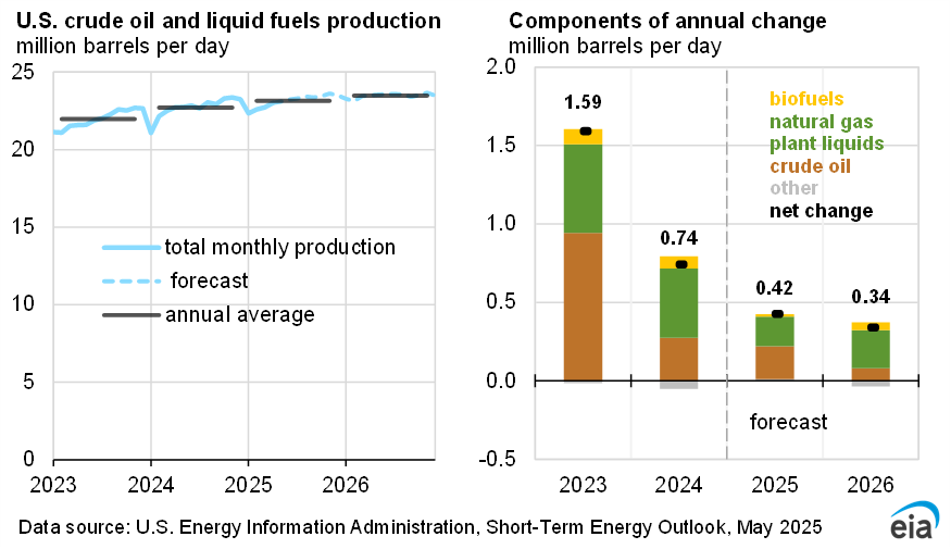This site is protected by reCAPTCHA and the Google Privacy Policy and Terms of Service apply.